Optimal Refund and Ordering Decisions for Fresh Produce E-Commerce Platform: A Comparative Analysis of Refund Policies

Abstract

Different refund policies offered by e-commerce platforms provide diverse options for consumers and are crucial for enhancing after-sales service. This study constructs a refund and ordering decision model based on three typical refund policies: both basic refund and refund guarantee option (‘Policy I’), basic refund only (‘Policy II’), and refund guarantee option only (‘Policy III’). We examine scenarios where demand is influenced by price, refund policies, and stochastic factors, and returns are affected by refund policies, aiming to determine the optimal refund and ordering decisions for fresh produce e-commerce platforms. Our results indicate that, under the same parameters, the platform achieves the maximum order quantity and highest expected profit with Policy I. The return rate under Policy I is always higher than under Policy III, but not consistently higher than under Policy II. Additionally, as the sensitivity of demand to the refund policy increases, both the order quantity and basic refund price rise, while the refund guarantee option price decreases. Conversely, as the sensitivity of returns to the refund policy increases, the opposite occurs. Although market demand uncertainty does not impact the basic refund or refund guarantee option prices, the platform must increase order quantities to manage market volatility.

1. Introduction

Fresh produce generally refers to fresh fruits, vegetables, meat, poultry, eggs, etc., which are closely related to people, and are indispensable components of the human diet [1]. In the past decade, with the improvement of the quality of life and the pursuit of a healthy diet, the demand for fresh produce has been growing steadily. According to the Agrifood Industry 2023 Outlook, the global market for fresh produce is expected to reach about USD 12 trillion by 2027 [2]. With the development of internet technology, e-commerce for fresh produce is experiencing explosive growth. In particular, during the epidemic of COVID-19, due to the need for home isolation and social distancing, online shopping became more popular in life. This popularity has carried over to the shopping behavior of fresh produce, as many consumers are willing to purchase high-quality, fresh produce via e-commerce platforms such as Taobao, Tmall, Jingdong, etc. According to the “2023 China Agricultural Products E-commerce Development Report”, the transaction scales of fresh produce e-commerce reached CNY 560.14 billion in 2022, marking a 20.25% increase compared to 2021. An increasing number of traditional fresh produce producers are partnering with e-commerce platforms to achieve long-term sustainable business development. However, due to the inherent uncertainties of online shopping, particularly for perishable fresh produce, consumers tend to have stringent requirements regarding product freshness. The lack of tactile and sensory evaluation in online purchasing further exacerbates consumer concerns. According to a survey conducted in the United States, approximately 55% of consumers refrain from purchasing fresh produce online due to concerns over freshness [3]. Therefore, effectively enhancing consumer trust and increasing their purchase intention has become a critical issue for fresh produce e-commerce platforms.

In order to provide better service to consumers, e-commerce platforms have introduced return policies to alleviate the impact of this uncertainty [4]. It has been found that by offering flexible return policies, platforms can establish trust with consumers, reduce consumers’ concerns and perceived risks [5], thereby attracting more consumer demand. At the same time, it helps platforms build a good reputation, which is crucial for enhancing platforms competitiveness and sustainable development. Empirical research by Suwelack et al. [6] indicated that the provision of return policies can stimulate consumers’ positive emotional responses, then increasing their willingness to purchase and pay. This allows consumers to shop with confidence and boosts sales demand. Common return policies include unconditional refunds and conditional refunds. For example, if someone is not 100% satisfied with the products they receive, the Fresh Market will refund or replace his/her products, regardless of whether the products are old or new, the purchase period, or whether or not they have been used [7]. Amazon Fresh allows refunds within 30 days if customers are dissatisfied with the product [8]. On Taobao, some merchants, after reviewing return requests and evidence, offer partial refunds for orders with issues such as missing items, defects, or similar problems. While return and refund policies can stimulate demand, they may also increase impulsive purchases and the likelihood of returns [9], impacting retailer profitability [10]. Unconditional full refund policies can lead to fraudulent returns [11], while partial refunds may diminish consumer trust. For perishable and easily damaged fresh produce, overly lenient refund policies can cause significant quality loss, highlighting the need for optimal refund policy research.

Most of the existing studies on fresh produce supply chains have focused on aspects such as product pricing and inventory management [12,13,14,15]. However, there is relatively little research on return and refund policies for fresh produce. Pasternack [16] analyzed optimal pricing and return policies for perishable products using a single-period inventory model, showing that offering partial refunds for unsold goods can achieve channel coordination in multi-retailer environments. Li et al. [17] investigated optimal return and refund policies for perishable goods sold online, analyzing three refund policies (no refund, full refund, and partial refund) and two return requirements (product return and no return). They found that when product returns are required and return costs are high, a more lenient refund policy is preferable. If return costs and rates exceed a threshold, it is optimal not to require product returns. For fresh produce, unconditional full refunds can harm retailer profitability, and conditional partial refunds may impact consumer trust. This paper introduces the refund guarantee option, allowing consumers to obtain an unconditional full refund guarantee through its purchase. We analyze three refund policies to determine the optimal policy: (i) both basic refund and refund guarantee option (Policy I); (ii) only basic refund (Policy II); and (iii) only refund guarantee option (Policy III). Additionally, existing research on return quantity has approached the topic in different ways: some treat the return quantity as a function of a fixed return rate [16,17,18], while some consider the return quantity as an increasing function of the demand and price [19,20]. In reality, the return quantity is more likely influenced by the return policy itself. Referring to the work of Li et al. [21], we model the return quantity as a linear function of baseline returns and the refund policy. Additionally, market demand is influenced by both the refund policy and stochastic factors. Therefore, we examine scenarios where demand is influenced by price, refund policies, and stochastic factors, and returns are affected by refund policies to analyze the optimal refund policy for the e-commerce platform.

This study differs from extant research in three key aspects. First, while previous studies primarily focus on basic refund policies, this paper not only examines basic refund policies but also introduces the refund guarantee option into the analysis of refund policies for fresh produce. Second, in prior research, demand is typically modeled as a function of price, basic refund policies, or consumer utility, while return quantity is often linked to basic refund policies, product quality, or return rates. In contrast, this study assumes that both the demand and return quantity are influenced by price and various refund policies, and we account for the impact of stochastic factors on demand. Lastly, this paper also investigates which refund policy results in the lowest return rate and how changes in various market parameters under the three refund policies affect the platform’s optimal decisions.

Based on these backgrounds, this paper considers how consumer demand and return quantity are affected by refund policies, and constructs the optimal expected revenue model for fresh produce e-commerce platforms. We mainly study the following issues:

(1)

Which refund policy is optimal?

(2)

How do refund policies impact ordering decisions?

(3)

Which refund policy results in the lowest return rate?

(4)

How do changes in various market parameters impact the optimal decisions?

To answer the above questions, we assume that a fresh produce e-commerce platform faces a consumer market of stochastic size. These consumers are uncertain whether the fresh produce will meets their needs and preferences until they receive the products. The e-commerce platform provides a refund policy to enhance service levels. Thus, demand is influenced by price, basic refund price, refund guarantee option price, and stochastic factors. The e-commerce platform orders a certain quantity of fresh produce from a producer, who produces based on the order quantity. The study examines the platform’s optimal refund and ordering decisions under stochastic demand. The specific work is as follows. Firstly, by constructing the demand, return function, and expected revenue model of the e-commerce platform under three refund policies, we solve for the optimal values of each decision variable. Secondly, we compare and analyze the expected revenue and rates of return of the e-commerce platform under the three refund policies. Finally, through numerical simulation, we analyze how each decision variable is affected by the deterioration rate and sensitivity coefficients, as well as how these variables, deterioration rate, and other parameters impact the platform’s expected revenue.

The rest of this paper is sorted out as follows: Section 2 presents the related literature. Section 3 explains the model assumptions and related parameters. Section 4 constructs the models and solves them, providing the equilibrium results under the three refund policies and expressing the optimal decision variables. Section 5 discusses the optimal refund policy of the e-commerce platform and their impact on the profit of the e-commerce platform through numerical simulation under the three refund policies. It also includes the sensitivity and visualization analysis of related parameters. Section 6 summarizes the research and discusses the future research directions.

2. Literature Review

This section reviews the literature on product return policies, as well as ordering and inventory policies for fresh produce.

2.1. Return Policies

A review of the literature reveals that existing research on return policies primarily covers three aspects: (1) the impact of return policies, (2) retailers’ refund methods, and (3) return channels.

Regarding the impact of return policies, extant research is mainly divided into two areas: positive impacts and negative impacts. The positive impacts of return policies are generally considered to include reducing consumer risk, increasing willingness to pay, boosting sales, and enhancing revenue. Che [22] found that return policies not only reduce consumers’ anticipated losses but also enable retailers to set higher prices. Batarfi et al. [23] discovered that a moderately lenient return policy can lower perceived risk, increase purchase intent, and boost sales. Wood [24] showed that return policies can signal quality to consumers, reduce concerns, and encourage spending. Mukhopadhyay and Setoputro [25] examined optimal return policies and modular design for made-to-order products, finding that a lenient return policy and higher modularity can enhance sales revenue. Li et al. [26] divided sales into normal and discount periods, analyzing optimal return, pricing, and ordering strategies. Their results indicated that offering a money-back guarantee (MBG) and reselling returned products are not always advantageous for retailers; both MBG and non-MBG return strategies can potentially benefit retailers and achieve Pareto improvement in the supply chain. Ma et al. [27] studied the impact of virtual showrooms, exchange policies, and full refund return policies on platforms, finding that all three strategies positively affect platform demand, with exchange and full refund policies offering additional benefits.

Although research indicates that consumer return behavior is primarily influenced by product quality [28,29], lenient return policies can also provoke opportunistic behavior [30]. Opportunistic consumers fall into two categories: one group returns products after price reductions to minimize payment costs [31], leading some retailers to offer price adjustment services during sales to deter such behavior. The other group returns products after exploiting their trial value [32], prompting retailers to impose restrictions, such as requiring clothing returns to retain tags and remain unwashed. Khouj et al. [33] explored how opportunistic behavior affects online pricing, ordering quantities, and return policies. They found that retaining products benefits consumers more, while store credit and gift card refunds are more advantageous for online retailers. Chen et al. [11] examined the effect of perceived fairness on return policies in the context of fraudulent returns. They discovered that consumers with a strong sense of fairness prefer stricter return policies to combat fraud and view restrictive return policies as fairer.

The substantial body of literature on retailers’ refund methods includes no refund, partial refunds, and full refunds [21,34,35,36]. Fan et al. [4] compared cash refunds with store credit or gift card (SC/GC) refunds, finding that retailers can attract consumers with cash refunds while limiting return rates. Wang et al. [37] investigated the effects of return rates and bidirectional option contracts on return prices and ordering policies. Their findings indicate that higher return rates lead to lower optimal return prices and reduced order quantities. Firms should not offer refunds at high return rates, provide partial refunds at moderate rates, and offer full refunds when return rates are low.

Existing research on return channels primarily focuses on online and offline aspects. Mandal et al. [38] developed various sales models, including online-only sales, showroom and online sales (i.e., offline experience followed by online purchase), and sales through both online and physical stores with returns handled in physical stores. They found that if return rates are high, retailers should establish showrooms for pre-purchase experiences, while low online return costs favor online-only sales. Gao et al. [39] examined the impact of omnichannel returns on the number and size of physical stores, revealing that higher online return rates lead retailers to open fewer but larger physical stores. Nageswaran et al. [40] studied customer return strategies in omnichannel operations. They found that online stores with numerous return partners and omnichannel retailers with many physical stores should offer full refunds. However, for retailers with many online stores and physical stores that can effectively retain customers, charging fees for online returns can incentivize customers to visit physical stores.

This study does not address return channels. We focus on designing refund policies to maximize benefits while minimizing opportunistic returns. Therefore, we introduce refund guarantee options into the refund policies for fresh produce and examine optimal decision-making under three refund policies.

2.2. The Ordering and Inventory Strategies for Fresh Produce

The extant literature on ordering and inventory strategies for fresh produce primarily explores the impact of deterministic and uncertain demand on decision-making.

Regarding ordering and inventory decisions for fresh produce under deterministic demand, Qin et al. [41] investigated joint pricing and inventory control incorporating quality and quantity losses. Their results show that when demand price sensitivity is low, sellers can increase profits by raising prices, increasing reorder quantities, and shortening replenishment cycles. When quality degradation rates are low, sellers can enhance profits by extending reorder times and increasing order quantities. He et al. [42] studied pricing and ordering decisions for fresh produce based on quality grading. Fan et al. [43] developed a dynamic pricing and replenishment model considering consumer choice behavior, finding that order quantities depend on both the freshness and inventory of the remaining produce when the inventory falls below a threshold, and only on freshness when above the threshold. Pando et al. [44] examined an inventory model based on inventory costs and demand rates, revealing that optimal order quantities are directly proportional to the replenishment costs and inversely proportional to the unit purchase prices. Wu et al. [45] considered demand as a multivariate function of freshness, shelf quantity, and shelf life to study optimal reorder cycles and end-of-period inventory levels. Feng et al. [46] proposed an inventory model where the deterministic demand for perishable goods is a multivariate function of price, freshness, and display inventory, studying optimal reorder times, sales prices, and end-of-period inventory levels.

Due to market uncertainty, many scholars have also studied ordering and inventory decisions under stochastic demand. Muriana [47] examined a stochastic inventory model for perishable goods with normally distributed demand. Minner and Transchel [48] explored how demand and order variability are influenced by product perishability and proposed a dynamic ordering strategy for the upstream supply stage, considering negative correlation between orders. Wang and Chen [49] investigated ordering and pricing decisions for fresh produce under stochastic demand, incorporating put options and product transportation losses, finding that optimal order quantities and sale prices decrease with lower option prices but increase with higher exercise prices and distribution losses. Dolat-Abad [50] developed a two-part tariff contract coordination strategy to reduce product waste and studied the optimal retail prices, order quantities, promotional efforts, and wholesale prices for fresh produce retailers, finding that coordination increases order quantities and promotional efforts while reducing prices and waste.

This study addresses both the impact of stochastic factors on ordering decisions for fresh produce and the influence of various refund policies on optimal ordering decisions. Our main contributions are threefold: First, we introduce the refund guarantee option into the refund policies for fresh produce and investigate optimal decisions under three refund policies. Second, we examine the effects of refund policies on ordering decisions. Finally, we compare return rates across three refund policies and analyze how changes in market parameters affect optimal decisions, providing insights for the management of fresh produce e-commerce platforms.

3. Notations and Assumptions

3.1. Notations

The following notations in

Table 1. Notations description.

Decision Variables	Description
r	Basic refund price $\left(\begin{array}{c}0\le r\le p\end{array}\right)$
o	Refund guarantee option price $\left(\begin{array}{c}0\le o\le p\end{array}\right)$
q	Order quantity
Model parameters	Description
c	The unit cost of fresh produce (including procurement, transportation, storage, and preservation expenses)
p	Selling price of fresh produce
$\theta (\theta \in [0,1\left)\right)$	Deterioration rate of fresh produce
$\nu$	The unit residual value of returned fresh produce after deducting the shipping fee $(\nu <p)$
k	The unit residual value of remaining fresh produce ($k<p$)
$T_i(i=1,2,3)$	Return rate for Policy i
$D_{i1}(i=1,2,3)$	The sum of the basic market demand and the price-affected market demand
$D_{i2}(i=1,2,3)$	Market demand affected by the basic refund policy
$D_{i3}(i=1,2,3)$	Market demand affected by the refund guarantee option policy $(\nu <p)$
$D_1$	The demand function when the e-commerce platform offers both basic refund and refund guarantee option policies.
$D_2$	The demand function when the e-commerce platform offers the basic refund policy
$D_3$	The demand function when the e-commerce platform offers the refund guarantee option policy
$R_{i1}(i=1,2,3)$	Market’s basic return quantity
$R_{i2}(i=1,2,3)$	Return quantity affected by the basic refund policy
$R_{i3}(i=1,2,3)$	Return quantity affected by the refund guarantee option policy
$R_1$	The return function when the e-commerce platform offers both basic return and refund guarantee option policies
$R_2$	The return function when the e-commerce platform offers the basic refund policy
$R_3$	The return function when the e-commerce platform offers the refund guarantee option policy
${\Pi }_1$	Profit objective function of the e-commerce platform when offering both basic refund and refund guarantee option policies
${\Pi }_2$	Profit objective function of the e-commerce platform when offering the basic refund policy
${\Pi }_3$	Profit objective function of the e-commerce platform when offering the refund guarantee option policy

$i=1,2,3$ represent Policies I, II, III, respectively.

have been used in model formulation.

3.2. Assumptions

(i)

Assumption 1: The product’s deterioration rate remains constant over time and does not reach complete deterioration, i.e., the rate is less than 1. Following Min et al. [51], who used $0<\theta <1$ to avoid extreme cases, we adopt a similar assumption but also consider the case where the deterioration rate is zero, i.e., $0\le \theta <1$.

(ii)

Assumption 2: After consumers submit return requests on the platform and send the products back, the platform determines the refund method based on whether the consumers purchased the option. Since the platform needs to determine the refund method based on the quantity of returned products and whether the consumer purchased an option, the refund must be processed after receiving the goods.

(iii)

Assumption 3: Restocking is not allowed, and inventory costs and stock out penalty costs are not considered. This simplifies the model, allowing the research to focus more on the impact of the refund policies without being affected by inventory and restocking issues.

(iv)

Assumption 4: The platform covers the shipping cost for returns, which boosts consumer trust and purchase willingness, while the unit residual value is the value after deducting the shipping cost.

(v)

Assumption 5: The residual value of spoiled products is ignored, and no additional costs are incurred. This simplifies the model, as the salvage value of deteriorated fresh produce is significantly reduced.

(vi)

Assumption 6: The unit residual value of surplus and returned fresh produce is assumed to be lower than the unit wholesale cost ($k<c$, $\nu <c$), which helps the platform avoid excessive product accumulation and encourages quality and service improvements, reducing return rates.

(vii)

Assumption 7: Due to the increased risk of damage and the reduced residual value of returned products after deducting shipping costs, we assume that the residual value of returned products does not exceed that of the surplus, i.e., $\nu \le k$

4. Model Construction and Solution Analysis

4.1. Problem Description

In this article, considering that the demand is affected by price, basic refund price, refund guarantee option price, and stochastic factors, while returns are affected by basic refund price and refund guarantee option price, we study three typical refund policies—both basic refund and refund guarantee option policies (‘Policy I’), basic refund policy (‘Policy II’), refund guarantee option policy (‘Policy III’)—and construct the refund and ordering decisions model to investigate the optimal refund and order decisions for the e-commerce platform of fresh produce. Specifically, before the start of the sales season, the platform pre-orders a certain quantity of products from fresh produce producers. The producers operate on a make-to-order basis and sell them to the e-commerce platform at a predetermined wholesale price when the sales season begins. The platform determines the selling price by combining the wholesale price and market price. This price is predetermined and serves as a model parameter rather than a decision variable, as the price of fresh produce is often significantly influenced by market competition. Additionally, refund policies are provided during the sales process. If consumers are dissatisfied with the received fresh produce, they can request a refund from the platform. This article investigates the refund and ordering decisions that maximize the platform’s expected revenue.

4.1.1. Sales Methods

This article considers an e-commerce platform for fresh produce ordering a certain quantity of fresh produce from a supplier and selling them online. The specific sales process is as follows: First, the platform determines the selling price p based on the wholesale price and market price (assuming p is fixed in a perfectly competitive market). Then, consumers purchase the products at the price on the platform and choose whether to purchase the refund guarantee option or not. Subsequently, after receiving the products, consumers decide whether to return them considering the product’s characteristics, their expectations regarding the product, and the platform’s refund policy. Finally, if consumers request a return, refunds are processed according to the following two methods: (1) Assuming consumers have not purchased the refund guarantee option, after applying for a return, they return the product to the platform. Meanwhile, the platform returns a certain basic refund price r$\left(\begin{array}{c}0\le r\le p\end{array}\right)$ to the consumer (basic refund policy), where $(p-r)$ represents the refund fee charged by the platform to the consumer. When $r=0$, it indicates no refund, and when $r=p$, it signifies a full refund. A higher r implies a better refund policy to the consumer. (2) Assuming consumers have purchased the option o$\left(\begin{array}{c}0\le o\le p\end{array}\right)$, after applying for a return, consumers return the product to the platform. The platform then refunds the selling price p to the consumer (Refund guarantee option policy). Here, o represents the fee charged by the platform to the consumer. (Assuming that a portion of the produce is consumed, then, if the consumer has purchased the option, the remaining product is refunded at the original price; otherwise, it is refunded at the basic refund price.) It is important to note that we assume $r\le (p-o)$ in Policy I; only under this condition would consumers consider purchasing with the refund guarantee option.

4.1.2. Demand Functions

In line with the research objective of this article, we assume that the better the refund policy offered by an e-commerce platform, the more market demand it can attract. Conversely, we hypothesize that insufficiently friendly refund policies provided by e-commerce platforms may result in a decrease in demand.

(1) This article assumes that market demand is subject to uncertainty. Without loss of generality, we assume that the demand function is linear, which has been widely used in previous research [52,53]. When not considering the impact of refund guarantee option and basic refund policies on demand, the basic demand function takes the following form:

$$D_{i1}=a-bp+\epsilon (i=1,2,3)$$

(1)

where $\epsilon$ is a stochastic parameter, whose cumulative distribution function and probability density function are denoted as $F(·)$ and $f(·)$, respectively. We assume that the probability density function $f(·)$ is symmetric about the y-axis on the interval $[-A,A],A>0$. $a(a>0)$ represents the fundamental demand, which is unaffected by prices and refund factors but only influenced by non-price factors such as inherent consumer preferences. $b(b>0)$ represents the sensitivity coefficient of market demand to prices. $i=1,2,3$ denote Policies I, II, and III, respectively, hereinafter.

(2) If the consumer does not purchase the option, we assume that the market demand attracted by the basic return price is denoted as

$$D_{i2}=w_{1}r(i=1,2,3)$$

(2)

where r represents the basic refund price, and $w_1(w_1>0)$ represents the sensitivity coefficient of market demand to the basic refund policy. (3) If the consumer purchases the refund guarantee option o, the platform can provide a full refund of the selling price p. Considering that the consumer has paid an additional option price o when purchasing the product, the effective payment price from the platform to the consumer is therefore $(p-o)$. Assuming that the market demand is attracted by the refund guarantee option is represented as

$$D_{i3}=w_2(p-o)(i=1,2,3)$$

(3)

where $w_2(w_2>0)$ is the sensitivity factor of the market demand to the refund guarantee option price.

4.1.3. Return Functions

Consumers weigh the pros and cons of the platform’s refund policies to decide whether to purchase a refund guarantee option and whether to return the product. If the received product does not meet expectations and the platform’s refund policy is better, consumers will be more inclined to return the product, leading to an increase in return quantity. The model uses the return function formula from Li et al. [21].

(1) Regardless of the refund policy adopted by the platform, there exists basic return quantity $\phi (\phi >0)$ in the market that is not affected by the refund factors, denoted as

$$R_{i1}=\phi (i=1,2,3)$$

(4)

(2) The market return quantity is attracted by the basic refund policy, denoted as

$$R_{i2}=u_{1}r(i=1,2,3)$$

(5)

where $u_1(u_1>0)$ is the sensitivity coefficient of the return quantity to the basic refund policy.

(3) The amount of market returns is attracted by the refund guarantee option policy, denoted as

$$R_{i3}=u_2(p-o)(i=1,2,3)$$

(6)

where $u_2(u_2>0)$ is the sensitivity coefficient of the return quantity to the refund guarantee option policy.

Based on the basic properties of the sensitivity coefficients in the market, there are some relationships between these coefficients. Consumers are more sensitive to price than to the basic refund and refund guarantee option policies, i.e., $b>w_1$ and $b>w_2$. This reflects the realistic priority consumers place on price over refund conditions. Additionally, since consumers bear extra costs for the refund guarantee option, it stimulates demand less effectively than the basic refund policy. Thus, the sensitivity to the basic refund policy is not less than that of the refund guarantee option, i.e., $w_1\ge w_2$. At the same time, the consumer demand attracted by the platform’s refund policies is not less than the corresponding return quantity, i.e., $w_1\ge u_1$ and $w_2\ge u_2$. This reflects the platform’s incentive to offer refund policies only when demand sensitivity exceeds return sensitivity. Furthermore, the basic market demand is not less than the basic return quantity, i.e., $a\ge \phi$, ensuring the platform maintains profitability by avoiding excessive returns.

4.2. Model

There are three kinds of refund policies for the e-commerce platform: Policy I offers both basic refund and refund guarantee option policies; Policy II offers the basic refund policy; Policy III: offers only the refund guarantee option policy. Below, we will construct and analyze the model for an e-commerce platform using three refund policies.

4.2.1. Offering Both Basic Refund Policy and Refund Guarantee Option Policy

Based on the aforementioned formulas, the market demand function for the e-commerce platform under Policy I is

$$D_1=D_{11}+D_{12}+D_{13}=a-bp+w_{1}r+w_2(p-o)+\epsilon$$

(7)

The market return quantity function is

$$R_1=R_{11}+R_{12}+R_{13}=\phi +u_{1}r+u_2(p-o)$$

(8)

Given the wholesale price c, the e-commerce platform needs to choose the optimal order quantity q, the basic refund price r and the refund guarantee option price o to maximize the expected revenue, and the platform’s profit function is

$$\begin{array}{cc}\hfill {\Pi }_1& =\underset{q,r,o}{max}(p·E[min(q(1-\theta ),D_1)]+D_{13}o-(R_{11}+R_{12})r-R_{13}p\hfill \\ & +(R_{11}+R_{12}+R_{13})v+k{[q(1-\theta )-D_1]}^{+}-qc)\hfill \end{array}$$

(9)

Referring to Petruzzi and Dada [54], when demand exceeds $q(1-\theta )$, the e-commerce platform’s profit is $pq(1-\theta )$, and when demand is lower than $q(1-\theta )$, the platform’s profit is $p{D}_1$. To simplify the notation, let $G_1=D_{13}o-(R_{11}+R_{12})r-R_{13}p+(R_{11}+R_{12}+R_{13})\nu -qc$ and $z_1=q(1-\theta )-(a-bp+w_{1}r+w_2(p-o))$, Then, the profit objective function of the e-commerce platform can be formulated as

$$\begin{array}{c}\hfill {\Pi }_1=\left\{\begin{array}{cc}p(1-\theta )q+G_1\hfill & A\ge \epsilon >z_1\hfill \\ p{D}_1+G_1+k{[q(1-\theta )-D_1]}^{+}\hfill & -A\le \epsilon \le z_1\hfill \end{array}\right.\end{array}$$

(10)

where $z_1=(q(1-\theta )-(a-bp+w_{1}r+w_2(p-o)))\in \left[-\mathrm{A},\mathrm{A}\right]$, $r\le (p-o)$. In $G_1$, the first term represents the additional revenue to the platform from consumers purchasing the option. The second term represents the total refund amount for returns from consumers without the option, while the third term covers refunds for those with the option. The fourth term is the total residual value of the returned products. The fifth term is the total wholesale cost.

In Equation (10), when the quantity of unspoiled inventory is below the demand, the platform’s revenue is $p(1-\theta )q$. Otherwise, the platform’s revenue is $p{D}_1$. $k{[q(1-\theta )-D_1]}^{+}$ represents the total residual value of the remaining products.

Theorem 1.

When the e-commerce platform adopts Policy I, its expected revenue function is concave and has a unique optimal value.

Proof of Theorem 1.

From Equation (9), the objective of the platform is to maximize the expected revenue function $E\left({\Pi }_1(q,r,o)\right)$ within three constraint conditions. The problem can be represented using the following equation:

$$\begin{array}{cc}\hfill & max\left[E\left({\Pi }_1(q,r,o)\right)\right]=max\left[(p-k){\int }_{-A}^{z_1}\left[(a-bp+w_{1}r+w_2(p-o)+u)\right]f\left(u\right)du\right.\hfill \\ \hfill & +(k-p)(1-\theta )q{\int }_{-A}^{z_1}f\left(u\right)du+(1-\theta )pq+w_2(p-o)o\hfill \\ \hfill & \left.-(\phi +u_{1}r)r-u_2(p-o)p+[\phi +u_{1}r+u_2(p-o)]\nu -qc\right]\hfill \\ \hfill & \mathrm{subject}\mathrm{to}\left\{\begin{array}{cc}p-o-r\ge 0\hfill & (\mathrm{Constraint}1)\hfill \\ A-z_1\ge 0\hfill & (\mathrm{Constraint}2)\hfill \\ A+z_1\ge 0\hfill & (\mathrm{Constraint}3)\hfill \end{array}\right.\hfill \end{array}$$

(11)

Taking the first-order partial derivative of the expected revenue function, $E\left({\Pi }_1(q,r,o)\right)$, yields

$${\displaystyle \frac{\partial E\left({\Pi }_1(q,r,o)\right)}{\partial q}}=(k-p)(1-\theta )F\left(z_1\right)+(1-\theta )p-c$$

(12)

$${\displaystyle \frac{\partial E\left({\Pi }_1(q,r,o)\right)}{\partial r}}=(p-k)w_{1}F\left(z_1\right)-\phi -2u_{1}r+u_1\nu$$

(13)

$${\displaystyle \frac{\partial E\left({\Pi }_1(q,r,o)\right)}{\partial o}}=(k-p)w_{2}F\left(z_1\right)+w_{2}p-2w_{2}o+u_{2}p-u_{2}v$$

(14)

The Hessian matrix of $E\left({\Pi }_1(q,r,o)\right)$ is

$$\left[\begin{array}{ccc}(k-p){(1-\theta )}^{2}f\left(z_1\right)& (p-k)(1-\theta )w_{1}f\left(z_1\right)& (k-p)(1-\theta )w_{2}f\left(z_1\right)\\ (p-k)(1-\theta )w_{1}f\left(z_1\right)& (k-p)w_1^{2}f\left(z_1\right)-2u_1& (p-k)w_1{w}_{2}f\left(z_1\right)\\ (k-p)(1-\theta )w_{2}f\left(z_1\right)& (p-k)w_1{w}_{2}f\left(z_1\right)& (k-p)w_2^{2}f\left(z_1\right)-2w_2\end{array}\right]$$

(15)

Therefore, the Hessian matrix is negative definite, indicating that the original objective function is concave. Furthermore, since all constraints of the original problem are convex functions, the problem can be transformed into a convex optimization problem, i.e., minimizing $-E\left({\Pi }_1(q,r,o)\right)$ under the same constraints. Then, by utilizing the Karush–Kuhn–Tucker (KKT) conditions to solve the minimization problem for the optimal solution, substituting them into the original objective function yields the maximum value of the expected revenue function:

$$\begin{array}{cc}\hfill & \min (k-p){\int }_{-A}^{z_1}\left[(a-bp+w_{1}r+w_2(p-o)+u)\right]f\left(u\right)du+(p-k)(1-\theta )q{\int }_{-A}^{z_1}f\left(u\right)du\hfill \\ \hfill & -(1-\theta )pq-w_2(p-o)o+(\phi +u_{1}r)r+u_2(p-o)p-[\phi +u_{1}r+u_2(p-o)]\nu +qc\hfill \\ \hfill & \mathrm{subject}\mathrm{to}\left\{\begin{array}{cc}p-o-r\ge 0\hfill & (\mathrm{Constraint}1)\hfill \\ A-z_1\ge 0\hfill & (\mathrm{Constraint}2)\hfill \\ A+z_1\ge 0\hfill & (\mathrm{Constraint}3)\hfill \end{array}\right.\hfill \end{array}$$

(16)

The KKT conditions for the convex optimization problem (16) are shown in Equations (17)–(28):

$$(p-k)(1-\theta )F\left(z_1\right)-(1-\theta )p+c+{\lambda }_2(1-\theta )-{\lambda }_3(1-\theta )=0$$

(17)

$$(k-p)w_{1}F\left(z_1\right)+\phi +2u_{1}r-u_1\nu +{\lambda }_1-{\lambda }_2{w}_1+{\lambda }_3{w}_1=0$$

(18)

$$(p-k)w_{2}F\left(z_1\right)-w_{2}p+2w_{2}o-u_{2}p+u_{2}v+{\lambda }_1+{\lambda }_2{w}_2-{\lambda }_3{w}_2=0$$

(19)

$${\lambda }_1(p-o-r)=0$$

(20)

$${\lambda }_2(A-z_1)=0$$

(21)

$${\lambda }_3(A+z_1)=0$$

(22)

$$p-o-r\ge 0$$

(23)

$$A-z_1\ge 0$$

(24)

$$A+z_1\ge 0$$

(25)

$${\lambda }_1\ge 0$$

(26)

$${\lambda }_2\ge 0$$

(27)

$${\lambda }_3\ge 0$$

(28)

Since A > 0, it implies that ${\lambda }_2$ and ${\lambda }_3$ cannot both take non-zero values, as otherwise, we would have $A-z_1=A+z_1=0\Rightarrow A=0$ and $z_1=0$, which contradicts the fact that A > 0. Therefore, we discuss the following six cases to solve Equation (16):

$$\begin{array}{cc}& \mathrm{Case}{I}^1:{\lambda }_2=0,{\lambda }_3=0,{\lambda }_1=0;\mathrm{Case}{I}^2:{\lambda }_2=0,{\lambda }_3=0,{\lambda }_1\ne 0;\hfill \\ & \mathrm{Case}{I}^3:{\lambda }_2=0,{\lambda }_3\ne 0,{\lambda }_1=0;\mathrm{Case}{I}^4:{\lambda }_2=0,{\lambda }_3\ne 0,{\lambda }_1\ne 0;\hfill \\ & \mathrm{Case}{I}^5:{\lambda }_3=0,{\lambda }_2\ne 0,{\lambda }_1=0;\mathrm{Case}{I}^6:{\lambda }_3=0,{\lambda }_2\ne 0,{\lambda }_1\ne 0.\hfill \end{array}$$

This minimization problem is a convex optimization problem, whose KKT points, local minima, and global minima are equivalent. Due to the lack of specific parameter values, we can only determine all possible KKT points, that is, all possible values of the optimal solution. Below, we discuss the analytical expressions of the KKT points corresponding to six different scenarios, addressing the optimal solutions for each of these six cases.

• $\mathrm{Case}{I}^1:{\lambda }_2=0,{\lambda }_3=0,{\lambda }_1=0$

In this case, none of the three constraints are effective. When $p-r^{*}-o^{*}=w_2\phi +u_1{w}_2(2p-\nu -{\displaystyle \frac{c}{1-\theta }})-w_1{w}_2(p-{\displaystyle \frac{c}{1-\theta }})-u_1{u}_2(p-\nu )\ge 0$, the first constraint is satisfied. When $k-{\displaystyle \frac{c}{1-\theta }}\le 0$, the second constraint is satisfied. When ${\displaystyle \frac{c}{1-\theta }}-p\le 0$, the third constraint is satisfied. If all the three constraints are satisfied, we obtain the analytical expression of the optimal solution as follows:

$$r^{*}={\displaystyle \frac{w_{1}p+u_1\nu -\phi -\frac{c}{1-\theta }{w}_1}{2u_1}}$$

(29)

$$o^{*}={\displaystyle \frac{u_2(p-\nu )+\frac{c}{1-\theta }{w}_2}{2w_2}}$$

(30)

$$q^{*}={\displaystyle \frac{F^{-1}\left(\frac{c-(1-\theta )p}{(p-k)(1-\theta )}\right)+(a-bp+w_1{r}^{*}+w_2(p-o^{*}))}{1-\theta }}.$$

(31)

Since all constraints are inactive, the maximum point of the original problem can be attained:

• $\mathrm{Case}{I}^2:{\lambda }_2=0,{\lambda }_3=0,{\lambda }_1\ne 0$

In this case, only the first constraint is effective. When $k-{\displaystyle \frac{c}{1-\theta }}\le 0$ and ${\displaystyle \frac{c}{1-\theta }}-p\le 0$ are satisfied, the second and third constraints are respectively satisfied. If ${\lambda }_1=(p-k)w_{1}F(q^{*}(1-\theta )-(a-bp+w_1{r}^{*}+w_2(p-o^{*}))-\phi -2u_1{r}^{*}+u_1\nu >0$, we obtain the analytical expression of the optimal solution as follows:

$${\lambda }_1=(p-k)w_{1}F(q^{*}(1-\theta )-(a-bp+w_1{r}^{*}+w_2(p-o^{*})))-\phi -2u_1{r}^{*}+u_{1}v$$

(32)

$$r^{*}={\displaystyle \frac{w_{1}p+2w_{2}p-\phi +u_1\nu -u_2(p-\nu )-\frac{c}{1-\theta }(w_1+w_2)}{2(u_1+w_2)}}$$

(33)

$$o^{*}={\displaystyle \frac{2u_{1}p-w_{1}p+\phi -u_1\nu +u_2(p-\nu )+\frac{c}{1-\theta }(w_1+w_2)}{2(u_1+w_2)}}$$

(34)

$$q^{*}={\displaystyle \frac{F^{-1}\left(\frac{c-(1-\theta )p}{(p-k)(1-\theta )}\right)+(a-bp+w_1{r}^{*}+w_2(p-o^{*}))}{1-\theta }}.$$

(35)

• $\mathrm{Case}{I}^3:{\lambda }_2=0,{\lambda }_3\ne 0,{\lambda }_1=0$

In this scenario, only the third constraint is effective. When $p-r^{*}-o^{*}=w_2\phi +u_1{w}_2(2p-\nu -{\displaystyle \frac{c}{1-\theta }})-w_1{w}_2(p-{\displaystyle \frac{c}{1-\theta }})-u_1{u}_2(p-\nu )\ge 0$ and ${\lambda }_3={\displaystyle \frac{c}{1-\theta }}-p>0$, the analytical expression of the optimal solution is given by

$${\lambda }_3={\displaystyle \frac{c}{1-\theta }}-p$$

(36)

$$r^{*}={\displaystyle \frac{w_{1}p+u_1\nu -\phi -\frac{c}{1-\theta }{w}_1}{2u_1}}$$

(37)

$$o^{*}={\displaystyle \frac{u_2(p-\nu )+\frac{c}{1-\theta }{w}_2}{2w_2}}$$

(38)

$$q^{*}={\displaystyle \frac{-A+(a-bp+w_1{r}^{*}+w_2(p-o^{*}))}{(1-\theta )}}.$$

(39)

• $\mathrm{Case}{I}^4:{\lambda }_2=0,{\lambda }_3\ne 0,{\lambda }_1\ne 0$

In this scenario, the second and third constraints come into play, so the analytical expression for the optimal solution is obtained when ${\lambda }_1=w_{1}p-\phi -2u_1{r}^{*}+u_1\nu -{\displaystyle \frac{c}{1-\theta }}{w}_1>0$ and ${\lambda }_3={\displaystyle \frac{c}{1-\theta }}-p>0$:

$${\lambda }_1=w_{1}p-\phi -2u_1{r}^{*}+u_1\nu -{\displaystyle \frac{c}{1-\theta }}{w}_1$$

(40)

$${\lambda }_3={\displaystyle \frac{c}{1-\theta }}-p$$

(41)

$$r^{*}={\displaystyle \frac{w_{1}p+2w_{2}p-\phi +u_1\nu -u_2(p-\nu )-\frac{c}{1-\theta }(w_1+w_2)}{2(u_1+w_2)}}$$

(42)

$$o^{*}={\displaystyle \frac{2u_{1}p-w_{1}p+\phi -u_1\nu +u_2(p-\nu )+\frac{c}{1-\theta }(w_1+w_2)}{2(u_1+w_2)}}$$

(43)

$$q^{*}={\displaystyle \frac{-A+(a-bp+w_1{r}^{*}+w_2(p-o^{*}))}{(1-\theta )}}.$$

(44)

• $\mathrm{Case}{I}^5:{\lambda }_3=0,{\lambda }_2\ne 0,{\lambda }_1=0$

In this case, only the second constraint is active, and the analytical expression for the optimal solution is obtained by solving $p-r^{*}-o^{*}=w_2\phi +u_1{w}_2(2p-\nu -{\displaystyle \frac{c}{1-\theta }})-w_1{w}_2(p-{\displaystyle \frac{c}{1-\theta }})-u_1{u}_2(p-\nu )\ge 0$ and ${\lambda }_2=k-{\displaystyle \frac{c}{1-\theta }}>0$:

$${\lambda }_2=k-{\displaystyle \frac{c}{1-\theta }}$$

(45)

$$r^{*}={\displaystyle \frac{w_{1}p+u_1\nu -\phi -\frac{c}{1-\theta }{w}_1}{2u_1}}$$

(46)

$$o^{*}={\displaystyle \frac{u_2(p-\nu )+\frac{c}{1-\theta }{w}_2}{2w_2}}$$

(47)

$$q^{*}={\displaystyle \frac{A+(a-bp+w_1{r}^{*}+w_2(p-o^{*}))}{(1-\theta )}}.$$

(48)

• $\mathrm{Case}{I}^6:{\lambda }_3=0,{\lambda }_2\ne 0,{\lambda }_1\ne 0$

In this scenario, only the second constraint is active. When ${\lambda }_1=(p-k)w_1-\phi -2u_1{r}^{*}+u_1\nu +(k-{\displaystyle \frac{c}{1-\theta }})w_1>0$ and ${\lambda }_2=k-{\displaystyle \frac{c}{1-\theta }}>0$, we obtain the analytical expression of the optimal solution as follows:

$${\lambda }_1=(p-k)w_1-\phi -2u_1{r}^{*}+u_1\nu +(k-{\displaystyle \frac{c}{1-\theta }})w_1$$

(49)

$${\lambda }_2=k-{\displaystyle \frac{c}{1-\theta }}$$

(50)

$$r^{*}={\displaystyle \frac{w_{1}p+2w_{2}p-\phi +u_1\nu -u_2(p-\nu )-\frac{c}{1-\theta }(w_1+w_2)}{2(u_1+w_2)}}$$

(51)

$$o^{*}={\displaystyle \frac{2u_{1}p-w_{1}p+\phi -u_1\nu +u_2(p-\nu )+\frac{c}{1-\theta }(w_1+w_2)}{2(u_1+w_2)}}$$

(52)

$$q^{*}={\displaystyle \frac{A+(a-bp+w_1{r}^{*}+w_2(p-o^{*}))}{(1-\theta )}}$$

(53)

Through comparative analysis of the six scenarios mentioned above, we find that $r^{*}$ and $o^{*}$ are influenced solely by the first constraint, while $q^{*}$ is jointly affected by the second and third constraints. Since this problem is a convex optimization problem with a unique KKT point, by substituting specific parameter values to find the KKT point, this point represents the optimal solution to the original problem. Substituting this point back into the objective function of the original problem allows us to obtain the maximum expected revenue when the platform adopts Policy I. □

4.2.2. Basic Refund Policy

When the e-commerce platform adopts Policy II, the market demand function is

$$D_2=D_{21}+D_{22}=a-bp+w_{1}r+\epsilon$$

(54)

The market return function is:

$$R_2=R_{21}+R_{22}=\phi +u_{1}r$$

(55)

At this point, the e-commerce platform has to choose the optimal and to maximize the expected revenue, and the profit function is

$${\Pi }_2=\underset{q,r}{max}p·E[min(q(1-\theta ),D_2)]-(R_{21}+R_{22})r+(R_{21}+R_{22})\nu +k{[q(1-\theta )-D_2]}^{+}-qc$$

(56)

To simplify the notation, let $G_2=-(R_{21}+R_{22})r+(R_{21}+R_{22})\nu -qc$ and $z_2=q(1-\theta )-(a-bp+w_{1}r)$. Then, the profit objective function of the e-commerce platform can be formulated as

$${\Pi }_2=\left\{\begin{array}{cc}p(1-\theta )+G_2\hfill & A\ge \epsilon >z_2\hfill \\ p{D}_2+G_2+k{[q(1-\theta )-D_2]}^{+}\hfill & -A\le \epsilon \le z_2\hfill \end{array}\right.$$

(57)

where $z_2=q(1-\theta )-(a-bp+w_{1}r)\in [-A,A]$. Furthermore, it can be concluded that the platform’s objective is to maximize the expected revenue function $E\left({\Pi }_2(q,r)\right)$ under the two constraints:

$$\begin{array}{cc}\hfill & max\left[E\left({\Pi }_2(q,r)\right)\right]=max\left[(p-k){\int }_{-A}^{z_2}\left[(a-bp+w_{1}r+u)\right]f\left(u\right)du\right.\hfill \\ \hfill & +(k-p)(1-\theta )q{\int }_{-A}^{z_2}f\left(u\right)du+(1-\theta )pq+(\phi +u_{1}r)(\nu -r)-qc]\hfill \\ \hfill & \mathrm{subject}\mathrm{to}\left\{\begin{array}{cc}A-z_2\ge 0\hfill & (\mathrm{Constraint}1)\hfill \\ A+z_2\ge 0\hfill & (\mathrm{Constraint}2)\hfill \end{array}\right.\hfill \end{array}$$

(58)

Theorem 2.

When the e-commerce platform adopts Policy II, its expected revenue function is concave and has a unique optimal value.

4.2.3. Refund Guarantee Option Policy

Assuming that the e-commerce platform adopts Policy III, which only allows returns and refunds for those who have purchased the refund guarantee option, the market demand function is

$$D_3=D_{31}+D_{32}=a-bp+w_2(p-o)+\epsilon$$

(59)

The market return function is

$$R_3=R_{33}=u_2(p-o)$$

(60)

The e-commerce platform has to choose the optimal q and o to maximize the expected revenue, and the profit function of the platform

$${\Pi }_3=\underset{q,o}{max}p·E[min(q(1-\theta ),D_3)]+D_{33}o-R_{3}p+R_3\nu +k{[q(1-\theta )-D_3]}^{+}-qc$$

(61)

To simplify the notation, let $G_3=D_{33}o-R_{3}p+R_3\nu -qc$ and $z_3=q(1-\theta )-(a-bp+w_2(p-o))$. Then, the profit objective function of the e-commerce platform can be formulated as

$${\Pi }_3=\left\{\begin{array}{cc}p(1-\theta )q+G_3\hfill & A\ge \epsilon >z_3\hfill \\ p{D}_3+G_3+k{[q(1-\theta )-D_3]}^{+}\hfill & -A\le \epsilon \le z_3\hfill \end{array}\right.$$

(62)

where $z_3=q(1-\theta )-(a-bp+w_2(p-o))\in [-A,A]$. Furthermore, it can be concluded that the platform’s objective is to maximize the expected revenue function $E\left({\Pi }_3(q,o)\right)$ under the two constraints

$$\begin{array}{cc}\hfill & maxE\left({\Pi }_3(q,o)\right)=max(p-k){\int }_{-A}^{z_3}\left[(a-bp+w_2(p-o)+u)\right]f\left(u\right)du\hfill \\ \hfill & +(k-p)(1-\theta )qF\left(z_3\right)+(1-\theta )pq+w_2(p-o)o+(\nu -p)u_2(p-o)-qc\hfill \\ \hfill & \mathrm{subject}\mathrm{to}\left\{\begin{array}{cc}A-z_3\ge 0\hfill & (\mathrm{Constraint}1)\hfill \\ A+z_3\ge 0\hfill & (\mathrm{Constraint}2)\hfill \end{array}\right.\hfill \end{array}$$

(63)

Theorem 3.

When the e-commerce platform adopts Policy III, its expected revenue function is concave and has a unique optimal value.

The proofs of Theorems 2 and 3 reference the proof of Theorem 1. We discuss the optimal solutions under three different scenarios, and the detailed proof process can be found in Appendix A.

The practical significance of the three theorems is clear. Fresh produce e-commerce platforms can use market-related parameters to verify applicable scenarios. This allows them to make optimal refund and ordering decisions.

4.3. Sensitivity Analysis

Corollary 1.

Under the three refund policies, the expected revenue of the e-commerce platform is positively correlated with the sensitivity coefficient of demand to the refund policy. When $r>\nu >0$, then the expected revenue is negatively correlated with the sensitivity coefficient of returns to the refund policy.

Corollary 1 demonstrates that under the three refund policies, the larger the sensitivity coefficient of consumer demand to the refund policy, the higher the expected revenue of the e-commerce platform. When the basic refund price is higher than the residual value of the returned product, the larger the sensitivity coefficient of consumer returns to refund policies, and the lower the expected revenue of the platform. It is evident that the demand and return quantity to refund policies sensitivity coefficients significantly affect the platform’s revenue, so the platform can effectively improve the expected revenue by improving the consumer demand sensitivity coefficient and reducing the return sensitivity coefficient.

Corollary 2.

Under the three refund policies, the e-commerce platform’s expected revenue decreases as the deterioration rate increases.

Corollary 2 indicates that the higher the deterioration rate, the lower the expected revenue, which is in line with real-world scenarios. This implies that for fresh produce e-commerce platforms, in addition to adopting refund policies to mitigate the issue of high returns and refunds, they also need to invest in preservation efforts to reduce the deterioration rate of products, thereby achieving higher revenue.

4.4. Return Rate

In the following, we compare and analyze the return rate in the three refund policies. The definition of the return rate is given by $T={\displaystyle \frac{R}{D}}$, where R is the return quantity and D is the demand quantity. Given $R_{i1}=\phi$ and $D_{i1}=a-bp+\epsilon$ for $i=1,2,3$, it is known that the basic return quantity under the three refund policies and the basic market expected demand quantity affected by the non-refund policies are equal. Let $R^{*}=R_{11}=R_{21}$ and $D^{*}=E\left(D_{11}\right)=E\left(D_{21}\right)=E\left(D_{31}\right)$. When the sensitivity coefficients of the demand quantity to the basic refund policy and the refund guarantee option policy are the same, and the sensitivity coefficients of the return quantity to these two policies are also the same, i.e., $w_1=w_2$ and $u_1=u_2$, we obtain the following three properties:

Property 1.

When ${\displaystyle \frac{w_1}{u_1}}>{\displaystyle \frac{D^{*}}{R^{*}}}$ (or ${\displaystyle \frac{w_2}{u_2}}>{\displaystyle \frac{D^{*}}{R^{*}}}$), i.e., the ratio of the sensitivity coefficient of demand and returns to the refund policy is greater than the ratio of the expected demand affected by the non-refund policy to the basic return price, the return rate of Policy I is lower than the return rate of Policy II.

Property 2.

The return rate of Policy III is invariably lower than the return rate of Policy I.

Property 3.

When $[r-(p-o)]>{\displaystyle \frac{-R^{*}{D}^{*}-R{w}_2(p-o)}{u_1{D}^{*}}}$, i.e., if the difference between the optimal base refund of Policy II and the actual refund of Policy III is greater than ${\displaystyle \frac{-R^{*}{D}^{*}-R{w}_2(p-o)}{u_1{D}^{*}}}$, then the return rate of Policy III is less than the return rate of Policy II.

We have compared the return rates under three refund policies based on the three properties above and provided recommendations for the platform’s decision-making. If the platform prefers higher profits, the optimal decision is always Policy I. However, if the platform leans towards lower return rates, then when the difference between the basic refund price of Policy II and the effective payment price of Policy III exceeds ${\displaystyle \frac{-R^{*}{D}^{*}-R{w}_2(p-o)}{u_1{D}^{*}}}$, the platform should choose Policy III; otherwise, the conclusion is reversed.

For a detailed examination of the proofs for the corollaries and properties, please kindly refer to Appendix A.

5. Numerical Examples

In this section, we use several numerical examples to analyze the impact of market parameter variations on the optimal decisions of the fresh produce e-commerce platform and seek the optimal expected revenue of the platforms among three refund policies. Additionally, we verify the theoretical results in Section 4. We conduct several sets of simulation experiments, and then select a representative set of simulation data set as the exogenous market parameters in this paper. MATLAB R2022a is used for data analysis.

5.1. Optimal Results

The theoretical analysis can be verified by numerical simulation. We assume that in the sales process of the fresh produce e-commerce platform, the stochastic variable $\epsilon$ follows a uniform distribution over $[-A,A]$, with the distribution function and probability density function being $F\left(x\right)={\displaystyle \frac{x+A}{2A}}$ and $f\left(x\right)={\displaystyle \frac{1}{2A}}$, respectively. The relevant exogenous market parameters are shown in

Table 2. Exogenous market parameters.

Parameters	a	b	${\mathit{w}}_1$	${\mathit{w}}_2$	${\mathit{u}}_1$	${\mathit{w}}_3$	$\mathit{\nu }$	$\mathit{\theta }$	k	$\mathit{\phi }$	c	p	A
Values	2000	7	5	2	3	0.2	20	0.05	30	12	50	150	500

. Under these market conditions, the KKT points for all three refund policies models are all obtained in the first case.

The data presented in Table 2 satisfy the fundamental assumptions outlined in Section 3.2 and adhere to the essential properties of the market sensitivity coefficients discussed in Section 4.1. The details are as follows: $b>w_1$, $b>w_2$, $w_1\ge w_2$, $w_1\ge u_1$, $w_2\ge u_2$, $a\ge \phi$, $k<c$, $\nu <c$ and $\nu \le k$.

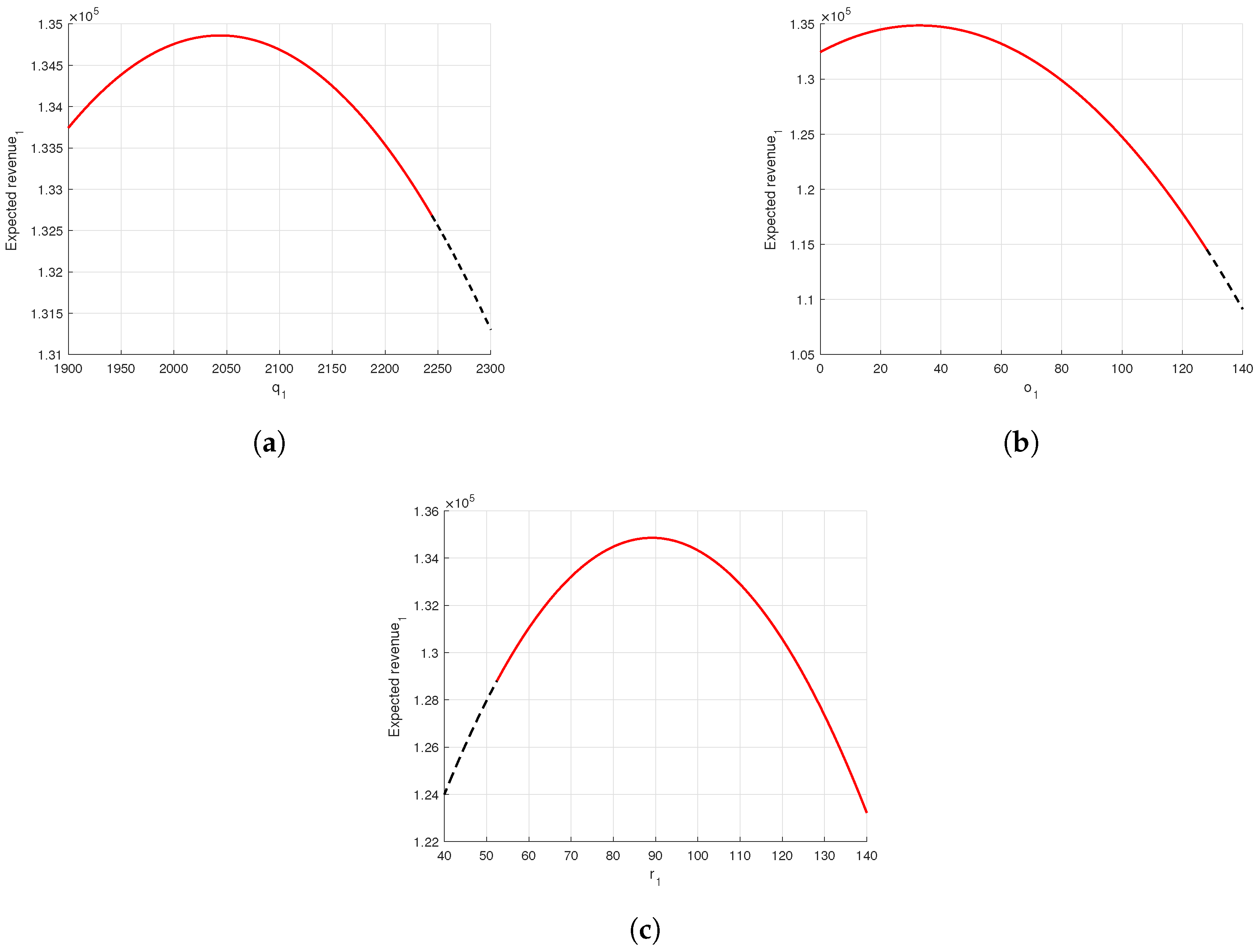
When the e-commerce platform adopts Policy I, the relationship between its expected revenue and the change in the three decision variables q, r, and o is shown in Figure 1. The highest point of the expected revenue function can be reached within the feasible region. When two of the variables q, r, and o are set to their optimal values, the red line in the figure below represents the change in expected revenue as the remaining variable changes.

Based on the exogenous market parameters we set, the values of various variables for the e-commerce platform under the three refund policies can be determined as shown in

Table 3. Optimal values.

Policies	${\mathit{q}}_{\mathit{i}}^{*}$	${\mathit{r}}_{\mathit{i}}^{*}$	${\mathit{o}}_{\mathit{i}}^{*}$	${\mathit{D}}_{\mathit{i}}$	${\mathit{D}}_{\mathit{i}2}$	${\mathit{D}}_{\mathit{i}3}$	${\mathit{R}}_{\mathit{i}}$	${\mathit{R}}_{\mathit{i}2}$	${\mathit{R}}_{\mathit{i}3}$	$\mathit{E}\left({\mathbf{\Pi }}_{\mathit{i}}(•)\right)$
Policy I	2043.7	89.1	32.8	1630.1	445.7	234.4	302.9	267.4	23.4	134,860.6
Policy II	1797.0	89.1	-	1395.7	445.7	-	279.4	267.4	-	107,396.3
Policy III	1574.5	-	32.8	1184.4	-	234.4	39.0	-	23.4	110,782.6

$i=1,2,3$ represent Policies I, II, and III, respectively.

, which illustrates that under these market conditions, the e-commerce platform can achieve greater expected revenue with Policy I, which offers both the basic refunds and refund guarantee option, while the platform’s revenue is lowest when adopting Policy II.

5.2. Sensitivity Analyses

In Section 5.1, we present the optimal values and expected revenues for the e-commerce platform under the three refund policies, finding that the platform achieves the highest revenue with Policy I. In this subsection, we will further investigate the impact of the deterioration rate and other parameters.

5.2.1. Effect of Deterioration Rate

Due to the perishability of fresh produce, the deterioration rate $\theta$ affects the product demand D, return quantity R, and order quantity q, as well as the optimal refund policy and the platform’s revenue. The following analysis examines the impact of the deterioration rate on the e-commerce platform under the three refund policies. First, we discuss how the platform’s expected revenue and order quantity are affected by $\theta$. Then, we study the impact of $\theta$ on the platform’s various decision variables. Finally, we analyze the effect of $\theta$ on the demand and return quantity. The corresponding results are shown in Figure 2 and Table 3.

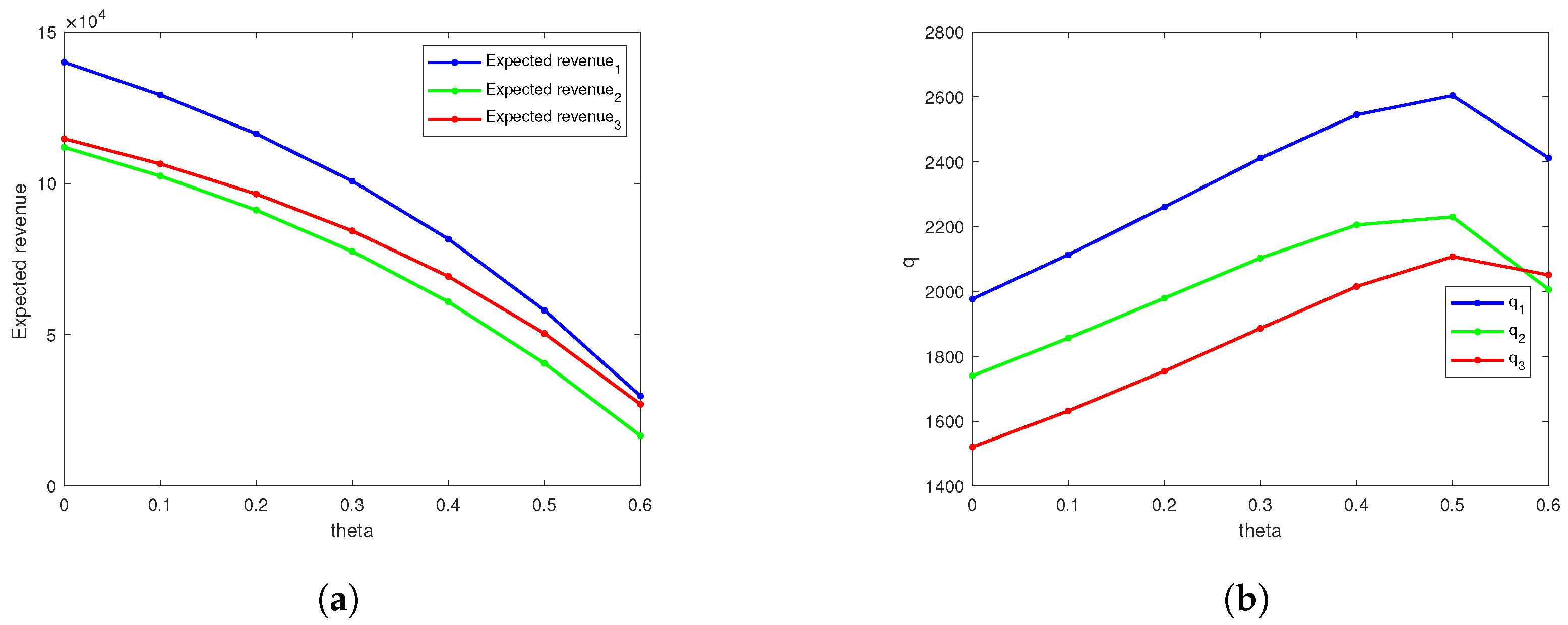
Figure 2a indicates that the expected revenue of the e-commerce platform is negatively correlated with the deterioration rate under three refund policies, consistent with the results of Corollary 2. Moreover, the platform always achieves the highest expected revenue under Policy I. However, while this indicates that as the deterioration rate increases, offering both basic refunds and refund guarantee option simultaneously yields more revenue for the platform compared to the other two refund policies, an increase in deterioration rate leads to a decrease in platform revenue. Therefore, managers need to invest efforts in preservation to reduce the deterioration rate and achieve more revenue.

Figure 2b shows that the order quantity of the e-commerce platforms under three refund policies initially increases and then decreases as the deterioration rate rises. In addition, the order quantity is higher under Policy I compared to Policies II and III. This curve is intuitive because some products spoil, and to meet demand, the platform needs to order more products to offset the spoiled ones. However, as the deterioration rate reaches a certain level, ordering too many products no longer aligns with the platform’s best interests. Therefore, the platform reduces the order quantity to minimize losses. Therefore, the optimal refund policy for fresh produce e-commerce platforms is to provide both basic refunds and refund guarantee option. When the deterioration rate is low, the platform should increase the order quantity as the deterioration rises. However, once the deterioration rate exceeds a certain threshold, the platform should reduce the order quantity.

The effect of deterioration rate on each variable is shown in

Table 4. Effects of deterioration rate on each variable.

$\mathit{\theta }$	${\mathit{q}}_1^{*}$	${\mathit{o}}_1^{*}$	${\mathit{r}}_1^{*}$	$\mathit{E}\left({\mathbf{\Pi }}_1(\mathit{q},\mathit{r},\mathit{o})\right)$	${\mathit{q}}_2^{*}$	${\mathit{r}}_2^{*}$	$\mathit{E}\left({\mathbf{\Pi }}_2(\mathit{q},\mathit{r})\right)$	${\mathit{q}}_3^{*}$	${\mathit{o}}_3^{*}$	$\mathit{E}\left({\mathbf{\Pi }}_3(\mathit{q},\mathit{o})\right)$
0.0	1977.0	31.5	91.3	140,016.5	1740.0	91.3	111,932.0	1520.3	31.5	114,751.2
0.1	2113.3	34.3	86.7	129,241.5	1856.2	86.7	102,458.2	1631.6	34.3	106,448.9
0.2	2260.3	37.8	80.9	116,358.7	1979.7	80.9	91,158.6	1754.6	37.8	96,476.2
0.3	2411.0	42.2	73.5	100,751.7	2103.1	73.5	77,516.2	1886.2	42.2	84,315.5
0.4	2545.0	48.2	63.6	81,616.5	2205.6	63.6	60,876.4	2015.4	48.2	69,258.6
0.5	2604.0	56.5	49.7	58,041.5	2230.0	49.7	40,557.0	2107.3	56.5	50,401.2
0.6	2411.3	69.0	28.8	29,710.3	2006.2	28.8	16,588.3	2050.8	69.0	26,976.2

.

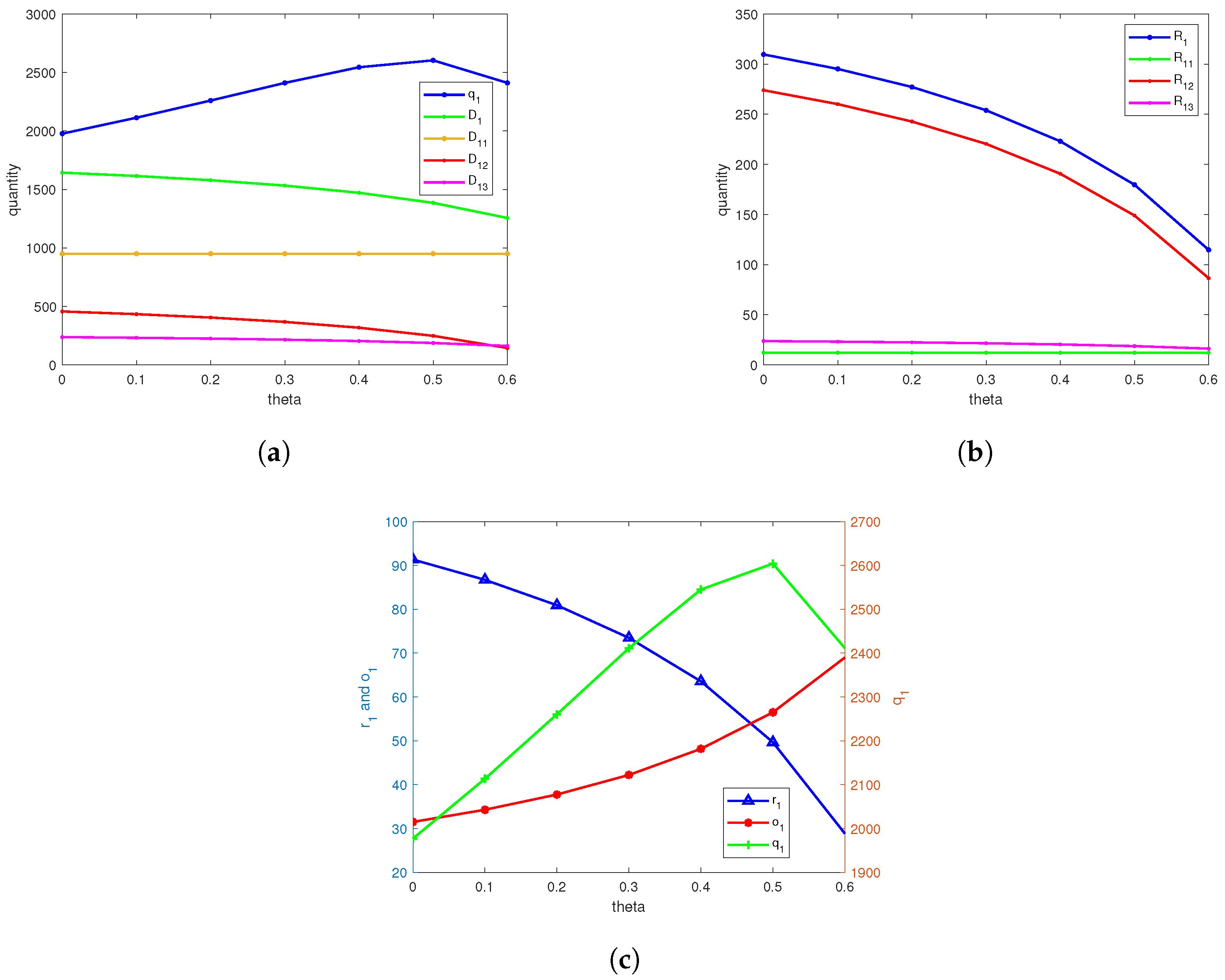
As shown in Table 4 and Figure 3c, when the deterioration rate is below a certain threshold, the greater the deterioration rate, the lower the basic refund price and expected revenue of the platform under the three refund policies. Conversely, the order quantity and the price of the refund guarantee option increase. Additionally, for the same deterioration rate, the platform’s expected profit and order quantity are highest under Policy I.

Therefore, when the deterioration rate is below a certain threshold, as the deterioration rate of fresh produce increases, the platform should offer a lower basic refund price, a higher order quantity, and a higher price for the refund guarantee option.

Next, we conduct a visual analysis of the impact of the deterioration rate on the demand and return quantity when the platform adopts Policy I. The corresponding results are shown in Figure 4.

Figure 3a shows the changes in q, $D_1$, $D_{11}$, $D_{12}$ and $D_{13}$ as $\theta$ varies. As $\theta$ increases, the demand decreases. This is because, with the increase in deterioration rate, the platform, aiming to protect its own profit, offers a lower basic refund price and a higher price for the refund guarantee option. Demand is positively correlated with the basic refund price and negatively correlated with the price of the refund guarantee option, leading to a decrease in demand. Secondly, the order quantity is higher than the demand, as the platform orders extra products to offset the spoiled portion. Finally, the figure shows that when the deterioration rate is low, the demand attracted by the basic refund policy is higher than that attracted by the option policy. When the deterioration rate is high, the opposite is true. This is because the basic refund policy deteriorates to such an extent that more people choose to purchase the refund guarantee option instead of the basic refund price, resulting in $D_{13}$ being higher than $D_{12}$.

Figure 3b shows the graph of $R_1$, $R_{11}$, $R_{12}$ and $R_{13}$ varying with $\theta$. As $\theta$ increases, the return quantity decreases. This is because with the increase in the deterioration rate, the platform offers a lower basic refund price and a higher price for the refund guarantee option. The return quantity is positively correlated with the basic refund price and negatively correlated with the price of the refund guarantee option, leading to a decrease in return quantity. Therefore, the platform can reduce the return quantity by appropriately lowering the basic refund price and increasing the refund guarantee option price.

5.2.2. Return Rate

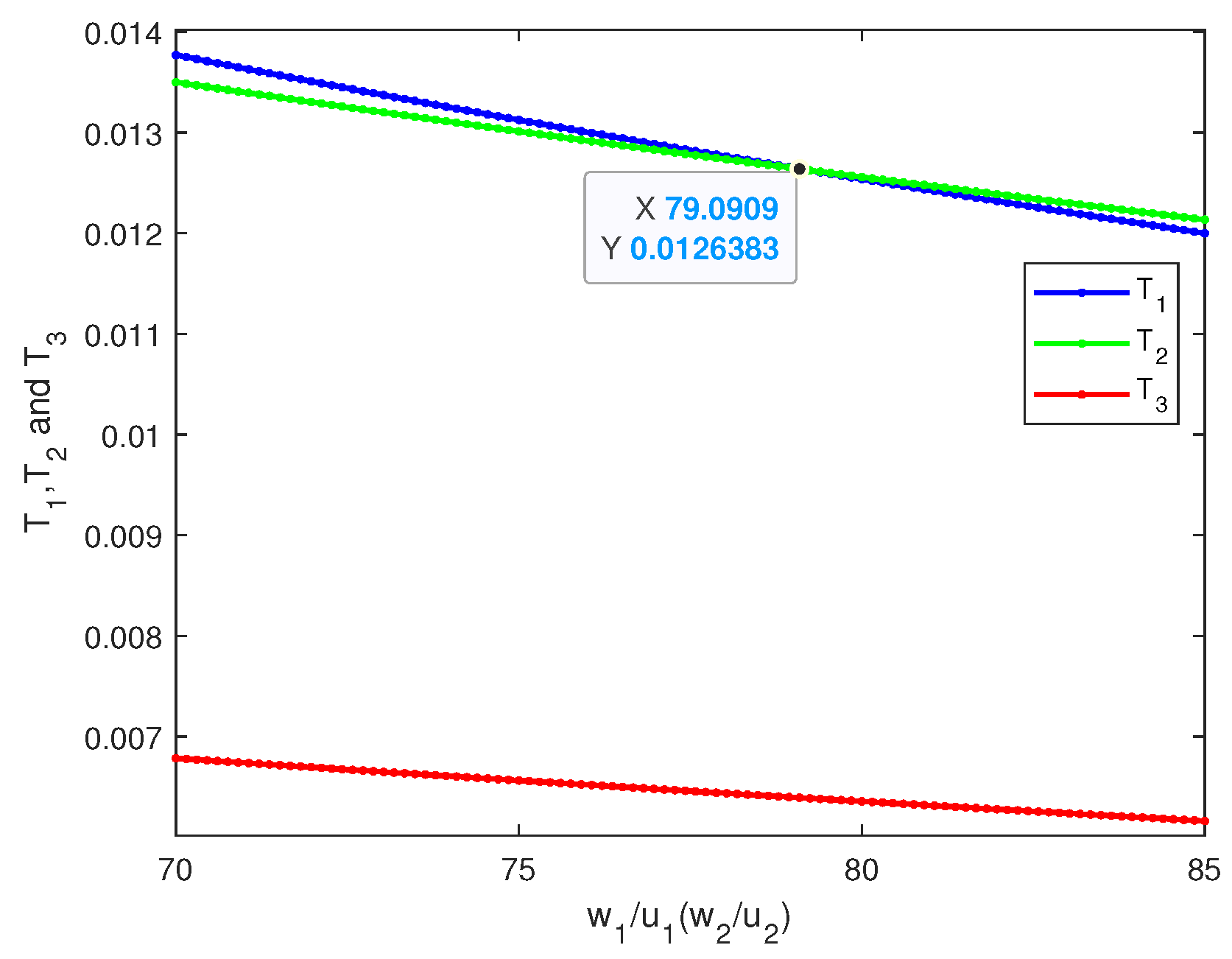
To compare and study the return rates under the three refund policies, let us assume that the sensitivity coefficient of demand to the basic refund policy ($w_1$) is equal to the sensitivity coefficient of demand to the refund guarantee option policy ($w_2$). Similarly, the sensitivity coefficient of return quantity to the basic refund policy ($u_1$) is equal to the sensitivity coefficient of the return quantity to the refund guarantee option policy ($u_2$). The refund policy also directly affects both the demand and return quantity, thereby influencing the return rate. Figure 4 compares the return rates under the three refund policies.

From Figure 4, it can be seen that when the ratio of demand to return quantity for the same refund policy sensitivity coefficient is greater than the ratio of the expected demand under the influence of a non-refund policy to the basic return quantity (475/6), the return rate of Policy I is lower than that of Policy II. Conversely, if the ratio is less, the conclusion is the opposite, which is consistent with the result of Property 1. At the same time, when the basic refund of Policy II minus the effective payment price of Policy III $r-(p-o)$ is greater than ${\displaystyle \frac{-R^{*}[D^{*}+w_2(p-o)]}{u_1{D}^{*}}}$, the return rate of Policy III is lower than that of Policy II, which is consistent with the result of Property 2. The return rate of Policy III is always lower than that of Policy I, which is consistent with the result of Property 3.

5.2.3. Effects of Changes in Sensitivity Coefficients

In this section, we analyze how demand and return quantity sensitivity coefficients for the basic refund policy and the refund guarantee option policy affect various decision variables and the platform’s expected revenue. Specifically, we examine how the optimal order quantity $q^{*}$, the optimal basic refund price $r^{*}$, the optimal refund guarantee option price $o^{*}$, and the platform’s expected revenue are influenced by $w_1$, $w_2$, $u_1$, and $u_2$. This analysis provides a reference for the platform to formulate refund policies and ordering decisions.

Table 5, Table 6, Table 7 and Table 8 indicate that, under the same parameter settings, the optimal order quantity and expected revenue for Policy I are always higher than those for Policy II and Policy III. Below, we will specifically analyze how $q^{*}$, $r^{*}$, and $o^{*}$ are influenced by $w_1$, $w_2$, $u_1$, and $u_2$.

(1)

Effects of the sensitivity of demand to the basic refund policy

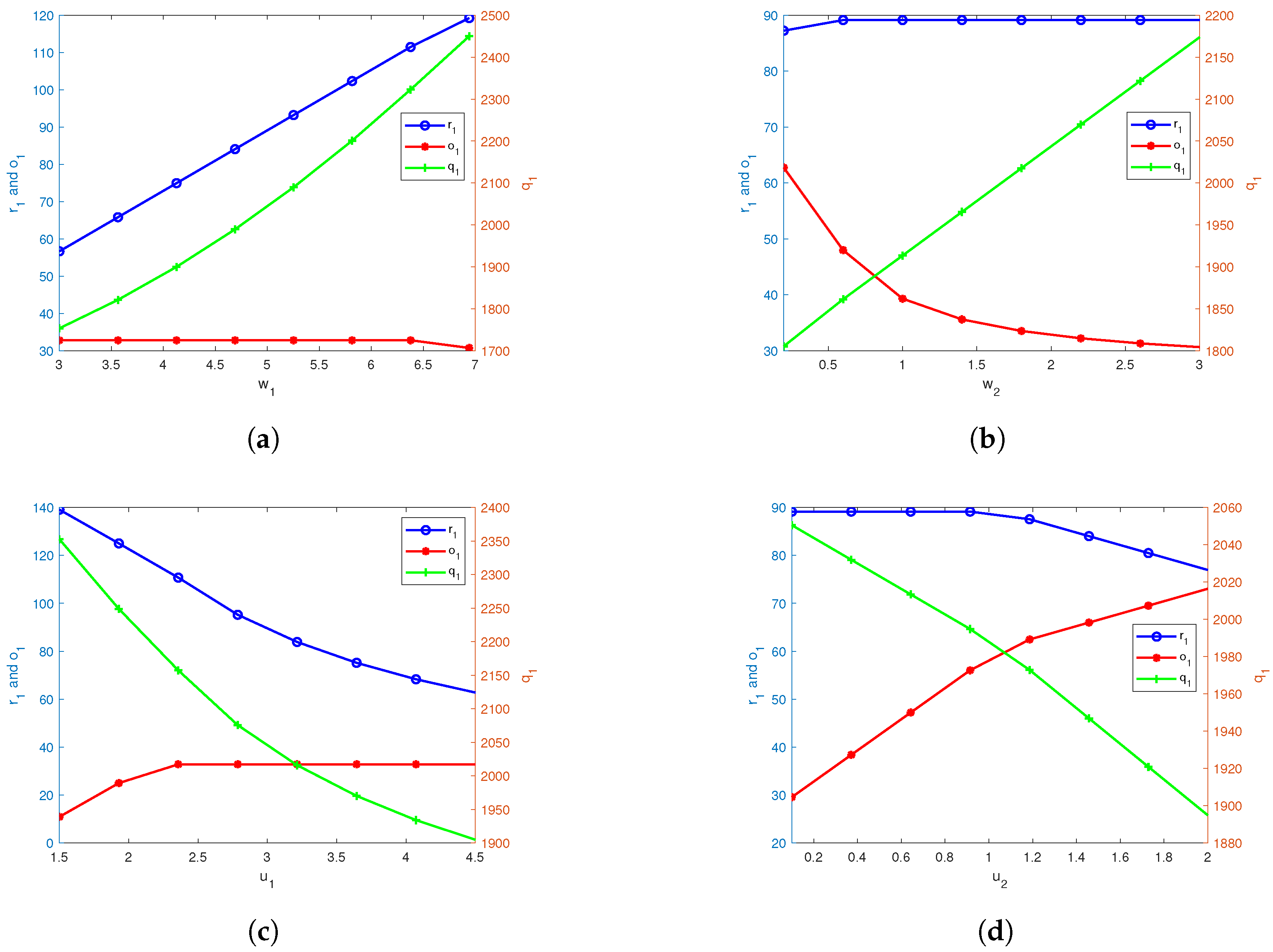
The data in Table 5 illustrate that in both Policy I and Policy II, as $w_1$ increases, the platform’s $q^{*}$ and $r^{*}$ also increase. Additionally, from Table 5 and Figure 5a, it can be seen that in Policy I, $o^{*}$ is not always independent of the sensitivity coefficient of demand to the basic refund policy. As $w_1$ increases, $o^{*}$ first stays constant and then decreases. This is because initially, $o^{*}$ is unaffected by $w_1$, but as $w_1$ continues to increase, $r^{*}$ gradually increases. To maintain the constraint $p-r^{*}-o^{*}\ge 0$, $o^{*}$ then decreases. At this point, the KKT point is converted from the solution in the first case in Section 4.2.1 to the solution in the second case. Specifically, when $w_1$ ranges from 3.0 to 6.4, the KKT point is obtained in the first scenario of Section 4.2.1, whereas when $w_1$ ranges from 5.8 to 6.9, the KKT point is obtained in the second scenario of Section 4.2.1.

In practice, if the consumer demand is more sensitive to the basic refund policy, the platform, after weighing the pros and cons, will choose to offer a better basic refund policy to attract more demand, leading to an increase in the platform’s order quantity. Furthermore, when consumer demand is highly sensitive to the basic refund policy, if the platform continues to offer a better basic refund policy without reducing the refund guarantee option price, consumers will not purchase the option when the basic refund policy is more favorable than the option policy. To encourage consumers to purchase the option, the platform will then lower the refund guarantee option price.

Therefore, when the platform adopts Policy I and Policy II, if consumer demand exhibits greater sensitivity to the basic refund policy, it should increase both the basic refund price and the order quantity. Furthermore, under Policy I, when the sensitivity coefficient surpasses a certain threshold, the platform should reduce the option price to optimize its policy.

Table 5. Results of the sensitivity of demand to the basic refund policy.

${\mathit{w}}_1$	${\mathit{q}}_1^{*}$	${\mathit{o}}_1^{*}$	${\mathit{r}}_1^{*}$	$\mathit{E}\left({\mathbf{\Pi }}_1(\mathit{q},\mathit{r},\mathit{o})\right)$	${\mathit{q}}_2^{*}$	${\mathit{r}}_2^{*}$	$\mathit{E}\left({\mathbf{\Pi }}_2(\mathit{q},\mathit{r})\right)$	${\mathit{q}}_3^{*}$	${\mathit{o}}_3^{*}$	$\mathit{E}\left({\mathbf{\Pi }}_3(\mathit{q},\mathit{o})\right)$
3.0	1753.5	32.8	56.7	120,661.9	1506.8	56.7	93,197.6	1574.5	32.8	110,782.6
3.6	1821.3	32.8	65.8	124,018.8	1574.6	65.8	96,554.5	1574.5	32.8	110,782.6
4.1	1900.0	32.8	75.0	127,876.2	1653.3	75.0	100,411.9	1574.5	32.8	110,782.6
4.7	1989.5	32.8	84.1	132,234.2	1742.8	84.1	104,769.9	1574.5	32.8	110,782.6
5.3	2089.8	32.8	93.2	137,092.8	1843.1	93.2	109,628.5	1574.5	32.8	110,782.6
5.8	2200.9	32.8	102.4	142,452.0	1954.2	102.4	114,987.7	1574.5	32.8	110,782.6
6.4	2322.9	32.8	111.5	148,311.8	2076.2	111.5	120,847.5	1574.5	32.8	110,782.6
6.9	2450.0	30.8	119.2	154,658.0	2209.0	120.6	127,207.9	1574.5	32.8	110,782.6

Table 5. Results of the sensitivity of demand to the basic refund policy.

${\mathit{w}}_1$	${\mathit{q}}_1^{*}$	${\mathit{o}}_1^{*}$	${\mathit{r}}_1^{*}$	$\mathit{E}\left({\mathbf{\Pi }}_1(\mathit{q},\mathit{r},\mathit{o})\right)$	${\mathit{q}}_2^{*}$	${\mathit{r}}_2^{*}$	$\mathit{E}\left({\mathbf{\Pi }}_2(\mathit{q},\mathit{r})\right)$	${\mathit{q}}_3^{*}$	${\mathit{o}}_3^{*}$	$\mathit{E}\left({\mathbf{\Pi }}_3(\mathit{q},\mathit{o})\right)$
3.0	1753.5	32.8	56.7	120,661.9	1506.8	56.7	93,197.6	1574.5	32.8	110,782.6
3.6	1821.3	32.8	65.8	124,018.8	1574.6	65.8	96,554.5	1574.5	32.8	110,782.6
4.1	1900.0	32.8	75.0	127,876.2	1653.3	75.0	100,411.9	1574.5	32.8	110,782.6
4.7	1989.5	32.8	84.1	132,234.2	1742.8	84.1	104,769.9	1574.5	32.8	110,782.6
5.3	2089.8	32.8	93.2	137,092.8	1843.1	93.2	109,628.5	1574.5	32.8	110,782.6
5.8	2200.9	32.8	102.4	142,452.0	1954.2	102.4	114,987.7	1574.5	32.8	110,782.6
6.4	2322.9	32.8	111.5	148,311.8	2076.2	111.5	120,847.5	1574.5	32.8	110,782.6
6.9	2450.0	30.8	119.2	154,658.0	2209.0	120.6	127,207.9	1574.5	32.8	110,782.6

(2)

Effects of the sensitivity of demand to the refund guarantee option policy

Table 6 shows that in both Policy I and Policy III, as $w_2$ increases, $q^{*}$ and the expected revenue under the corresponding policy increase, while $q^{*}$ decreases. Additionally, from Table 6 and Figure 5b, it can be seen that in Policy I, $r^{*}$ is not always independent of the demand sensitivity coefficient for the refund guarantee option policy. As $w_2$ increases, $r^{*}$ first increases and then remains unchanged. This is also influenced by the constraint $p-r^{*}-o^{*}\ge 0$, similar to the analysis in Table 5. At this point, the KKT point shifts from the solution in the second scenario described in Section 4.2.1 to the solution in the first scenario. Specifically, when $w_2$ is 0.2, the KKT point is obtained in the second scenario of Section 4.2.1, whereas when $w_2$ ranges from 0.6 to 3.0, the KKT point is obtained in the first scenario of Section 4.2.1. In practice, when the option price is high, if the basic refund policy is better than the option policy, consumers will be unwilling to purchase the option. Therefore, the basic refund price must be reduced. However, as the option price decreases, the option policy becomes more favorable than the basic refund policy, and it is no longer necessary to reduce the basic refund price. At this point, the basic refund price is unaffected by the sensitivity coefficient.

Therefore, when the platform adopts Policy I and Policy III, if consumer demand is increasingly sensitive to the refund guarantee option price, it should offer a lower refund guarantee option price and increase the order quantity. Additionally, under Policy I, when the sensitivity coefficient is relatively low, the platform should raise the basic refund price as the sensitivity increases. However, once the sensitivity coefficient surpasses a certain threshold, the basic refund price remains unchanged.

Table 6. Results of the sensitivity of demand to the refund guarantee option policy.

${\mathit{w}}_2$	${\mathit{q}}_1^{*}$	${\mathit{o}}_1^{*}$	${\mathit{r}}_1^{*}$	$\mathit{E}\left({\mathbf{\Pi }}_1(\mathit{q},\mathit{r},\mathit{o})\right)$	${\mathit{q}}_2^{*}$	${\mathit{r}}_2^{*}$	$\mathit{E}\left({\mathbf{\Pi }}_2(\mathit{q},\mathit{r})\right)$	${\mathit{q}}_3^{*}$	${\mathit{o}}_3^{*}$	$\mathit{E}\left({\mathbf{\Pi }}_3(\mathit{q},\mathit{o})\right)$
3.0	1753.5	32.8	56.7	120,661.9	1506.8	56.7	93,197.6	1574.5	32.8	110,782.6
0.2	1805.3	62.8	87.2	107,911.2	1797.0	89.1	107,396.3	1340.1	91.3	84,007.1
0.6	1861.4	48.0	89.1	113,640.9	1797.0	89.1	107,396.3	1392.2	48.0	89,562.9
1.0	1913.5	39.3	89.1	119,647.3	1797.0	89.1	107,396.3	1444.3	39.3	95,569.3
1.4	1965.5	35.6	89.1	125,718.2	1797.0	89.1	107,396.3	1496.4	35.6	101,640.2
1.8	2017.6	33.5	89.1	131,810.4	1797.0	89.1	107,396.3	1548.5	33.5	107,732.4
2.2	2069.7	32.2	89.1	137,912.5	1797.0	89.1	107,396.3	1600.5	32.2	113,834.5
2.6	2121.8	31.3	89.1	144,019.8	1797.0	89.1	107,396.3	1652.6	31.3	119,941.8
3.0	2173.9	30.6	89.1	150,130.2	1797.0	89.1	107,396.3	1704.7	30.6	126,052.2

Table 6. Results of the sensitivity of demand to the refund guarantee option policy.

${\mathit{w}}_2$	${\mathit{q}}_1^{*}$	${\mathit{o}}_1^{*}$	${\mathit{r}}_1^{*}$	$\mathit{E}\left({\mathbf{\Pi }}_1(\mathit{q},\mathit{r},\mathit{o})\right)$	${\mathit{q}}_2^{*}$	${\mathit{r}}_2^{*}$	$\mathit{E}\left({\mathbf{\Pi }}_2(\mathit{q},\mathit{r})\right)$	${\mathit{q}}_3^{*}$	${\mathit{o}}_3^{*}$	$\mathit{E}\left({\mathbf{\Pi }}_3(\mathit{q},\mathit{o})\right)$
3.0	1753.5	32.8	56.7	120,661.9	1506.8	56.7	93,197.6	1574.5	32.8	110,782.6
0.2	1805.3	62.8	87.2	107,911.2	1797.0	89.1	107,396.3	1340.1	91.3	84,007.1
0.6	1861.4	48.0	89.1	113,640.9	1797.0	89.1	107,396.3	1392.2	48.0	89,562.9
1.0	1913.5	39.3	89.1	119,647.3	1797.0	89.1	107,396.3	1444.3	39.3	95,569.3
1.4	1965.5	35.6	89.1	125,718.2	1797.0	89.1	107,396.3	1496.4	35.6	101,640.2
1.8	2017.6	33.5	89.1	131,810.4	1797.0	89.1	107,396.3	1548.5	33.5	107,732.4
2.2	2069.7	32.2	89.1	137,912.5	1797.0	89.1	107,396.3	1600.5	32.2	113,834.5
2.6	2121.8	31.3	89.1	144,019.8	1797.0	89.1	107,396.3	1652.6	31.3	119,941.8
3.0	2173.9	30.6	89.1	150,130.2	1797.0	89.1	107,396.3	1704.7	30.6	126,052.2

(3)

Effects of the sensitivity of return quantity to the basic refund policy

From Table 7, it can be seen that in both Policy I and Policy II, if $u_1$ increases, then $q^{*}$, $r^{*}$, and the expected revenue under the corresponding policy decrease. Additionally, from Table 7 and Figure 5c, it can be observed that in Policy I, $o^{*}$ is not always independent of the sensitivity coefficient of return quantity to the basic refund policy. As $u_1$ increases, $o^{*}$ first increases and then remains constant, also influenced by the constraint $p-r^{*}-o^{*}\ge 0$. At this point, the KKT point transitions from the solution in the second scenario of Section 4.2.1 to the solution in the first scenario. Specifically, when $u_1$ is between 1.5 and 1.9, the KKT point is obtained in the second scenario of Section 4.2.1, whereas when $u_1$ is between 2.4 and 4.5, the KKT point is obtained in the first scenario of Section 4.2.1. In fact, if consumers are more sensitive to the basic refund policy in terms of return quantity, the platform will choose to offer a worse basic refund policy after weighing the pros and cons to reduce the return quantity caused by the basic refund policy.

Therefore, when the platform adopts Policy I and Policy II, if consumer returns are more sensitive to the basic refund policy, the platform should reduce the market order quantity and offer a lower basic refund price. Additionally, under Policy I, when the sensitivity coefficient is relatively low, the platform should set a lower refund guarantee option price. However, once this sensitivity coefficient exceeds a certain threshold, the refund guarantee option price remains unchanged as the sensitivity increases.

Table 7. Results of the sensitivity of return quantity to the basic refund policy.

${\mathit{u}}_1$	${\mathit{q}}_1^{*}$	${\mathit{o}}_1^{*}$	${\mathit{r}}_1^{*}$	$\mathit{E}\left({\mathbf{\Pi }}_1(\mathit{q},\mathit{r},\mathit{o})\right)$	${\mathit{q}}_2^{*}$	${\mathit{r}}_2^{*}$	$\mathit{E}\left({\mathbf{\Pi }}_2(\mathit{q},\mathit{r})\right)$	${\mathit{q}}_3^{*}$	${\mathit{o}}_3^{*}$	$\mathit{E}\left({\mathbf{\Pi }}_3(\mathit{q},\mathit{o})\right)$
1.5	2352.6	10.9	139.1	151,262.3	2117.3	150.0	125,534.6	1574.5	32.8	110,782.6
1.9	2248.9	25.0	125.0	144,943.2	2028.4	133.1	117,727.9	1574.5	32.8	110,782.6
2.4	2157.3	32.8	110.7	139,920.8	1910.6	110.7	112,456.5	1574.5	32.8	110,782.6
2.8	2075.7	32.8	95.2	136,284.5	1829.0	95.2	108,820.3	1574.5	32.8	110,782.6
3.2	2015.9	32.8	83.9	133,629.4	1769.2	83.9	106,165.1	1574.5	32.8	110,782.6
3.6	1970.2	32.8	75.2	131,609.1	1723.4	75.2	104,144.8	1574.5	32.8	110,782.6
4.1	1934.0	32.8	68.3	130,023.1	1687.3	68.3	102,558.9	1574.5	32.8	110,782.6
4.5	1904.8	32.8	62.8	128,747.4	1658.1	62.8	101,283.1	1574.5	32.8	110,782.6

Table 7. Results of the sensitivity of return quantity to the basic refund policy.

${\mathit{u}}_1$	${\mathit{q}}_1^{*}$	${\mathit{o}}_1^{*}$	${\mathit{r}}_1^{*}$	$\mathit{E}\left({\mathbf{\Pi }}_1(\mathit{q},\mathit{r},\mathit{o})\right)$	${\mathit{q}}_2^{*}$	${\mathit{r}}_2^{*}$	$\mathit{E}\left({\mathbf{\Pi }}_2(\mathit{q},\mathit{r})\right)$	${\mathit{q}}_3^{*}$	${\mathit{o}}_3^{*}$	$\mathit{E}\left({\mathbf{\Pi }}_3(\mathit{q},\mathit{o})\right)$
1.5	2352.6	10.9	139.1	151,262.3	2117.3	150.0	125,534.6	1574.5	32.8	110,782.6
1.9	2248.9	25.0	125.0	144,943.2	2028.4	133.1	117,727.9	1574.5	32.8	110,782.6
2.4	2157.3	32.8	110.7	139,920.8	1910.6	110.7	112,456.5	1574.5	32.8	110,782.6
2.8	2075.7	32.8	95.2	136,284.5	1829.0	95.2	108,820.3	1574.5	32.8	110,782.6
3.2	2015.9	32.8	83.9	133,629.4	1769.2	83.9	106,165.1	1574.5	32.8	110,782.6
3.6	1970.2	32.8	75.2	131,609.1	1723.4	75.2	104,144.8	1574.5	32.8	110,782.6
4.1	1934.0	32.8	68.3	130,023.1	1687.3	68.3	102,558.9	1574.5	32.8	110,782.6
4.5	1904.8	32.8	62.8	128,747.4	1658.1	62.8	101,283.1	1574.5	32.8	110,782.6

(4)

Effects of the sensitivity of return quantity to the refund guarantee option policy

From Table 8, it can be seen that in both Policy I and Policy III, if $u_2$ increases, then $q^{*}$ and the expected revenue under the corresponding policy decrease, while $o^{*}$ increases. Additionally, from Table 8 and Figure 5d, it can be observed that in Policy I, $r^{*}$ is not always independent of the sensitivity coefficient of the return quantity to the basic refund policy. As $u_2$ increases, $q^{*}$ first remains constant and then decreases, also constrained by the constraint $p-r^{*}-o^{*}\ge 0$. At this point, the KKT point transitions from the solution in the first scenario of Section 4.2.1 to the solution in the second scenario. Specifically, when $u_2$ is between 0.1 and 0.9, the KKT point is obtained in the first scenario of Section 4.2.1, whereas when $u_2$ is between 1.2 and 2.0, the KKT point is obtained in the second scenario of Section 4.2.1. In fact, if the consumers’ return quantity is more sensitive to the return guarantee option price, a lower option price will attract more returns. To reduce the return quantity, the platform will offer a worse return guarantee option policy.

Therefore, when the platform adopts Policy I and Policy III, if consumer returns are more sensitive to the refund guarantee option price, the platform should reduce the market order quantity and offer a higher refund guarantee option price. Additionally, under Policy I, when the sensitivity coefficient is relatively low, the platform should maintain a higher basic refund price. However, once the sensitivity coefficient exceeds a certain threshold, the platform should decrease the basic refund price as the sensitivity increases.

Table 8. Results of the sensitivity of the return quantity to the refund guarantee option policy.

${\mathit{u}}_2$	${\mathit{q}}_1^{*}$	${\mathit{o}}_1^{*}$	${\mathit{r}}_1^{*}$	$\mathit{E}\left({\mathbf{\Pi }}_1(\mathit{q},\mathit{r},\mathit{o})\right)$	${\mathit{q}}_2^{*}$	${\mathit{r}}_2^{*}$	$\mathit{E}\left({\mathbf{\Pi }}_2(\mathit{q},\mathit{r})\right)$	${\mathit{q}}_3^{*}$	${\mathit{o}}_3^{*}$	$\mathit{E}\left({\mathbf{\Pi }}_3(\mathit{q},\mathit{o})\right)$
0.1	2050.5	29.6	89.1	136,405.1	1797.0	89.1	107,396.3	1581.3	29.6	112,327.1
0.4	2031.9	38.4	89.1	132,311.2	1797.0	89.1	107,396.3	1562.8	38.4	108,233.2
0.6	2013.4	47.2	89.1	128,528.5	1797.0	89.1	107,396.3	1544.2	47.2	104,450.5
0.9	1994.8	56.0	89.1	125,057.0	1797.0	89.1	107,396.3	1525.6	56.0	100,979.0
1.2	1972.9	62.5	87.5	121,877.7	1797.0	89.1	107,396.3	1507.1	64.9	97,818.9
1.5	1946.9	66.0	84.0	118,851.0	1797.0	89.1	107,396.3	1488.5	73.7	94,970.0
1.7	1920.9	69.5	80.5	115,948.7	1797.0	89.1	107,396.3	1469.9	82.5	92,432.4
2.0	1894.9	73.0	77.0	113,170.9	1797.0	89.1	107,396.3	1451.3	91.3	90,206.0

Table 8. Results of the sensitivity of the return quantity to the refund guarantee option policy.

${\mathit{u}}_2$	${\mathit{q}}_1^{*}$	${\mathit{o}}_1^{*}$	${\mathit{r}}_1^{*}$	$\mathit{E}\left({\mathbf{\Pi }}_1(\mathit{q},\mathit{r},\mathit{o})\right)$	${\mathit{q}}_2^{*}$	${\mathit{r}}_2^{*}$	$\mathit{E}\left({\mathbf{\Pi }}_2(\mathit{q},\mathit{r})\right)$	${\mathit{q}}_3^{*}$	${\mathit{o}}_3^{*}$	$\mathit{E}\left({\mathbf{\Pi }}_3(\mathit{q},\mathit{o})\right)$
0.1	2050.5	29.6	89.1	136,405.1	1797.0	89.1	107,396.3	1581.3	29.6	112,327.1
0.4	2031.9	38.4	89.1	132,311.2	1797.0	89.1	107,396.3	1562.8	38.4	108,233.2
0.6	2013.4	47.2	89.1	128,528.5	1797.0	89.1	107,396.3	1544.2	47.2	104,450.5
0.9	1994.8	56.0	89.1	125,057.0	1797.0	89.1	107,396.3	1525.6	56.0	100,979.0
1.2	1972.9	62.5	87.5	121,877.7	1797.0	89.1	107,396.3	1507.1	64.9	97,818.9
1.5	1946.9	66.0	84.0	118,851.0	1797.0	89.1	107,396.3	1488.5	73.7	94,970.0
1.7	1920.9	69.5	80.5	115,948.7	1797.0	89.1	107,396.3	1469.9	82.5	92,432.4
2.0	1894.9	73.0	77.0	113,170.9	1797.0	89.1	107,396.3	1451.3	91.3	90,206.0

(5)

Effects of sensitivity coefficients on expected revenue

Furthermore, we utilize three-dimensional graphs to analyze how the expected revenue is influenced by various sensitivity coefficients when adopting Policy I on the platform. The corresponding results are presented in Figure 6. From the graphs, it is evident that the expected revenue increases as the sensitivity coefficient of demand to the basic refund policy ($w_1$) and the sensitivity coefficient of demand to the refund guarantee option policy ($w_2$) increase, while it decreases as the sensitivity coefficients of the return quantity to the basic refund policy ($u_1$) and the sensitivity coefficients of the return quantity to the refund guarantee option policy ($u_2$), deterioration rate ($\theta$), and price sensitivity coefficients (b) increase. These findings are consistent with the theoretical conclusions outlined in Section 4.4.

(6)

Effects of market uncertainty

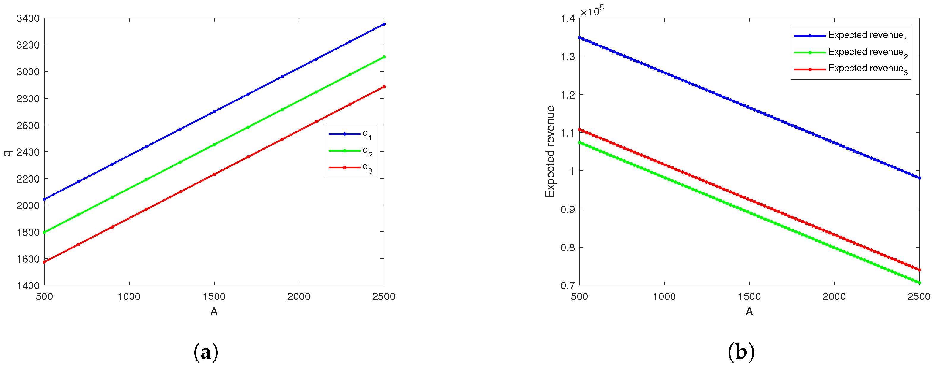
Finally, we analyze the impact of market uncertainty on the platform’s decision variables and expected revenues under three refund policies. Figure 7a and

Table 9. Results of the market uncertainty.

A	${\mathit{q}}_1^{*}$	${\mathit{o}}_1^{*}$	${\mathit{r}}_1^{*}$	$\mathit{E}\left({\mathbf{\Pi }}_1(\mathit{q},\mathit{r},\mathit{o})\right)$	${\mathit{q}}_2^{*}$	${\mathit{r}}_2^{*}$	$\mathit{E}\left({\mathbf{\Pi }}_2(\mathit{q},\mathit{r})\right)$	${\mathit{q}}_3^{*}$	${\mathit{o}}_3^{*}$	$\mathit{E}\left({\mathbf{\Pi }}_3(\mathit{q},\mathit{o})\right)$
500.0	2043.7	32.8	89.1	134,860.6	1797.0	89.1	107,396.3	1574.5	32.8	110,782.6
700.0	2174.8	32.8	89.1	131,187.9	1928.1	89.1	103,723.7	1705.6	32.8	107,109.9
900.0	2305.9	32.8	89.1	127,515.3	2059.2	89.1	100,051.0	1836.7	32.8	103,437.3
1100.0	2437.0	32.8	89.1	123,842.6	2190.3	89.1	96,378.3	1967.8	32.8	99,764.6
1300.0	2568.1	32.8	89.1	120,169.9	2321.4	89.1	92,705.7	2099.0	32.8	96,091.9
1500.0	2699.2	32.8	89.1	116,497.3	2452.5	89.1	89,033.0	2230.1	32.8	92,419.3
1700.0	2830.4	32.8	89.1	112,824.6	2583.7	89.1	85,360.3	2361.2	32.8	88,746.6
1900.0	2961.5	32.8	89.1	109,151.9	2714.8	89.1	81,687.7	2492.3	32.8	85,073.9

demonstrate that increasing market uncertainty (A) does not affect the prices of the basic refund and refund guarantee option, but the platform will increase the order quantity to address market fluctuations. Nevertheless, the platform’s expected revenues will decrease as shown in Figure 7b.

6. Conclusions and Management Insights

6.1. Conclusions

This study is based on three typical refund policies: Policy I, which combines both basic refund and refund guarantee option policies; Policy II, which offers only a basic refund; and Policy III, which provides only a refund guarantee option. We develop a model for ordering and refund decisions for fresh produce e-commerce platforms under uncertain market demand to explore the optimal ordering quantity, basic refund price, and refund guarantee option price. The key findings are as follows:

(1) We derive the optimal basic refund price, optimal refund guarantee option price, and optimal order quantity for the e-commerce platform under three refund policies. With the same parameter settings, offering both basic refund and refund guarantee option (Policy I) yields the highest order quantity and expected revenue.

(2) When the sensitivity coefficients of demand and return quantity to the basic refund policy and refund guarantee option policy are equal, the following return rate properties emerge: (1) If the ratio of the demand to return quantity sensitivity coefficients for the refund policy exceeds the ratio of the expected demand affected by the non-refund policy to the basic return quantity, Policy I has a lower return rate than Policy II. (2) Policy III consistently has a lower return rate than Policy I. (3) If the difference between the basic refund price of Policy II and the effective payment price of Policy III exceeds a certain threshold, Policy III’s return rate will be lower than that of Policy II under the same conditions.

(3) As the sensitivity coefficients of demand to the two refund policies increase, the platform’s expected revenue increases. Conversely, as the sensitivity coefficients of return, deterioration rate, and price increase, the platform’s expected revenue decreases.

(4) As the deterioration rate increases, the platform should reduce basic refunds, increase refund guarantee option prices, and adjust order quantities. This leads to decreased demand, return quantities, and expected revenue. When spoilage exceeds a certain threshold, order quantities decrease.

(5) Under Policy I, increased sensitivity of demand to the basic refund policy raises the order quantity and the basic refund, while initially keeping the option price stable and then decreasing it. Increased sensitivity of returns to the basic refund policy decreases the order quantity and the basic refund, with the option price rising initially and then stabilizing. Increased sensitivity of demand to the refund guarantee option policy increases the order quantity and decreases the option price, with the basic refund first increasing and then stabilizing. Increased sensitivity of returns to the refund guarantee option policy decreases the order quantity and increases the option price, while the basic refund first remains stable and then decreases.

Under Policy II, both the basic refund price and order quantity increase with higher sensitivity of demand to the basic refund policy, while both decrease with higher sensitivity of returns to the basic refund.

Under Policy III, the increased sensitivity of demand to the refund guarantee option policy raises the order quantity and lowers the option price, while increased sensitivity of returns decreases the order quantity and raises the option price.

(6) Increased market uncertainty does not affect the basic refund and refund guarantee option prices, but it leads to higher order quantities and lower expected revenue.

6.2. Managerial Insights

To fully apply the theoretical results of this paper, the following five managerial insights are proposed to help fresh produce e-commerce platforms optimize their operations and improve product utilization.

(1) To maximize revenue, the optimal policy is to adopt both the basic refund and refund guarantee option policies. However, to minimize return rates, adjustments are needed. Specifically, if the ratio of the demand and return sensitivity to the refund policy exceeds the ratio of the expected demand under the no-refund policy to the basic refund price, and the difference between the optimal basic refund price in Policy II and the effective payment price in Policy III exceeds a threshold, adopting only the refund guarantee option policy is recommended. Otherwise, the platform should adjust its policy based on the three key properties discussed in this paper.

(2) When the platform adopts Policy I, as consumer demand becomes more sensitive to the basic refund price, the platform should increase order quantities and raise the basic refund price. If this sensitivity surpasses a threshold, the platform should raise the refund guarantee option price. As consumer demand becomes more sensitive to the refund guarantee option price, the platform should increase order quantities, lower the option price, and raise the basic refund price; if this sensitivity exceeds a threshold, the basic refund should remain constant. As consumer returns become more sensitive to the basic refund price, the platform should reduce both order quantities and the basic refund while increasing the option price; if this sensitivity surpasses a threshold, the option price should remain unchanged. Finally, as consumer returns become more sensitive to the refund guarantee option price, the platform should reduce order quantities, increase the option price, and decrease the basic refund price if this sensitivity exceeds a threshold.

When the platform adopts Policy II, as consumer demand becomes more sensitive to the basic refund price, the platform should increase both the basic refund price and order quantity. Conversely, as consumer returns become more sensitive to the basic refund price, the recommendations are reversed.

When the platform adopts Policy III, as consumer demand becomes more sensitive to the refund guarantee option price, the platform should offer a lower refund guarantee option price and increase the order quantity. Conversely, as consumer returns become more sensitive to the refund guarantee option price, the recommendations are reversed.

(3) As the deterioration rate increases, the platform should offer lower basic refunds, higher option prices, and larger order quantities. However, if the deterioration rate surpasses a certain threshold, the platform should reduce order quantities.

(4) As market uncertainty increases, the platform should moderately increase order quantities to address market fluctuations and reduce the risk of potential supply–demand imbalances

This study is practically significant. Overstocking fresh produce pressures producers and e-commerce platforms by occupying inventory space, increasing deterioration rates, and causing asset depreciation. Excess spoilage also leads to resource waste and environmental impact. Accurate demand forecasting, optimized ordering, and suitable refund policies can reduce waste and improve produce utilization.

This study acknowledges several limitations. First, the model constructed in this paper is based on specific assumptions, and optimal decisions may vary depending on the characteristics of different products and market conditions. E-commerce platforms should adapt their policies accordingly, based on the particular context. Secondly, this study does not account for the dynamic nature of the deterioration rate. In practice, fresh products deteriorate within a limited time frame, and the rate of deterioration is time-dependent. Furthermore, the current analysis only considers demand uncertainty without incorporating the stochastic nature of return quantity. Future research could explore the following directions: (1) investigate dynamic deterioration rate to better reflect real-world conditions; (2) incorporate the stochasticity of return quantity and examine the joint stochasticity of production and demand, thereby offering a more comprehensive reflection of market dynamics; and (3) while this paper focuses on optimal decisions and revenues for fresh produce e-commerce platforms, future studies could expand to explore management coordination within the three-tier supply chain, involving fresh produce producers, e-commerce platforms, and consumers, to achieve better management alignment.

References

1. Wang, C.; Chen, X. Option pricing and coordination in the fresh produce supply chain with portfolio contracts. Ann. Oper. Res. 2017, 248, 471–491. [Google Scholar] [CrossRef]
2. Allianz Trade. Agrifood Industry 2023 Outlook. Available online: https://www.allianz-trade.com/en_SG/resources/reports/agrifood-report-2023.html (accessed on 9 March 2023).
3. Emarketer. US Internet Users Whose Concern About Temperature/Freshness of Fresh/Frozen Food Items Is the Reason They Have Not Ordered Them Online for Home Delivery. Available online: https://www.emarketer.com/chart/230850/us-internet-users-whose-concern-about-temperaturefreshness-of-fresh-frozen-food-items-reason-they-have-not-ordered-them-online-home-delivery-aug-2019-of-respondentsby-age (accessed on 20 November 2023).
4. Fan, H.; Khouja, M.; Zhou, J. Design of win-win return policies for online retailers. Eur. J. Oper. Res. 2022, 301, 675–693. [Google Scholar] [CrossRef]
5. Heiman, A.; McWilliams, B.; Zilberman, D. Demonstrations and money-back guarantees: Market mechanisms to reduce uncertainty. J. Bus. Res. 2001, 54, 71–84. [Google Scholar] [CrossRef]
6. Suwelack, T.; Hogreve, J.; Hoyer, W.D. Understanding money-back guarantees: Cognitive, affective, and behavioral outcomes. J. Retail. 2011, 87, 462–478. [Google Scholar] [CrossRef]
7. Fresh Market. Our No Hassle Return Policy. Available online: https://www.thefreshmarket.com/return-policy (accessed on 19 March 2023).
8. Amazon. Spilled or Damaged Amazon Fresh Items. Available online: https://www.amazon.com/gp/help/customer/display.html?nodeId=GKVRR7EEVPXCG9BM (accessed on 20 March 2023).
9. Zhang, X.; Chen, H.; Hu, J.; Ma, C.; Shi, W. Optimal showroom service strategy and power structure for retailers considering consumer return. Discret. Dyn. Nat. Soc. 2021, 2021, 4598341. [Google Scholar] [CrossRef]
10. Ülkü, M.A.; Dailey, L.C.; Yayla-Küllü, H.M. Serving fraudulent consumers? The impact of return policies on retailer’s profitability. Serv. Sci. 2013, 5, 296–309. [Google Scholar] [CrossRef]
11. Chen, J.; Yu, B.; Chen, B.; Liu, Z. Lenient vs. stringent returns policies in the presence of fraudulent returns: The role of customers’ fairness perceptions. Omega 2023, 117, 102843. [Google Scholar] [CrossRef]
12. Dye, C.Y.; Ouyang, L.Y.; Hsieh, T.P. Inventory and pricing strategies for deteriorating items with shortages: A discounted cash flow approach. Comput. Ind. Eng. 2007, 52, 29–40. [Google Scholar] [CrossRef]
13. Feng, L. Dynamic pricing, quality investment, and replenishment model for perishable items. Int. Trans. Oper. Res. 2019, 26, 1558–1575. [Google Scholar] [CrossRef]
14. Kayikci, Y.; Demir, S.; Mangla, S.K.; Subramanian, N.; Koc, B. Data-driven optimal dynamic pricing strategy for reducing perishable food waste at retailers. J. Clean. Prod. 2022, 344, 131068. [Google Scholar] [CrossRef]
15. Scholz, M.; Kulko, R.D. Dynamic pricing of perishable food as a sustainable business model. Br. Food J. 2022, 124, 1609–1621. [Google Scholar] [CrossRef]
16. Pasternack, B.A. Optimal pricing and return policies for perishable commodities. Mark. Sci. 1985, 4, 166–176. [Google Scholar] [CrossRef]
17. Li, Y.; Li, K.; Gharehgozli, A. Optimal return and refund policies for perishable food items with online grocery shopping. Int. J. Prod. Res. 2023, 61, 6519–6532. [Google Scholar] [CrossRef]
18. Zhang, Q.; Chen, J.; Chen, B. Information strategy in a supply chain under asymmetric customer returns information. Transp. Res. Part Logist. Transp. Rev. 2021, 155, 102511. [Google Scholar] [CrossRef]
19. Chen, J.; Bell, P.C. The impact of customer returns on pricing and order decisions. Eur. J. Oper. Res. 2009, 195, 280–295. [Google Scholar] [CrossRef]
20. Ghoreishi, M.; Weber, G.W.; Mirzazadeh, A. An inventory model for non-instantaneous deteriorating items with partial backlogging, permissible delay in payments, inflation-and selling price-dependent demand and customer returns. Ann. Oper. Res. 2015, 226, 221–238. [Google Scholar] [CrossRef]
21. Li, Y.; Xu, L.; Li, D. Examining relationships between the return policy, product quality, and pricing strategy in online direct selling. Int. J. Prod. Econ. 2013, 144, 451–460. [Google Scholar] [CrossRef]
22. Che, Y.K. Customer return policies for experience goods. J. Ind. Econ. 1996, 44, 17–24. [Google Scholar] [CrossRef]
23. Batarfi, R.; Jaber, M.Y.; Aljazzar, S.M. A profit maximization for a reverse logistics dual-channel supply chain with a return policy. Comput. Ind. Eng. 2017, 106, 58–82. [Google Scholar] [CrossRef]
24. Wood, S.L. Remote purchase environments: The influence of return policy leniency on two-stage decision processes. J. Mark. Res. 2001, 38, 157–169. [Google Scholar] [CrossRef]
25. Mukhopadhyay, S.K.; Setoputro, R. Optimal return policy and modular design for build-to-order products. J. Oper. Manag. 2005, 23, 496–506. [Google Scholar] [CrossRef]
26. Li, D.; Chen, J.; Liao, Y. Optimal decisions on prices, order quantities, and returns policies in a supply chain with two-period selling. Eur. J. Oper. Res. 2021, 290, 1063–1082. [Google Scholar] [CrossRef]
27. Ma, Y.; Zhang, C.; Li, Y. Strategies for the retail platform to counteract match uncertainty: Virtual showroom and return or exchange policy. Comput. Ind. Eng. 2023, 176, 108832. [Google Scholar] [CrossRef]
28. Chen, H.W. Improving supply quality through the store-initiated returns in wholesale supply chains. Int. J. Prod. Econ. 2023, 261, 108891. [Google Scholar] [CrossRef]
29. Zhang, Z.; Liu, S.; Niu, B. Coordination mechanism of dual-channel closed-loop supply chains considering product quality and return. J. Clean. Prod. 2020, 248, 119273. [Google Scholar] [CrossRef]
30. Ketzenberg, M.E.; Abbey, J.D.; Heim, G.R.; Kumar, S. Assessing customer return behaviors through data analytics. J. Oper. Manag. 2020, 66, 622–645. [Google Scholar] [CrossRef]
31. Bandi, C.; Moreno, A.; Ngwe, D.; Xu, Z. Opportunistic returns and dynamic pricing: Empirical evidence from online retailing in emerging markets. In Working Paper 19-030; Harvard Business School: Boston, MA, USA, 2018. [Google Scholar]
32. Hess, J.D.; Chu, W.; Gerstner, E. Controlling product returns in direct marketing. Mark. Lett. 1996, 7, 307–317. [Google Scholar] [CrossRef]
33. Khouja, M.; Hammami, R. Optimizing price, order quantity, and return policy in the presence of consumer opportunistic behavior for online retailers. Eur. J. Oper. Res. 2023, 309, 683–703. [Google Scholar] [CrossRef]
34. Akçay, Y.; Boyacı, T.; Zhang, D. Selling with money-back guarantees: The impact on prices, quantities, and retail profitability. Prod. Oper. Manag. 2013, 22, 777–791. [Google Scholar] [CrossRef]
35. Mukhopadhyay, S.K.; Setoputro, R. Reverse logistics in e-business: Optimal price and return policy. Int. J. Phys. Distrib. Logist. Manag. 2004, 34, 70–89. [Google Scholar] [CrossRef]
36. Su, X. Consumer returns policies and supply chain performance. Manuf. Serv. Oper. Manag. 2009, 11, 595–612. [Google Scholar] [CrossRef]
37. Wang, C.; Chen, J.; Chen, X. The impact of customer returns and bidirectional option contract on refund price and order decisions. Eur. J. Oper. Res. 2019, 274, 267–279. [Google Scholar] [CrossRef]
38. Mandal, P.; Basu, P.; Saha, K. Forays into omnichannel: An online retailer’s strategies for managing product returns. Eur. J. Oper. Res. 2021, 292, 633–651. [Google Scholar] [CrossRef]
39. Gao, F.; Agrawal, V.V.; Cui, S. The effect of multichannel and omnichannel retailing on physical stores. Manag. Sci. 2022, 68, 809–826. [Google Scholar] [CrossRef]
40. Nageswaran, L.; Cho, S.H.; Scheller-Wolf, A. Consumer return policies in omnichannel operations. Manag. Sci. 2020, 66, 5558–5575. [Google Scholar] [CrossRef]
41. Qin, Y.; Wang, J.; Wei, C. Joint pricing and inventory control for fresh produce and foods with quality and physical quantity deteriorating simultaneously. Int. J. Prod. Econ. 2014, 152, 42–48. [Google Scholar] [CrossRef]
42. He, Y.; Xie, Y.; Zhou, X.; Xu, H.; Yu, Y. Pricing and ordering strategies for fresh food based on quality grading. J. Food Qual. 2021, 1, 5525691. [Google Scholar] [CrossRef]
43. Fan, T.; Xu, C.; Tao, F. Dynamic pricing and replenishment policy for fresh produce. Comput. Ind. Eng. 2020, 139, 106127. [Google Scholar] [CrossRef]
44. Pando, V.; San-José, L.A.; Sicilia, J.; Alcaide-López-de-Pablo, D. An inventory model with price-and stock-dependent demand and time-and stock quantity-dependent holding cost under profitability maximization. Comput. Oper. Res. 2024, 164, 106520. [Google Scholar] [CrossRef]
45. Wu, J.; Chang, C.T.; Cheng, M.C.; Teng, J.T.; Al-Khateeb, F.B. Inventory management for fresh produce when the time-varying demand depends on product freshness, stock level and expiration date. Int. J. Syst. Sci. Oper. Logist. 2016, 3, 138–147. [Google Scholar]
46. Feng, L.; Chan, Y.L.; Cárdenas-Barrón, L.E. Pricing and lot-sizing policies for perishable goods when the demand depends on selling price, displayed stocks, and expiration date. Int. J. Prod. Econ. 2017, 185, 11–20. [Google Scholar] [CrossRef]
47. Muriana, C. An EOQ model for perishable products with fixed shelf life under stochastic demand conditions. Eur. J. Oper. Res. 2016, 255, 388–396. [Google Scholar] [CrossRef]
48. Minner, S.; Transchel, S. Order variability in perishable product supply chains. Eur. J. Oper. Res. 2017, 260, 93–107. [Google Scholar] [CrossRef]
49. Wang, C.; Chen, X. Joint order and pricing decisions for fresh produce with put option contracts. J. Oper. Res. Soc. 2018, 69, 474–484. [Google Scholar] [CrossRef]
50. Dolat-Abadi, H.M. Optimizing decisions of fresh-product members in daily and bourse markets considering the quantity and quality deterioration: A waste-reduction approach. J. Clean. Prod. 2021, 283, 124647. [Google Scholar] [CrossRef]
51. Min, J.; Zhou, Y.-W.; Zhao, J. An inventory model for deteriorating items under stock-dependent demand and two-level trade credit. Appl. Math. Model. 2010, 34, 3273–3285. [Google Scholar] [CrossRef]
52. Giri, B.C.; Majhi, J.K.; Bardhan, S.; Chaudhuri, K.S. Coordinating a three-level supply chain with effort and price dependent stochastic demand under random yield. Ann. Oper. Res. 2021, 307, 175–206. [Google Scholar] [CrossRef]
53. Lee, C.H. Coordinated stocking, clearance sales, and return policies for a supply chain. Eur. J. Oper. Res. 2001, 131, 491–513. [Google Scholar] [CrossRef]
54. Petruzzi, N.C.; Dada, M. Pricing and the newsvendor problem: A review with extensions. Oper. Res. 1999, 47, 183–194. [Google Scholar] [CrossRef]
Figure 1. Graph of expected revenue under Policy I as a function of three decision variables. Of these, (ac) illustrate the variation in expected revenue under Policy I with respect to order quantity, refund guarantee option price, and basic refund price, respectively.
Systems 12 00393 g001
Figure 2. Influence of deterioration rate on expected revenue and order quantity under three refund policies. Among them, (a,b) represent the effects of deterioration rate on expected revenue and order quantity, respectively.
Systems 12 00393 g002
Figure 3. Influence of deterioration rate on order quantity, demand, return quantity, and decision variables under Policy I. In particular, (a) compares the effects of deterioration rate on order quantity and various demand levels. (b) illustrates the effects on different return quantities. (c) represents the impact on order quantity, basic refund price, and refund guarantee option price.
Systems 12 00393 g003
Figure 4. Influence of the ratio of demand sensitivity to refund policies and return sensitivity to refund policies on return rates under three refund policies.
Systems 12 00393 g004
Figure 5. Influence of the sensitivity of demand and return quantity to refund policies on various decision variables under Policy I. Of these, (a,b) show the effects of the sensitivity of demand and return quantity to the basic refund policy on order quantity, basic refund price, and refund guarantee option price. (c,d) illustrate the effects of the sensitivity of demand and return quantity to the refund guarantee option on order quantity, basic refund price, and refund guarantee option price, respectively.
Systems 12 00393 g005
Figure 6. Influence of various market parameters on expected revenue under Policy I. Among them, (a,b) represent the effects of demand sensitivity to refund policies and return quantity sensitivity to refund policies on expected revenue, respectively. (c) illustrates the influence of demand sensitivity to price and deterioration rate on expected revenue, respectively.
Systems 12 00393 g006
Figure 7. Influence of market uncertainty on expected revenue and order quantity under three refund policies. Of these, (a,b) represent the effects of market uncertainty on expected revenue and order quantity, respectively.
Systems 12 00393 g007