

Agent-Based Collaborative Random Search for Hyperparameter Tuning and Global Function Optimization †

Department of Computer and Information Technology, Purdue University, West Lafayette, IN 47907, USA
*
Author to whom correspondence should be addressed.
†
This paper is an extended version of our paper published in the proceedings of the 20th International Conference on Practical Applications of Agents and Multi-Agent Systems (PAAMS 2022), L’Aquila, Italy, 13–15 July 2022.
Systems 2023, 11(5), 228; https://doi.org/10.3390/systems11050228
Submission received: 2 March 2023
/
Revised: 1 May 2023
/
Accepted: 3 May 2023
/
Published: 5 May 2023
(This article belongs to the Special Issue Advancements in the Practical Applications of Agents, Multi-Agent Systems and Simulating Complex Systems)
Abstract
:Hyperparameter optimization is one of the most tedious yet crucial steps in training machine learning models. There are numerous methods for this vital model-building stage, ranging from domain-specific manual tuning guidelines suggested by the oracles to the utilization of general purpose black-box optimization techniques. This paper proposes an agent-based collaborative technique for finding near-optimal values for any arbitrary set of hyperparameters (or decision variables) in a machine learning model (or a black-box function optimization problem). The developed method forms a hierarchical agent-based architecture for the distribution of the searching operations at different dimensions and employs a cooperative searching procedure based on an adaptive width-based random sampling technique to locate the optima. The behavior of the presented model, specifically against changes in its design parameters, is investigated in both machine learning and global function optimization applications, and its performance is compared with that of two randomized tuning strategies that are commonly used in practice. Moreover, we have compared the performance of the proposed approach against particle swarm optimization (PSO) and simulated annealing (SA) methods in function optimization to provide additional insights into its exploration in the search space. According to the empirical results, the proposed model outperformed the compared random-based methods in almost all tasks conducted, notably in a higher number of dimensions and in the presence of limited on-device computational resources.
1. Introduction
Almost all machine learning (ML) algorithms comprise a set of hyperparameters that control their learning process and the quality of their resulting models. The number of hidden units, the learning rate, the mini-batch sizes, etc., in neural networks, the kernel parameters and regularization penalty amount in support vector machines, and maximum depth, sample split criteria, and the number of used features in decision trees are a few common hyperparameter examples that need to be configured for the corresponding learning algorithms. Assuming a specific ML algorithm and a dataset, one can build a countless number of models each with a potentially different performance and/or learning speeds, by assigning different values to the algorithm’s hyperparameters. While they provide ultimate flexibility in using ML algorithms in different scenarios, they also account for most failures and tedious development procedures. Unsurprisingly, there are numerous studies and practices in the machine learning community devoted to the optimization of hyperparameters. The most straightforward yet difficult approach utilizes expert knowledge to identify potentially better candidates in hyperparameter search spaces to evaluate and use. The availability of expert knowledge and generating reproducible results are among the primary limitations of such a manual searching technique [1], particularly due to the fact that using any learning algorithm on different datasets likely requires different sets of hyperparameter values [2].
Formally speaking, let denote the set of all possible hyperparameter value vectors and be the dataset split into training and validation sets. The learning algorithm with hyperparameter values vector is a function that maps training dataset to model , i.e., , and the hyperparameter optimization problem can be formally written as [1]:
where and are, respectively, the grand truth distribution and the expected loss of applying learning model over i.i.d. samples x; and gives the generalization error for algorithm . To cope with the inaccessibility of the grand truth in real-world problems, the generalization error is commonly estimated using the cross-validation technique [3], leading to the following approximation of the above-mentioned optimization problem:
where is called the hyperparameter response function [1].
Putting the manual tuning approaches aside, there is a wide range of techniques that use black-box optimization methods to address the ML hyperparameter tuning problem. Grid search [4,5], random search [1], Bayesian optimization [6,7,8], and evolutionary and population-based optimizations [9,10] are some common tuning methodologies that are studied and used extensively by the community. In grid search for instance, every combination of a predetermined set of values in each hyperparameter is evaluated, and the hyperparameter value vector that minimizes the loss function is selected. For k number of configurable hyperparameters, if we denote the set of candidate values for the j-th hyperparameter by , the grid search would evaluate number of trials that can grow exponentially with the increase in the number of configurable hyperparameters and the quantity of the candidate values for each dimension. This issue is referred to as the curse of dimensionality [11] and is the primary reason for making grid search an uninteresting methodology in large-scale real-world scenarios. Moreover, in the standard random search, a set of b uniformly distributed random points in the hyperparameter search space, are evaluated to select the best candidate. As the number of evaluations only depends on the budget value b, a random search does not suffer from the curse of dimensionality, is shown to be more effective than grid search [1], and is often used as a baseline method. Bayesian optimization, as a global black-box expensive function optimization technique, iteratively fits a surrogate model to the available observations , and then uses an acquisition function to determine the next hyperparameter values to evaluate and use in the next iteration [8,12]. Unlike grid and random search methods, in which the searching operations can be easily parallelized, the Bayesian method is originally sequential, though various distributed versions have been proposed in the literature [13,14]. Nevertheless, thanks to its sample efficiency and robustness to noisy evaluations, Bayesian optimization is a popular method in the hyperparameter tuning of deep-learning models, particularly when the number of configurable hyperparameters is less than 20 [15]. Evolution and population-based global optimization methods, such as genetic algorithms and swarm-based optimization techniques, form the other class of common tuning approaches in which the hyperparameter configurations are improved over multiple generations generated by local and global perturbations [10,16]. Population-based methods are embarrassingly parallel [17] and, similar to grid and random search approaches, the evaluations can be distributed over multiple machines.
Multi-agent systems (MAS) and agent-based technologies, when applied to machine learning and data mining, bring about scalability and autonomy and facilitate the decentralization of learning resources and the utilization of strategic and collaborative learning models [18,19,20]. Neither agent-based machine learning nor collaborative hyperparameter tuning are novelties of this paper, as they have been previously studied in the literature. The research reported in [21] is among the noteworthy contributions, which proposes a surrogate-based collaborative tuning technique incorporating the experience achieved from previous experiments. To put it simply, this model performs simultaneous configurations of the same hyperparameters over multiple datasets and employs the gained information in all subsequent tuning problems. Auto-tuned models (ATM) [22] is a distributed and collaborative system that automates hyperparameter tuning and classification model selection procedures. At its core, ATM utilizes the conditional parameter tree (CPT), in which a learning method is placed at the root, and its children are the method’s hyperparameters to represent the hyperparameter search space. Different tunable subsets of hyperparameter nodes in the CPT are selected during model selection and assigned to a cluster of workers to be configured. Koch et al. [23] introduced autotune as a derivative-free hyperparameter optimization framework. Composed of a hybrid and extendable set of solvers, this framework concurrently runs various searching methods, potentially distributed over a set of workers, to evaluate objective functions and provide feedback to the solvers. Autotune employs an iterative process during which all of the points that have already been evaluated are exchanged with the solvers to generate new sets of points to evaluate. In learning-based settings, the work reported in [24] used mutli-agent reinforcement learning (MARL) to optimize the hyperparameters of deep convolutional neural networks (CNN). The suggested model splits the design space into sub-spaces and devotes each agent to tuning the hyperparameters of a single network layer using Q-learning. Parker-Holder et al. [25] presented the population-based bandit (PB2) algorithm, which efficiently directs the searching operation of hyperparameters in reinforcement learning using a probabilistic model. In PB2, a population of agents is trained in parallel, and their performance is monitored on a regular basis. An underperforming agent’s network weights are replaced with those of a better-performing agent, and its hyperparameters are tuned using Bayesian optimization.
In continuation of our recent generic collaborative optimization model [20], this paper delves into the design of a multi-level agent-based distributed random search technique that can be used for both hyperparameter tuning and general purpose black-box function optimization. The proposed method, at its core, forms a tree-like structure comprising a set of interacting agents that, depending on their position in the hierarchy, focus on tuning/optimizing a single hyperparameter/decision variable using a biased hyper-cube random sampling technique or aggregating the results and facilitating collaborations based on the gained experience of other agents. The rationales behind choosing random search as the core tuning strategy of the agents include, but are not limited to, its intrinsic distributability, acceptable performance in practice, and it does not require differentiable objective functions. Although the parent model in [20] does not impose any restrictions on the state and capabilities of the agents, this paper assumes homogeneity in the sense that the tuner/optimizer agents use the same mechanism for their assigned job. With that said, the proposed method is analyzed in terms of its design parameters, and the empirical results from the conducted ML classification and regression tasks, as well as various multi-dimensional function optimization problems, demonstrate that the suggested approach not only outperforms the underlying random search methodologies under the same deployment conditions, but also provides a better-distributed solution in the presence of limited computational resources.
The remainder of this paper is organized as follows: Section 2 dissects the proposed agent-based random search method; Section 3 presents the details of used experimental ML and function optimization settings and discusses the performance of the proposed model under different scenarios; and finally, Section 4 concludes the paper and provides future work suggestions.
2. Methodology
This section dissects the proposed agent-based hyperparameter tuning and black-box function optimization approaches. To help with a clear understanding of the proposed algorithms, this section begins by providing the preliminaries and introducing the key concepts, then presents the details of the agent-based randomized search algorithms accompanied by hands-on examples whenever needed.
2.1. Preliminaries
An agent, as the first-class entity in the proposed approach, might play different roles depending on its position in the system. As stated before, this paper uses hierarchical structures to coordinate the agents in the system, and hence, it defines two agent types: (1) internals, which play the role of result aggregators and collaboration facilitators in connection with their subordinates; and (2) terminals, which, implementing a single-variable randomized searching algorithm, are the actual searchers/optimizers positioned at the bottom-most level of the hierarchy. Assuming G to be the set of all agents in the system and the root of the hierarchy to be at level 0, this paper uses ( ) to denote the agent (the set of agents) at level l of the hierarchy that are specialized in tuning hyperparameter (hyperparameter set ), respectively, where and iff. .
As denoted above, the hyperparameters that the agents represent determine their position in the hierarchy. Let be the ML algorithms for which we intend to tune the hyperparameters. As the tuning process might not target the entire hyperparameter set of the algorithm, the proposed method divides the set into two objective and fixed disjoint subsets which, respectively denoted by and refer to the hyperparameter sets that we intend to tune and the ones we need to keep fixed. Formally, that is and . The paper further assumes two types of objective hyperparameters: (1) primary hyperparameters denoted by , which comprise the main targets of the corresponding tuners (agents); and (2) subsidiary hyperparameters denoted by , which include the ones whose values are set by the other agents to help limit the searching space. These two sets are complements of each other, i.e., , and the skill of an agent is determined by the primary objective set , that it represents. With that said, for all terminal agents in the hierarchy, we have , where denotes the set cardinality.
The agents of a realistic MAS are susceptible to various limitations that are imposed by their environment and/or computational resources. This paper, due to its focus on the decentralization of the searching process, foresees two limitations for the agents: (1) the maximum number of concurrent connections, denoted by c that an agent can manage; (2) the number of concurrent processes, called budget and denoted by b that the agent can execute and handle. In the proposed method, determines the maximum number of subordinates (children) that an internal agent can have. However, the budget puts a restriction on the maximum number of parallel evaluations that an agent can perform in the step of searching for the optima.
Communications play a critical role in all MAS, including the agent-based method proposed in this paper. For all intra-systems, i.e., between any two agents, and inter-systems, i.e., between an agent and a user’s interactions, the suggested method uses the following tuple-based structure for the queries:
where denotes the set containing the candidate values for all hyperparameters, and the remaining notations are as defined in Equation (1). Based on what was discussed before, it is clear that .
2.2. Agent-Based Randomized Searching Algorithm
The high-level abstract view of the proposed approach is composed of two major steps: (1) distributedly building the hierarchical MAS; and (2) performing the collaborative searching process through vertical communications in the hierarchy. The sections that follow go into greater detail about these two stages.
2.2.1. Distributed Hierarchy Formation
As for the first step, each agent t divides the primary objective hyperparameter set of the query it receives, i.e., , into a number of subsets, for each of which the system initiates a new agent to handle. This process continues recursively until there is only one hyperparameter in the primary objective set, i.e., , which is assigned to a terminal agent. Figure 1 provides an example hierarchy resulting from the recursive division of the primary objective set . For the sake of clarity, we have used the indexes of the hyperparameters as the labels of the nodes in the hierarchy, and the green and orange colors are employed to highlight the members of the and sets, respectively. Regarding the maximum number of concurrent connections that the agents can handle in this example, it is assumed for all agents that , except for the rightmost agent in the second level of the hierarchy, for which . It is worth emphasizing that at the beginning of the process, when the tuning query is received from the user, we have and , which is the reason for the all-green node of the root node in this example.
Algorithm 1 presents the details of the process. We have chosen self-explanatory names for the functions and variables and provided comments wherever they are required to improve clarity. In this algorithm, the function PrepareResources in line 3 prepares the data and computational resources for the newly built/assigned terminal agent. Such resources are used for training, validation, and tuning processes. The function SpawnOrConnect in line 8 creates a subordinate agent that represents the ML algorithm and expected loss function . This is achieved by either creating a new agent or connecting to an existing idle one if the resources are reused. Two functions, PrepareFeedback and Tune in lines 17 and 18, respectively, are called when the structure formation process is over and the root agent initiates the tuning process in the hierarchy. Later, these two functions are discussed in more detail.
| Algorithm 1: Distributed formation of the hierarchical agent-based hyperparameter tuning structure. |
 |
2.2.2. Collaborative Tuning Process
The collaborative tuning process is conducted through a series of vertical communications in the built hierarchy. Initiated by the root agent, as explained in the previous section, the Tune request is propagated to all of the agents in the hierarchy. As for the internal agents, the request will be simply passed down to the subordinates as they arrive. As for the terminal agents, moreover, the request launches the searching process in the sub-space specified by the parent. The flow of the results will be in an upward direction with a slightly different mechanism. As soon as a local optimum is found by a terminal agent, it will be sent up to the parent agent. Having waited for the results to be collected from all of its subordinates, the parent aggregates them together and passes the combined result to its own parent. This process continues until it reaches the root agent, where the new search guidelines are composed for the next search round.
Algorithm 2 presents the details of the iterated collaborative tuning process, which might be called by both terminal and internal agents. When it is called by a terminal agent, it initiates the searching operation for the optima of the hyperparameter that the agent represents and informs the result to its parent. Let be the terminal agent concentrating on tuning hyperparameter . As it can be seen in line 3, the result of the search will be a single-item set composed of the identifier of the hyperparameter, i.e., , the set containing the coordinates of the best candidate agent has been found, and the response function value for that best candidate is, i.e., . An internal agent running this procedure merely passes the tuning request to the subordinates and waits for their search results (line 7 of the algorithm). Please note that this asking operation comprises a filtering operation on set . That is, a subordinate will receive a subset that only includes the starting coordinates for the terminal agents that are reachable through that agent. Having collected all of the results from its subordinates, the internal agent aggregates them by simply joining the result sets and informing its own parent, in case it is not the root agent. This process is executed recursively until the aggregated results reach the root agent of the hierarchy. Depending on whether the stopping criteria of the algorithm are reached, the root prepares feedback to initiate the next tuning iteration or a report detailing the results. The collaboration between the agents is conducted implicitly through the feedback that the root agent provides to each terminal agent based on the results it has gathered in the previous iteration. As presented in line 17 of the algorithm, this feedback basically determines the coordinates of the position where the terminal agents should start their searching operation. It should be noted that the argmin function in this operation is due to employing the loss function as a metric to evaluate the performance of an ML model. For performance measures in which maximization is preferred, such as in accuracy, this operation needs to be replaced by argmax accordingly.
| Algorithm 2: Iterated collaborative tuning procedure. |
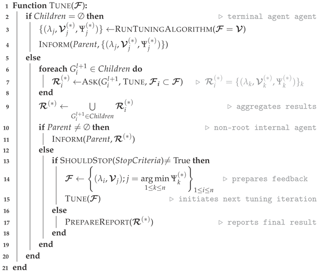 |
The details of the tuning function that each terminal agent runs in line 3 of Algorithm 2 to tune a single hyperparameter are presented in Algorithm 3. As its input, this function receives a coordinate that agent will use as its starting point in the searching process. The received argument, together with b additional coordinates that the agent generates randomly, are stored in the set of candidate . Accordingly, and refer to the c-th coordinate in the set and the value assigned to the hyperparameter of that coordinate, respectively. Moreover, please recall from Section 2.1 that b denotes the evaluation budget of a terminal agent. The terminal agents in the proposed method employ slot-based uniform random sampling to explore the search space. Formally, let be a set of real values that each agent utilizes for each hyperparameter to control the size of slots in any iteration. Similarly, let specify the coordinate of the position that an agent starts its searching operation in any iteration. To sample b random values in the domain of any arbitrary hyperparameter , the agent will generate one uniform random value in range
and random values in by splitting it into slots and choosing one uniform random value in each slot (lines 6 and 8 of the algorithm). The generation of the uniform random values is achieved by calling the function UniformRand(). This function divides range into equal-sized slots and returns the uniform random value generated in the -th slot. As it can be seen in line 12 of the algorithm, the agent employs the same function to generate one and only one value per each element in its subsidiary objective hyperparameter set .
The slot width parameter set is used to control the exploration behavior of the agent around the starting coordinates in the search space. For instance, for any arbitrary hyperparameter , very small values of emphasize generating candidates in the close vicinity of the starting position. Moreover, larger values of decrease the chance that the generated candidate will be close to the starting position. In the proposed method, the agents adjust adaptively. To put it formally, each agent starts the tuning process with the pre-specified value set , and assuming that denotes the best candidate that the agent has found in the previous iteration, the width parameter set in iteration i is updated as follows:
where denotes the scaling changes to apply to the width parameters, and ⊙ denotes the element-wise multiplication operator. As the paper discusses in Section 3, despite the generic definitions provided here for futuristic extensions, using the same scaling value for all primary hyperparameters has led to satisfactory results in our experiments.
| Algorithm 3: A terminal agent’s randomized tuning process. |
 |
To better understand the suggested collaborative randomized tuning process of agents, an illustrative example is depicted in Figure 2. In this figure, each agent is represented by a different color, and the best candidate that each agent finds at the end of each iteration is shown by a filled shape. Moreover, we have assumed that the value of the loss function becomes smaller as we move inwards in the depicted contour lines, and to prevent any exploration in the domain of the subsidiary hyperparameters, we have set and for agents and , respectively, assuming that the domain size of each hyperparameter is 1 and . In Iteration 1, both agents start at the top right corner of the search space and are able to find candidates that yield lower loss function values than the starting coordinate. For iteration 2, the starting coordinate of each agent is set to the coordinate of the best candidate found by all agents in the previous iteration. As the best candidate was found by agent , we only see the change in the searching direction of the red agent, i.e., . The winner agent at the end of this iteration is agent ; hence, we do not see any change to its searching direction in iteration 3. Please note that the four circles for agent in the last depicted iteration is because it shows the starting coordinate, which happens to remain the best candidate in this iteration. It is also worth emphasizing that the starting coordinates are not evaluated again by the agents, as they have already been accompanied by their corresponding response values from the previous iterations.
3. Results and Discussion
This section dissects the performance of the proposed method in more detail. It begins with the computational complexity of the technique and then provides empirical results on both machine learning and general function optimization tasks.
3.1. Computational Complexity
Forming the hierarchical structure and conducting the collaborative searching process are the two major stages of the proposed method and these stages need to be conducted in sequence. The rest of this section investigates the complexity of each step separately and in relation to one another.
Regarding the structural formation phase of the suggested method, the shape of the hierarchy depends on the maximum number of connections that each agent can handle; the fewer the number of manageable concurrent connections, the deeper the resulting hierarchy. Using the same notations presented in Section 2.1 and assuming the same for all agents, the depth of the formed hierarchy is . Thanks to the distributed nature of the formation algorithm and the concurrent execution of the agents, the worst-case time complexity of the first stage will be . With the same assumption, it can be easily shown that the resulting hierarchical structure is a complete tree. Hence, denoting the total number of agents in the system by , this quantity would be:
With that said, the space complexity for the first phase of the proposed technique would be . It is worth noting that among all created agents, only terminal agents would require dedicated computational resources as they are completing the actual searching and optimization process, and the remaining can all be hosted and managed together.
The procedures in each round of the second phase of the suggested method can be broken down into two main components: (i) transmitting the start coordinates from the root of the hierarchy to the terminal agents, transmitting the results back to the root, and preparing the feedback; and (ii) conducting the actual searching process by the terminal agents to locate a local optimum. The worst-case time complexity of preparing the feedback based on the algorithms that were discussed in Section 2 would be , which is because it finds the best candidate among all returned results. In addition, due to the concurrency of the agents, the first component is only processed at the height of the built structure. Therefore, the time complexity of component (i) would be . The complexity of the second component, moreover, depends on both the budget of the agent, i.e., b, and the complexity of building and evaluating response function . Let denote the time complexity of a single evaluation. As a terminal agent makes a b number of such evaluations to choose its candidate optima, the time complexity for the agent would be . As all agents work in parallel, the complexity of a single iteration at the terminal agents would be , leading to the overall time complexity of . In machine learning problems, we often have . Therefore, if denotes the number of iterations until the second phase of the tuning method stops, the complexity of the second stage would be . The space complexity of the second phase of the tuning method depends on the way that each agent is implementing the main functionalities, such as the learning algorithms they represent, transmitting the coordinates, and providing feedback. Except for the ML algorithms, all internal functionalities of each agent can be implemented using space. Moreover, we have agents in the system, which leads to a total space complexity of for non-ML tasks. Let denote the worst-case space complexity of a machine learning algorithm that we are tuning. The total space complexity of the second phase of the proposed tuning method would be . Similar to the time complexity, in machine learning, we often have , which makes the total space complexity of the second phase . Please note that we have factored out the budgets of the agents and the number of iterations because we did not store the history between different evaluations and iterations.
Considering both stages of the proposed technique and due to the fact that they are conducted in sequence, the time complexity of the entire steps in an ML hyperparameter tuning problem, from structure formation to completing the searching operations, would be . Similarly, the space complexity would be .
3.2. Empirical Results
This section presents the empirical results of employing the proposed agent-based randomized searching algorithm and discusses the improvements resulting from the suggested inter-agent collaborations. Hyperparameter tuning in machine learning is basically a back-box optimization problem, and hence, to enrich our empirical discussions, this section also includes results from multiple multi-dimensional optimization problems.
The performance metrics used for the experiments are based on those that are commonly used by the ML and optimization communities. Additionally, we analyze the behavior of the suggested methodology based on its own design parameter values, such as budget, width, etc. The methods that have been chosen for the sake of comparison are the standard random search and the Latin hypercube search methods [1] that are commonly used in practice. Our choices are based on the fact that not only are these methods embarrassingly parallel and among the top choices to be considered in distributed scenarios, but they are also used as the core optimization mechanisms of the terminal agents in the suggested method, and hence can better present the impact of the inter-agent collaborations. In its generic format, as emphasized in [20], one can easily employ alternative searching methods or diversify them at the terminal level, as needed.
Throughout the experiments, each terminal agent runs on a separate process, and to make the comparisons fair, we keep the number of model/function evaluations fixed among all of the experimented methods. To put it in more detail, for a budget value of b for each of terminal agents and number of iterations, the proposed method will evaluate the search space in coordinates. We use the same number of independent agents for the compared random-based methodologies and, keeping the evaluation budgets of the agents fixed—the budgets are assumed to be enforced by the computational limitations of devices or processes running the agents—we repeat those methods times and report the best performance among all agents’ repetition histories as their final result.
The experiments assess the performance of the proposed method in comparison to the other random-based techniques in four categories: (1) iteration-based assessment, which checks the performance of the methods for a particular iteration threshold. In this category, all other parameters, such as budget, connection number, etc., are kept fixed; (2) budget-based assessment, which examines the performance under various evaluation budgets for the terminal agents. It is assumed that all agents have the same budget; (3) width-based assessment, which checks how the proposed method performs for various exploration criteria specified by the slot width parameter; and finally, (4) connection-based evaluation, which inspects the effect of the parallel connection numbers that the internal agents can handle. In other words, this evaluation checks if the proposed method is sensitive to the way that the hyperparameter or decision variables are split during the hierarchy formation phase. All implementations use Python 3.9 and the scikit-learn library [26], and the results reported in all experiments are based on 50 different trials.
For the ML hyperparameter tuning experiments, we have dissected the behavior of the proposed algorithm in two classifications and two regression problems. The details of such problems, including the hyperparameters that are tuned and the used datasets are presented in Table 1. In all of the ML experiments, we have used five-fold cross-validation as the model evaluation method. The results obtained for the classification and regression problems are plotted in Figure 3 and Figure 4, respectively. Please note that there are numerous ML algorithms that can be used to evaluate our approach. Our selected algorithms are representative of different types of classifiers/regressors, including linear and non-linear models with different regularization methods, and we found them widely used in hyperparameter tuning literature based on their performance sensitivity to the choice of hyperparameter values. We also experienced this empirically during our evaluations of some other ML algorithms. We found that all of the compared models converged to a local optimum point quickly, potentially due to the geometry of their response functions, which would not demonstrate the improvements of our model. By comparing the performance of the presented methods on these models, we hope to draw more general conclusions about the effectiveness of the methods in various settings.
For the iterations plot in the first column plots of Figure 3 and Figure 4, we fixed the parameters of the proposed method for all agents as follows: . As can be seen, when the proposed method is allowed to run for more iterations, it yields better performance, and its superiority against the other two random-based methods is evident. Comparing the relative performance improvements resulting from the proposed method in the presented ML tasks, it can be seen that as the search space of the agents and the number of hyperparameters needed to be tuned increased, the proposed collaborative method achieved a higher improvement. For the Stochastic Gradient Descent (SGD) classifier, for instance, the objective hyperparameter set comprises six members with continuous domain spaces, and the number of improvements that have been made after 10 iterations is much higher, about 17%, than in the other experiments with three to four hyperparameters and mixed continuous and discrete domain spaces.

Table 1.
The details of the machine learning algorithms and the datasets used for hyperparameter tuning experiments.
Table 1.
The details of the machine learning algorithms and the datasets used for hyperparameter tuning experiments.
| ML Algorithm | Dataset | Performance Metric | |
|---|---|---|---|
| C-Support Vector Classification (SVC) [26,27] | 1 | artificial (100,20) † | accuracy |
| Stochastic Gradient Descent (SGD) Classifier [26] | 2 | artificial (500,20) † | accuracy |
| Passive Aggressive Regressor [26,28] | 3 | artificial (300,100) ‡ | mean squared error |
| Elastic Net Regressor [26,29] | 4 | artificial (300,100) ‡ | mean squared error |
1 c∼∼. 2 ∼∼∼∼∼∼. 3 c∼∼∼∼. 4 ∼∼∼. † An artificially generated binary classification dataset using scikit-learn’s make_classification function [30]. The first number represents the number of samples and the second figure is the number of features. ‡ An artificially generated regression dataset using scikit-learn’s make_regression function [30]. The first number represents the number of samples and the second figure is the number of features.
The second column of Figure 3 and Figure 4 illustrate how the performance of the proposed technique changes when we increase the evaluation budgets of the terminal agents. For this set of experiments, we set the parameter values of our method as follows: . By increasing the budget value, the performance of the suggested approach per se improves. However, the rate of improvement slows down for higher budget values, and comparing it against the performance of the other two random-based searching methods, the improvement is significant for lower budget values. In other words, the proposed tuning method surpasses the other two methods when the agents have limited searching resources. This makes our method a good candidate for tuning the hyperparameters of deep learning approaches with expensive model evaluations.
The behavior of the suggested method under various exploration parameter values can be seen in column 3 of Figure 3 and Figure 4. The values on the x-axis of the plots are used to set the initial value for the slot width parameter of all agents using . Based on this configuration, higher values of yield lower values of , and as a result, there is more exploitation around the starting coordinates. The other parameters of the method are configured as follows: . Recall from Section 2 that the exploration parameter is used by an agent for the dimensions that it does not represent. Based on the results obtained from various tasks, choosing a proper value for this parameter depends on the characteristics of the response function. Having said that, the behavior for a particular task remains almost consistent. Hence, trying one small and one large value for this parameter in a specific problem will reveal its sensitivity and help choose an appropriate value for it.
Finally, the last set of experiments investigates the impact of the number of parallel connections that the internal agents can manage, i.e., c, on the performance of the suggested method. The results of this study are plotted in the last column of Figure 3 and Figure 4. The difference in the number of data points in each plot is because of the difference in the size of the hyperparameters that we tune for each task. The values of the parameters that we kept fixed for this set of experiments are as follows: . As can be seen from the illustrated results, the proposed method is not very sensitive to the value that we choose or that is enforced by the system for parameter c. This parameter plays a critical role in the shape of the hierarchy that is distributedly formed in phase 1 of the suggested approach; therefore, one can opt to choose a value that fits with the connection or computational resources that are available without sacrificing performance very much.
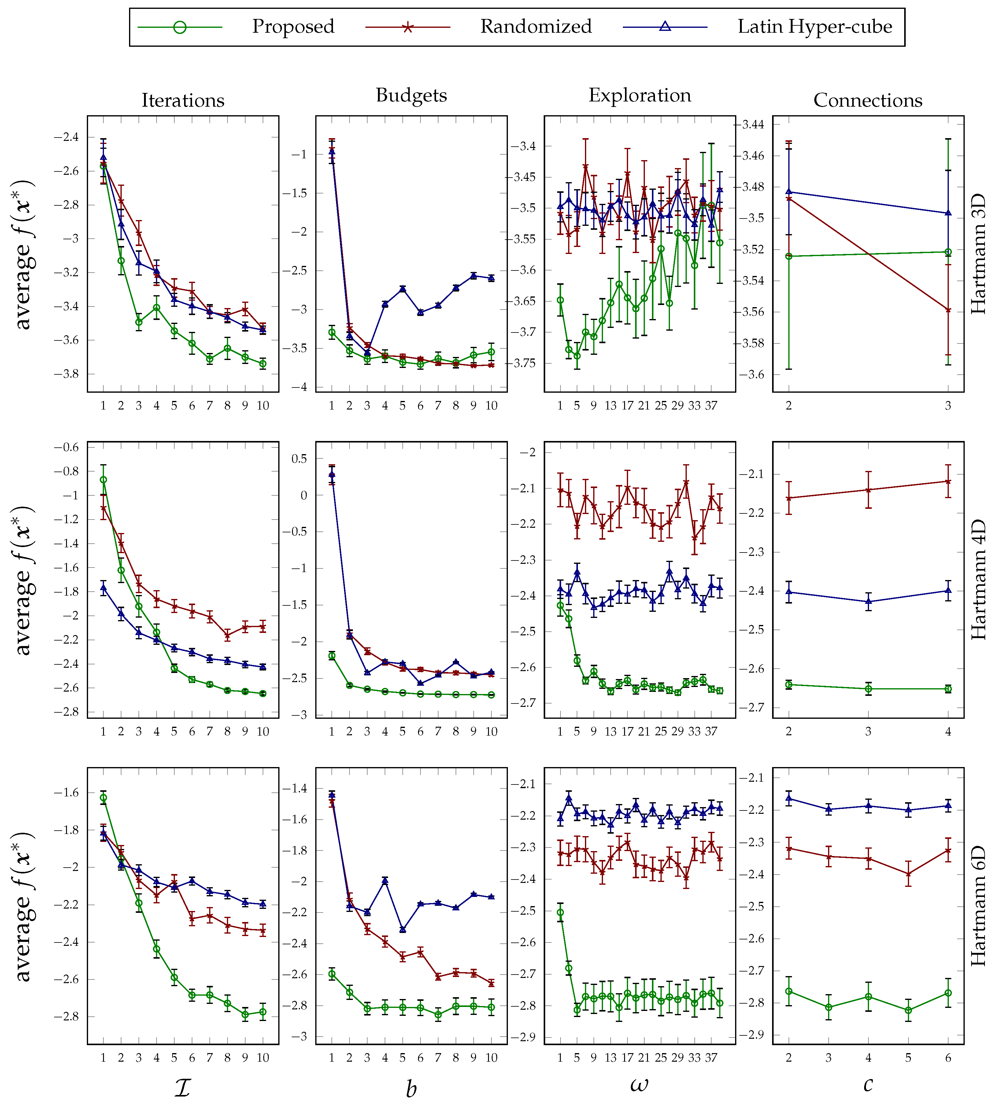
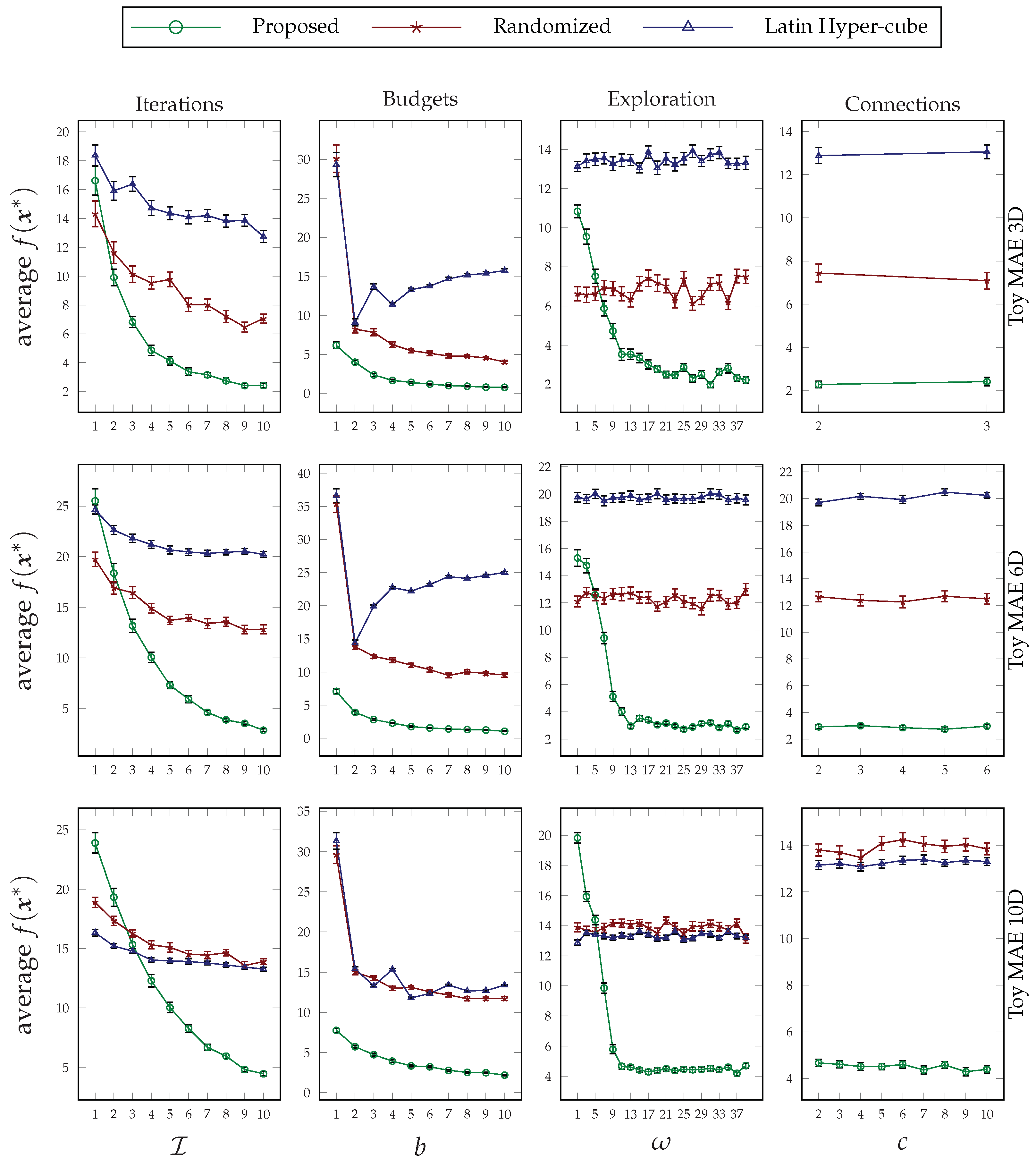
As stated before, we have also studied the suggested technique for the black-box optimization problem to see how it performs in finding the optima of various convex and non-convex functions. These experiments also help us to closely check the relative performance improvements in higher dimensions. We have chosen three non-convex benchmark optimization functions and a convex toy function, the details of which are presented in Table 2. For each function, we run the experiments in three different dimension sizes, and the goal of the optimization is to find the global minimum. Very similar to the settings that we discussed for ML hyperparameter tuning, whenever we mean to fix the value of each parameter value in different experiment sets, we use the following parameter values: .
Table 2.
The details of the multi-dimensional functions used for black-box optimization experiments.
Table 2.
The details of the multi-dimensional functions used for black-box optimization experiments.
| Function | Domain | ||
|---|---|---|---|
| Hartmann, 3D, 4D, 6D [31] | 3D:−3.86278, 4D:−3.135474, 6D:−3.32237 | ||
| Rastrigin, 3D, 6D, 10D [32] | 3D:0, 6D:0, 10D:0 | ||
| Styblinski–Tang, 3D, 6D, 10D [33] | 3D:−117.4979, 6D:−234.9959, 10D:391.6599 | ||
| Mean Average Error, 3D, 6D, 10D † | 3D:0,6D:0, 10D:0 ‡ |
† This is a toy multi-dimensional MAE function that is defined as , where denotes a ground truth vector that is generated randomly in the domain space for each experiment. ‡ This is a convex function and the coordinate of its minimum value depends on the ground truth vector that is generated, i.e., when .
The plots are grouped by functions and can be found in Figure 5, Figure 6, Figure 7 and Figure 8. The conclusion that was drawn concerning the behavior of the proposed approach under different values of its design parameters applies to these optimization experiments as well. That is, the more the proposed method runs, the better performance it achieves; its superiority on low budget values is clear; its sensitivity to exploration parameter values is consistent; and the way that the decision variables are broken down during the formation of the hierarchy does not affect the performance very much. Furthermore, as can be seen in each group figure, the proposed algorithm yields a better minimum point in comparison to the other two random-based methods when the dimensionality of a function increases.
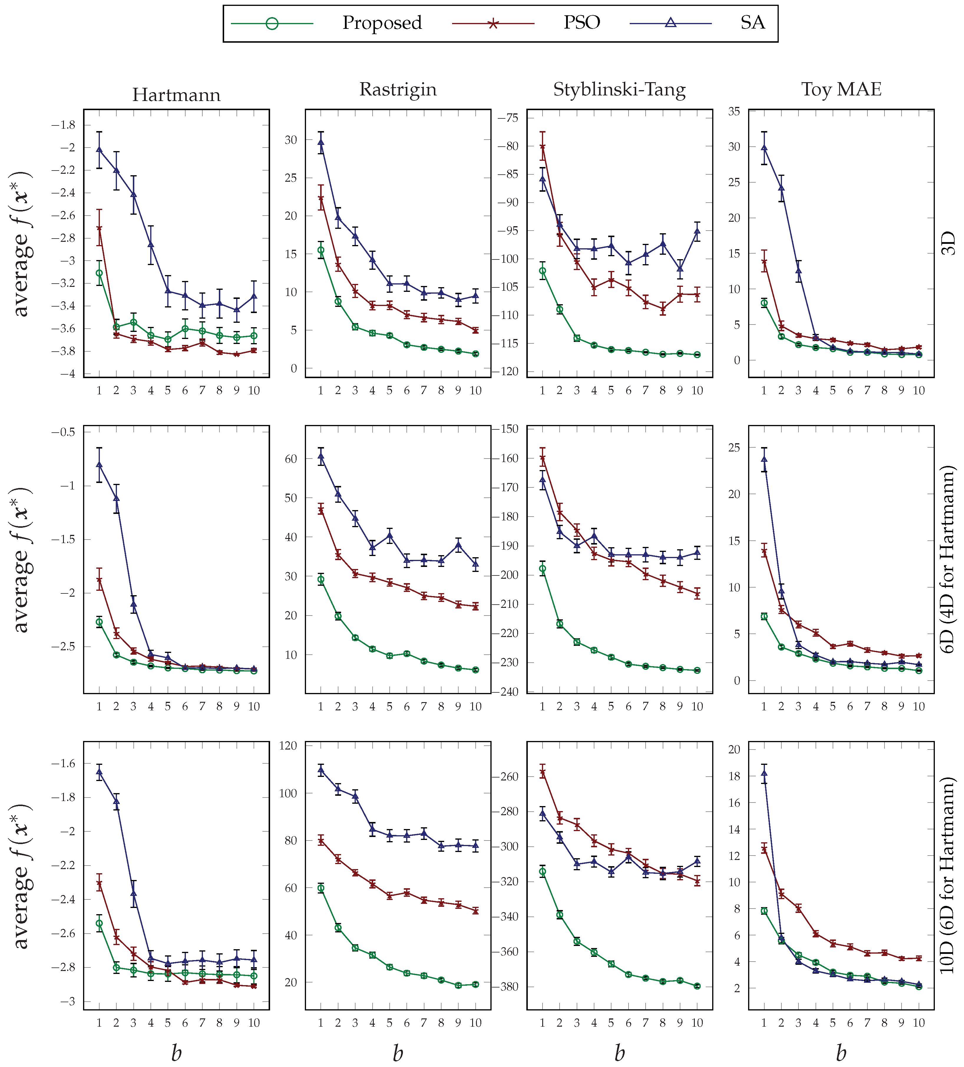
Disregarding its multi-agent formulation, autonomy, and inter-agent collaborations, the proposed method shares similarities with heuristic and population-based black-box optimization approaches. We believe that even with such a viewpoint, our method can be more applicable due to its simple architecture, low number of hyperparameters, its innate distribution, and because it requires less domain knowledge. Figure 9 and Figure 10 provide a comparison between the performance of our agent-based method and the ones of particle swarm optimization (PSO) [34] and simulated annealing (SA) [35]. Please note that these comparisons are not to prove our method’s superiority over population-based and/or heuristic methods, but to give a glimpse into some additional behaviors and the potentiality of the agent-based solution. In its current immature condition, we do not doubt that our immature approach will most probably be outperformed by the many mature heuristic methods available.
For the PSO algorithm, we have employed the standard version and set its hyperparameter values as and . As for the SA algorithm, we have used Kirkpatrick’s method [35] to define the accepting probabilities with and the geometric process for the annealing schedule, i.e., with . Please note that our choices for the aforementioned values are based on multiple trials and errors and the general practical suggestions found in the literature. Finally, the values that we have utilized for our agent-based solution are as follows: and , whenever they are assumed fixed. Please note that these values are the same as the ones we applied in the previous set of analyses, and we have not conducted any optimization to choose the best possible values.
Due to the different underlying principles used in each of these algorithms, providing an absolutely fair comparison would not be possible. For instance, in our method, the number of agents is fixed, and each agent has an evaluation budget. In the PSO algorithm, however, the population size is a hyperparameter, and each particle makes a single evaluation. The SA, moreover, is a single-agent, centralized approach with one evaluation in each of its iterations. To the best of our ability, in this empirical comparison, we have tried to keep the total number of evaluations fixed among all experiments. Strictly speaking, we set the same number of iterations, i.e., , in the PSO but set its population size to . Similarly, in the SA, we set the number of iterations to .
The results presented in Figure 9 show how each different method behaves under different numbers of iterations in each of the benchmark problems. As can be seen, in most benchmarks, the proposed method has outperformed both PSO and SA in higher iteration numbers. Recalling the true optimal function values from Table 2, the tied or close conditions among all methods happen near the global optima, which we believe can be improved through an adaptive exploitation method. Furthermore, due to the relatively higher improvements in the Rastrigin and Styblinski–Tang functions and the fact that these two functions are composed of several local optima, we can conclude that our proposed method has better capability to escape those local positions.
The results exhibited in Figure 10 show the behavior of the tested optimization algorithms under various budget restrictions. In this set of experiments, we have fixed the number of iterations to , and the results show a promising success of our method in outperforming the other two in most problems. Similar to the rationale provided above, the amount of improvement in Rastrigin and Styblinski–Tang functions is evident. Moreover, our method also shines when we have a low budget for the number of evaluations in each iteration. In other words, it can be a good candidate for optimizing expensive-to-evaluate problems or its use in computationally limited devices.
Regarding the computational time, we extend our analysis of the time complexity of the proposed methods in the previous section to the compared random-based methods. Let , and denote the evaluation budget of each agent, the number of iterations, and the total number of hyperparameter/decision variables to be optimized, respectively. As we have compared the methods under fair conditions, i.e., giving each agent the opportunity to run its randomized algorithm for times, and since we have assumed that all agents run independently in parallel, the time complexity of both “randomized” and “Latin hypercube” methods would be , where denotes the complexity of the underlying ML model or function evaluation. Recall from the previous section that the time complexity of the proposed method is due to its initial structure formation phase and the vertical communication of non-terminal agents. In other words, our proposed approach requires additional computational time in the worst case. The worst case occurs when the computational time complexity of the evaluation of the objective function or the ML model, i.e., , is low. In almost all ML tasks however, we have , hence the time difference is negligible. It is worth emphasizing that this comparison is based on the assumption of a fair comparison and parallel execution of the budgeted agents. It is clear that any changes applied to the benefit of a particular method will definitely change the requirements. For instance, if we limit the number of evaluations in randomized methods, they will require less time to find a local minimum; however, the result will be of lower quality. Regarding the tested heuristic methods, as we have kept the number of evaluations fixed and due to using a similar amount of work internally, we expect a computational complexity similar to our approach for them.
It is worth reiterating that the contribution of this paper is not to compete with the state-of-the-art algorithms in function optimization, but to propose a distributed tuning/optimization approach that can be deployed on a set of distributed and networked devices. The discussed analytical and empirical results not only demonstrated the behavior and impact of the design parameters that we have used in our approach, but also suggested the way that they can be adjusted for different needs. We believe the contribution of this paper can be significantly improved with more sophisticated and carefully chosen tuning strategies and corresponding configurations.
4. Conclusions
This paper presented an agent-based collaborative random search method that can be used for machine learning hyper-parameter tuning and black-box optimization problems. The approach employs two types of agents during the tuning/optimization process: the internal and terminal agents that are responsible for facilitating collaborations and tuning individual decision variables, respectively. Such agents and the interaction network between them are created during the hierarchy formation phase and remain the same for the entire runtime of the suggested method. Thanks to the modular and distributed nature of the approach and its procedures, it can be easily deployed on a network of devices with various computational capabilities. Furthermore, the design parameters used in this technique enable each individual agent to customize its own searching process and behavior independent from its peers in the hierarchy, allowing for diversity in both algorithmic and deployment levels.
The paper dissected the proposed model from different aspects and provided some tips on handling its behavior for various applications. According to the analytical discussions, our approach requires slightly more computational and storage resources than the traditional and Latin hypercube randomized search methods that are commonly used for both hyper-parameter tuning and black-box optimization problems. However, this results in significant performance improvements, especially in computationally restricted circumstances with higher numbers of decision variables. This conclusion was verified in both machine learning model tuning tasks and general multi-dimensional function optimization problems. Furthermore, the empirical results on two widely used heuristic methods, namely PSO and SA, showed that our method exhibits better exploration and potential for escaping local optima while using limited computational resources.
The presented work can be further extended both technically and empirically. As was discussed throughout this paper, we kept the searching strategies and the way the design parameters are configured as simple as possible so we could reach a better understanding of the effectiveness of the collaborations and searching space divisions. A few potential extensions in this direction include: the utilization of diverse searching methods, hence the possession of a heterogeneous multi-agent system at the terminal level; the split of the searching space that is not based on the dimensions, but rather on the range of the values that decision variables in each dimension can have; employment of more sophisticated collaboration techniques; and the use of a learning-based approach to dynamically adapt the values of the design parameters during the runtime of the method. Empirically, the presented research can be extended by completing an in-depth comparison with population-based methods and applying our method to expensive machine learning tasks, such as tuning deep learning models with a large number of hyper-parameters. We are currently working on some of these studies and suggest them as future work.
Author Contributions
Methodology, A.E.; validation, Z.G.; investigation, A.E. and Z.G.; writing—original draft, A.E.; writing—review and editing, Z.G.; visualization, A.E.; supervision, E.T.M. All authors have read and agreed to the published version of the manuscript.
Funding
This research received no external funding.
Conflicts of Interest
The authors declare no conflict of interest.
References
- Bergstra, J.; Bengio, Y. Random search for hyper-parameter optimization. J. Mach. Learn. Res. 2012, 13, 281–305. [Google Scholar]
- Kohavi, R.; John, G.H. Automatic parameter selection by minimizing estimated error. In Machine Learning Proceedings 1995; Elsevier: Amsterdam, The Netherlands, 1995; pp. 304–312. [Google Scholar]
- Bischl, B.; Mersmann, O.; Trautmann, H.; Weihs, C. Resampling Methods for Meta-Model Validation with Recommendations for Evolutionary Computation. Evol. Comput. 2012, 20, 249–275. [Google Scholar] [CrossRef] [PubMed]
- Montgomery, D.C. Design and Analysis of Experiments; John Wiley & Sons: Hoboken, NJ, USA, 2017. [Google Scholar]
- John, G.H. Cross-Validated C4.5: Using Error Estimation for Automatic Parameter Selection; Technical Report; Stanford University: Stanford, CA, USA, 1994. [Google Scholar]
- Močkus, J. On Bayesian methods for seeking the extremum. In Proceedings of the Optimization Techniques IFIP Technical Conference, Novosibirsk, Russia, 1–7 July 1974; Springer: Berlin/Heidelberg, Germany, 1975; pp. 400–404. [Google Scholar]
- Mockus, J. Bayesian Approach to Global Optimization: Theory and Applications; Springer Science & Business Media: Berlin/Heidelberg, Germany, 2012; Volume 37. [Google Scholar]
- Feurer, M.; Hutter, F. Hyperparameter optimization. In Automated Machine Learning; Springer: Cham, Switzerland, 2019; pp. 3–33. [Google Scholar]
- Simon, D. Evolutionary Optimization Algorithms; John Wiley & Sons: Hoboken, NJ, USA, 2013. [Google Scholar]
- Alibrahim, H.; Ludwig, S.A. Hyperparameter Optimization: Comparing Genetic Algorithm against Grid Search and Bayesian Optimization. In Proceedings of the 2021 IEEE Congress on Evolutionary Computation (CEC), Kraków, Poland, 28 June–1 July 2021; pp. 1551–1559. [Google Scholar]
- Bellman, R.E. Adaptive Control Processes; Princeton University Press: Princeton, NJ, USA, 1961. [Google Scholar]
- Shahriari, B.; Swersky, K.; Wang, Z.; Adams, R.P.; De Freitas, N. Taking the human out of the loop: A review of Bayesian optimization. Proc. IEEE 2015, 104, 148–175. [Google Scholar] [CrossRef]
- Garcia-Barcos, J.; Martinez-Cantin, R. Fully Distributed Bayesian Optimization with Stochastic Policies. In Proceedings of the Twenty-Eighth International Joint Conference on Artificial Intelligence, Macao, China, 10–16 August 2019. [Google Scholar]
- Young, M.T.; Hinkle, J.D.; Kannan, R.; Ramanathan, A. Distributed Bayesian optimization of deep reinforcement learning algorithms. J. Parallel Distrib. Comput. 2020, 139, 43–52. [Google Scholar] [CrossRef]
- Frazier, P.I. A Tutorial on Bayesian Optimization. arXiv 2018, arXiv:1807.02811. [Google Scholar] [CrossRef]
- Friedrichs, F.; Igel, C. Evolutionary tuning of multiple SVM parameters. Neurocomputing 2005, 64, 107–117. [Google Scholar] [CrossRef]
- Loshchilov, I.; Hutter, F. CMA-ES for hyperparameter optimization of deep neural networks. arXiv 2016, arXiv:1604.07269. [Google Scholar]
- Ryzko, D. Modern Big Data Architectures: A Multi-Agent Systems Perspective; John Wiley & Sons: Hoboken, NJ, USA, 2020. [Google Scholar]
- Esmaeili, A.; Gallagher, J.C.; Springer, J.A.; Matson, E.T. HAMLET: A Hierarchical Agent-Based Machine Learning Platform. ACM Trans. Auton. Adapt. Syst. 2022, 16, 1–46. [Google Scholar] [CrossRef]
- Esmaeili, A.; Ghorrati, Z.; Matson, E.T. Hierarchical Collaborative Hyper-Parameter Tuning. In Proceedings of the Advances in Practical Applications of Agents, Multi-Agent Systems, and Complex Systems Simulation. The PAAMS Collection, L’Aquila, Italy, 13–15 July 2022; Springer International Publishing: Cham, Switzerland, 2022; pp. 127–139. [Google Scholar]
- Bardenet, R.; Brendel, M.; Kégl, B.; Sebag, M. Collaborative hyperparameter tuning. In Proceedings of the International Conference on Machine Learning, PMLR, Atlanta, GA, USA, 17–19 June 2013; pp. 199–207. [Google Scholar]
- Swearingen, T.; Drevo, W.; Cyphers, B.; Cuesta-Infante, A.; Ross, A.; Veeramachaneni, K. ATM: A distributed, collaborative, scalable system for automated machine learning. In Proceedings of the 2017 IEEE International Conference on Big Data (Big Data), Boston, MA, USA, 11–14 December 2017; pp. 151–162. [Google Scholar]
- Koch, P.; Golovidov, O.; Gardner, S.; Wujek, B.; Griffin, J.; Xu, Y. Autotune: A derivative-free optimization framework for hyperparameter tuning. In Proceedings of the 24th ACM SIGKDD International Conference on Knowledge Discovery & Data Mining, London, UK, 19–23 August 2018; pp. 443–452. [Google Scholar]
- Iranfar, A.; Zapater, M.; Atienza, D. Multi-agent reinforcement learning for hyperparameter optimization of convolutional neural networks. IEEE Trans. Comput.-Aided Des. Integr. Circuits Syst. 2021, 41, 1034–1047. [Google Scholar] [CrossRef]
- Parker-Holder, J.; Nguyen, V.; Roberts, S.J. Provably efficient online hyperparameter optimization with population-based bandits. Adv. Neural Inf. Process. Syst. 2020, 33, 17200–17211. [Google Scholar]
- Pedregosa, F.; Varoquaux, G.; Gramfort, A.; Michel, V.; Thirion, B.; Grisel, O.; Blondel, M.; Prettenhofer, P.; Weiss, R.; Dubourg, V.; et al. Scikit-learn: Machine Learning in Python. J. Mach. Learn. Res. 2011, 12, 2825–2830. [Google Scholar]
- Chang, C.C.; Lin, C.J. LIBSVM: A library for support vector machines. ACM Trans. Intell. Syst. Technol. (TIST) 2011, 2, 1–27. [Google Scholar] [CrossRef]
- Crammer, K.; Dekel, O.; Keshet, J.; Shalev-Shwartz, S.; Singer, Y. Online passive aggressive algorithms. J. Mach. Learn. Res. 2006, 7, 551–585. [Google Scholar]
- Friedman, J.; Hastie, T.; Tibshirani, R. Regularization paths for generalized linear models via coordinate descent. J. Stat. Softw. 2010, 33, 1. [Google Scholar] [CrossRef] [PubMed]
- Scikit-Learn API Reference. Available online: https://scikit-learn.org/stable/modules/classes.html (accessed on 24 November 2022).
- Jamil, M.; Yang, X.S. A literature survey of benchmark functions for global optimisation problems. Int. J. Math. Model. Numer. Optim. 2013, 4, 150. [Google Scholar] [CrossRef]
- Rudolph, G. Globale Optimierung Mit Parallelen Evolutionsstrategien. Ph.D. Thesis, Diplomarbeit, Universit at Dortmund, Fachbereich Informatik, Dortmund, Germany, 1990. [Google Scholar]
- Styblinski, M.; Tang, T.S. Experiments in nonconvex optimization: Stochastic approximation with function smoothing and simulated annealing. Neural Netw. 1990, 3, 467–483. [Google Scholar] [CrossRef]
- Kennedy, J.; Eberhart, R. Particle swarm optimization. In Proceedings of the ICNN’95-International Conference on Neural Networks, Perth, WA, Australia, 27 November–1 December 1995; Volume 4, pp. 1942–1948. [Google Scholar]
- Kirkpatrick, S.; Gelatt, C.D., Jr.; Vecchi, M.P. Optimization by simulated annealing. Science 1983, 220, 671–680. [Google Scholar] [CrossRef]
Figure 1.
Hierarchical structure built for , where the primary and complementary hyperparameters of each node are, respectively, highlighted in green and orange, and the labels are the indexes of .
Figure 1.
Hierarchical structure built for , where the primary and complementary hyperparameters of each node are, respectively, highlighted in green and orange, and the labels are the indexes of .
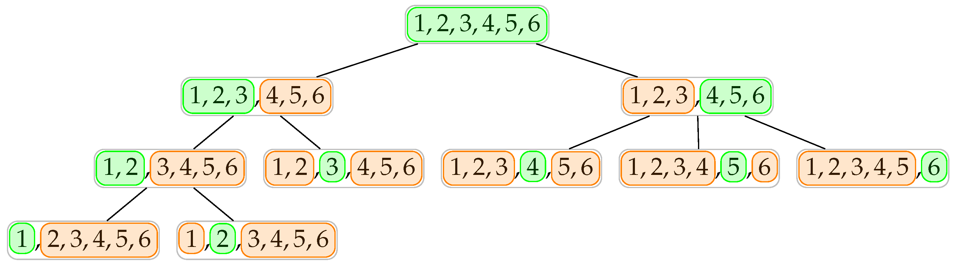
Figure 2.
A toy example demonstrating three iterations of running the proposed method for tuning two hyperparameters and using terminal agents and , respectively. It is assumed that for each agent, .
Figure 2.
A toy example demonstrating three iterations of running the proposed method for tuning two hyperparameters and using terminal agents and , respectively. It is assumed that for each agent, .
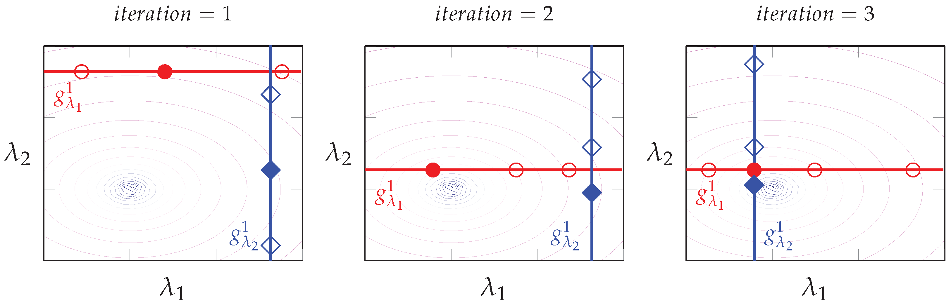
Figure 3.
Average performance of the C-support vector classification (SVC) (first row) and stochastic gradient descent (SGD) (second row) classifiers on two synthetic classification datasets based on the accuracy measure. The error bars in each plot are calculated based on the standard error.
Figure 3.
Average performance of the C-support vector classification (SVC) (first row) and stochastic gradient descent (SGD) (second row) classifiers on two synthetic classification datasets based on the accuracy measure. The error bars in each plot are calculated based on the standard error.
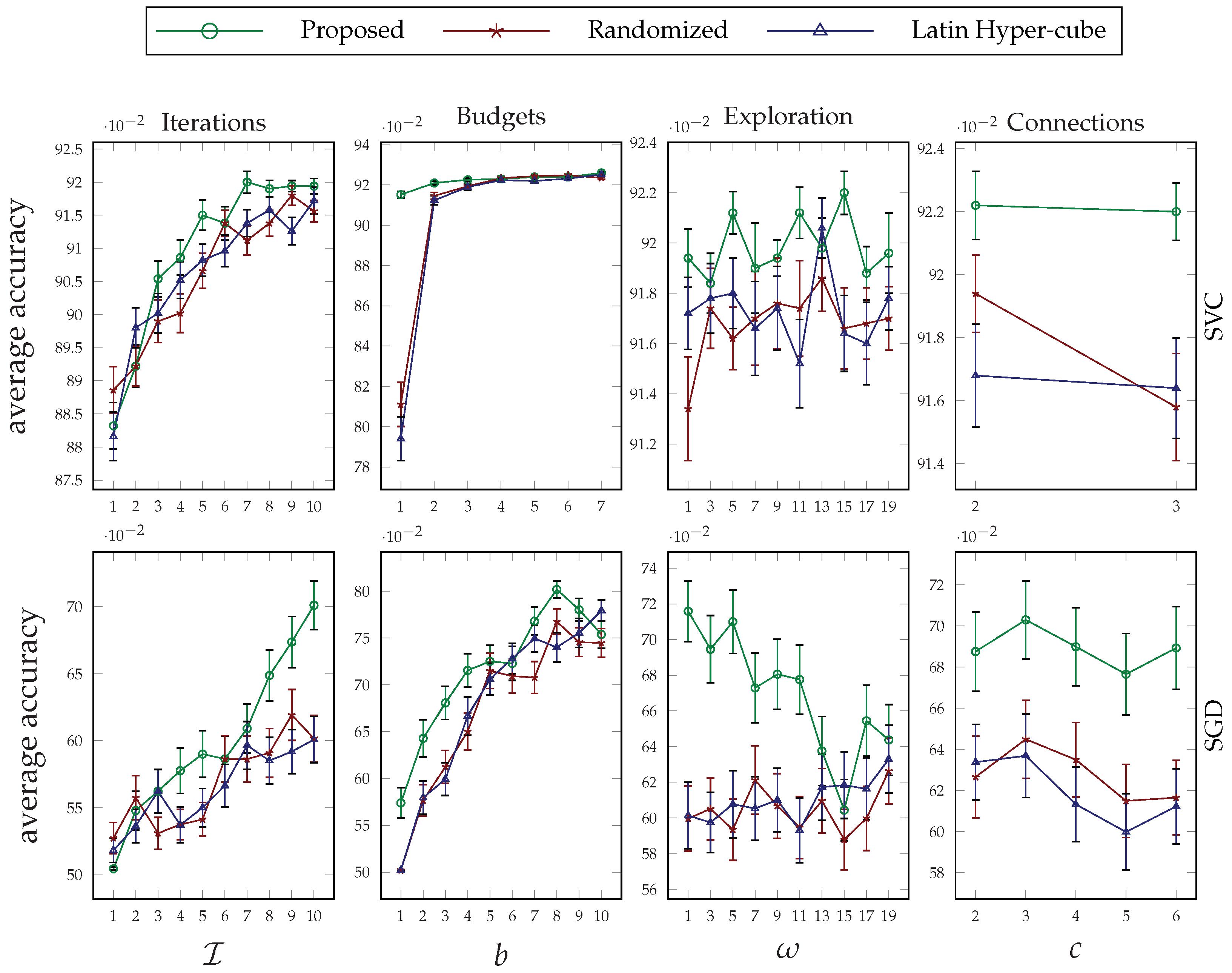
Figure 4.
Average performance of the passive aggressive (first row) and elastic net (second row) regression algorithms on two synthetic regression datasets based on the mean squared error (MSE) measure. The error bars in each plot are calculated based on the standard error.
Figure 4.
Average performance of the passive aggressive (first row) and elastic net (second row) regression algorithms on two synthetic regression datasets based on the mean squared error (MSE) measure. The error bars in each plot are calculated based on the standard error.
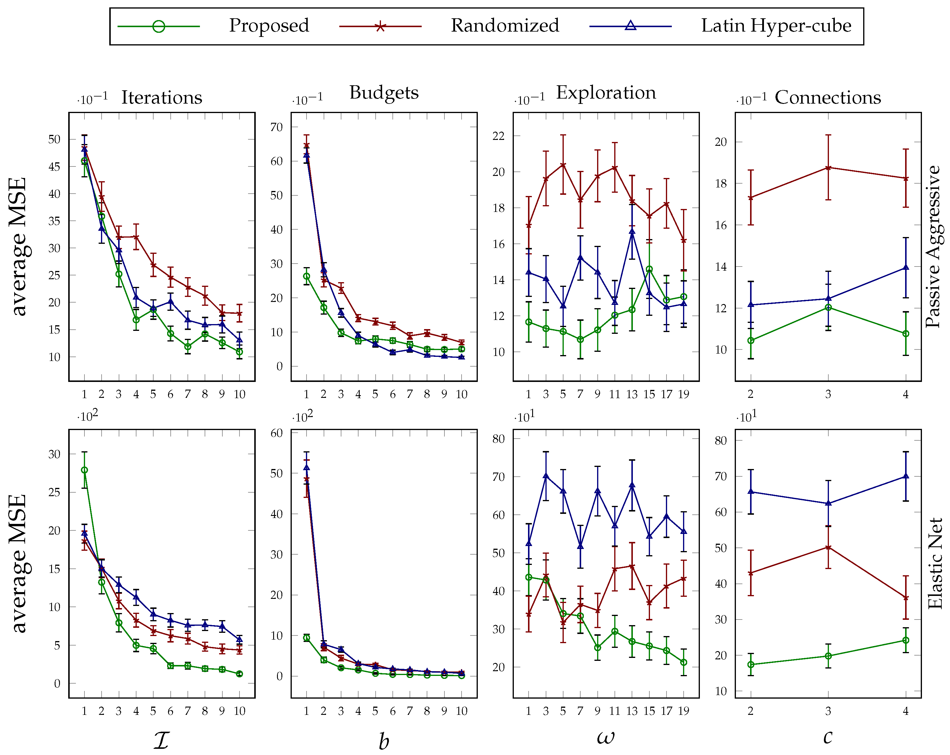
Figure 5.
Average values of the Hartmann function optimized under variable iterations, budgets, explorations, and connection thresholds. Each row of the figure pertains to a particular dimension size, and the error bars are calculated based on the standard error.
Figure 5.
Average values of the Hartmann function optimized under variable iterations, budgets, explorations, and connection thresholds. Each row of the figure pertains to a particular dimension size, and the error bars are calculated based on the standard error.

Figure 6.
Average values of the Rastrigin function optimized under variable iterations, budgets, explorations, and connection thresholds. Each row of the figure pertains to a particular dimension size, and the error bars are calculated based on the standard error.
Figure 6.
Average values of the Rastrigin function optimized under variable iterations, budgets, explorations, and connection thresholds. Each row of the figure pertains to a particular dimension size, and the error bars are calculated based on the standard error.
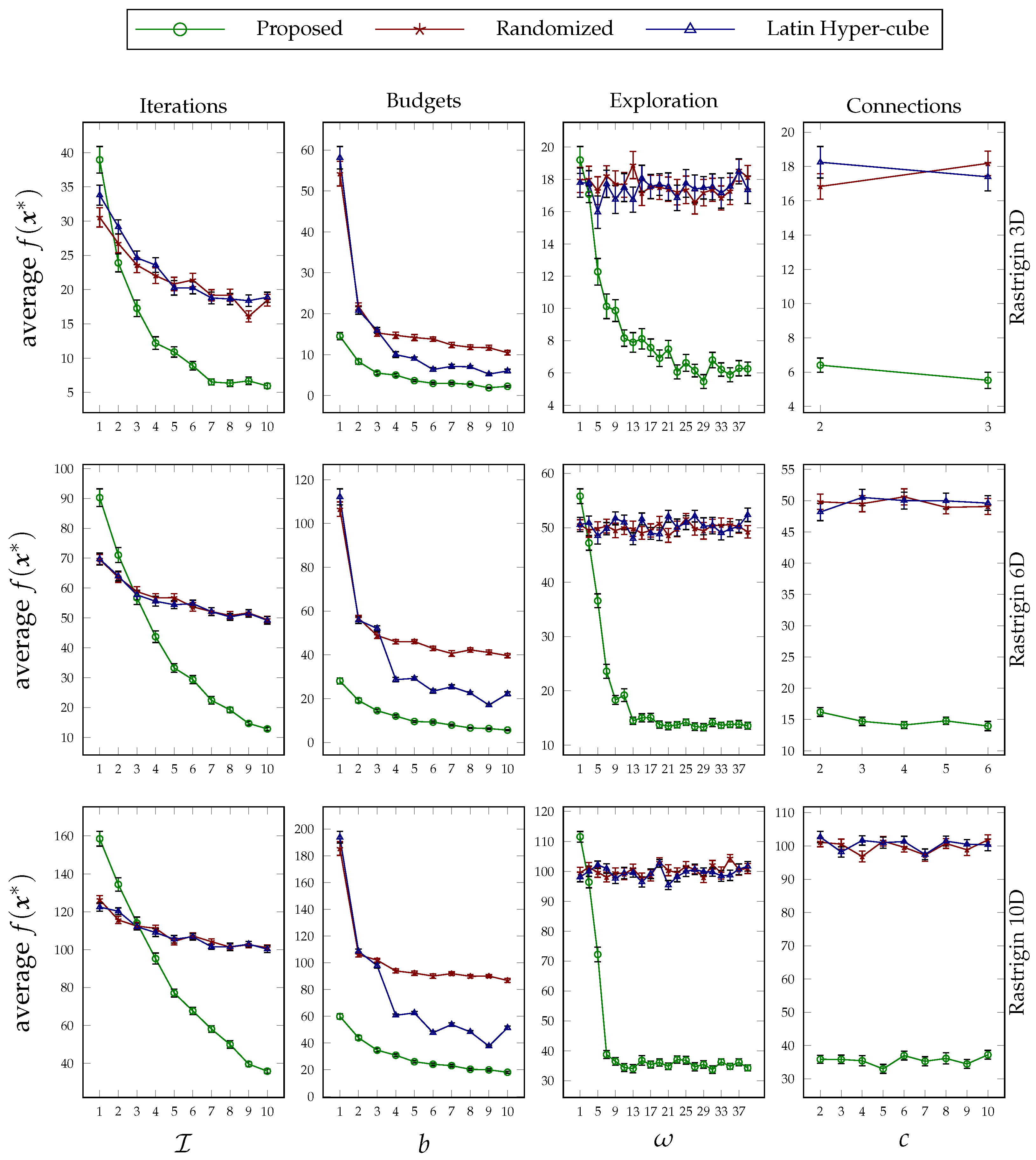
Figure 7.
Average values of the Styblinski–Tang function optimized under variable iterations, budgets, explorations, and connection thresholds. Each row of the figure pertains to a particular dimension size, and the error bars are calculated based on the standard error.
Figure 7.
Average values of the Styblinski–Tang function optimized under variable iterations, budgets, explorations, and connection thresholds. Each row of the figure pertains to a particular dimension size, and the error bars are calculated based on the standard error.
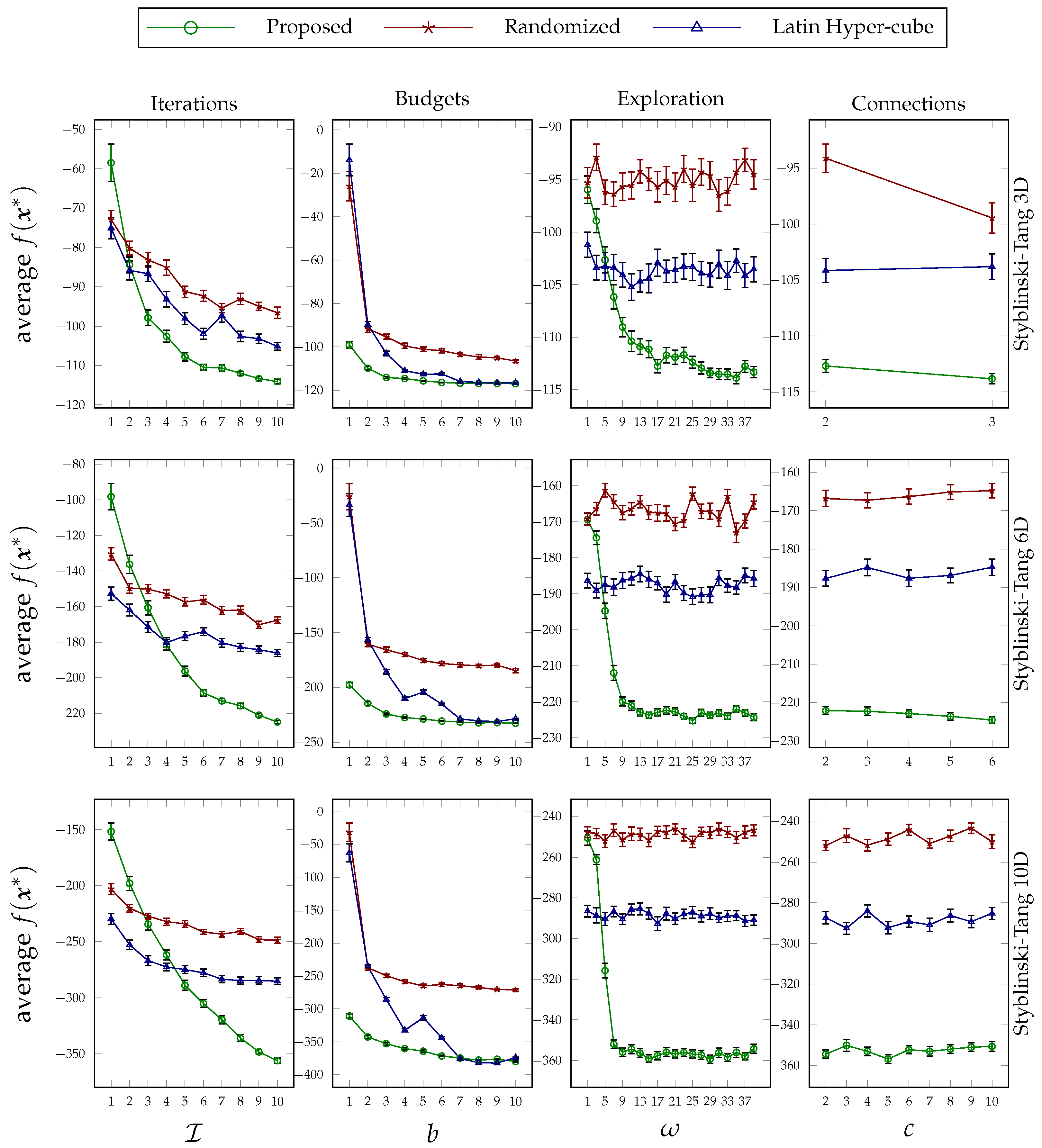
Figure 8.
Average values of the toy mean absolute error function optimized under variable iterations, budgets, explorations, and connection thresholds. Each row of the figure pertains to a particular dimension size, and the error bars are calculated based on the standard error.
Figure 8.
Average values of the toy mean absolute error function optimized under variable iterations, budgets, explorations, and connection thresholds. Each row of the figure pertains to a particular dimension size, and the error bars are calculated based on the standard error.

Figure 9.
Average function values of four objective functions optimized under a variable number of iterations. Each row of the figure pertains to a particular dimension size, and the error bars are calculated based on the standard error.
Figure 9.
Average function values of four objective functions optimized under a variable number of iterations. Each row of the figure pertains to a particular dimension size, and the error bars are calculated based on the standard error.
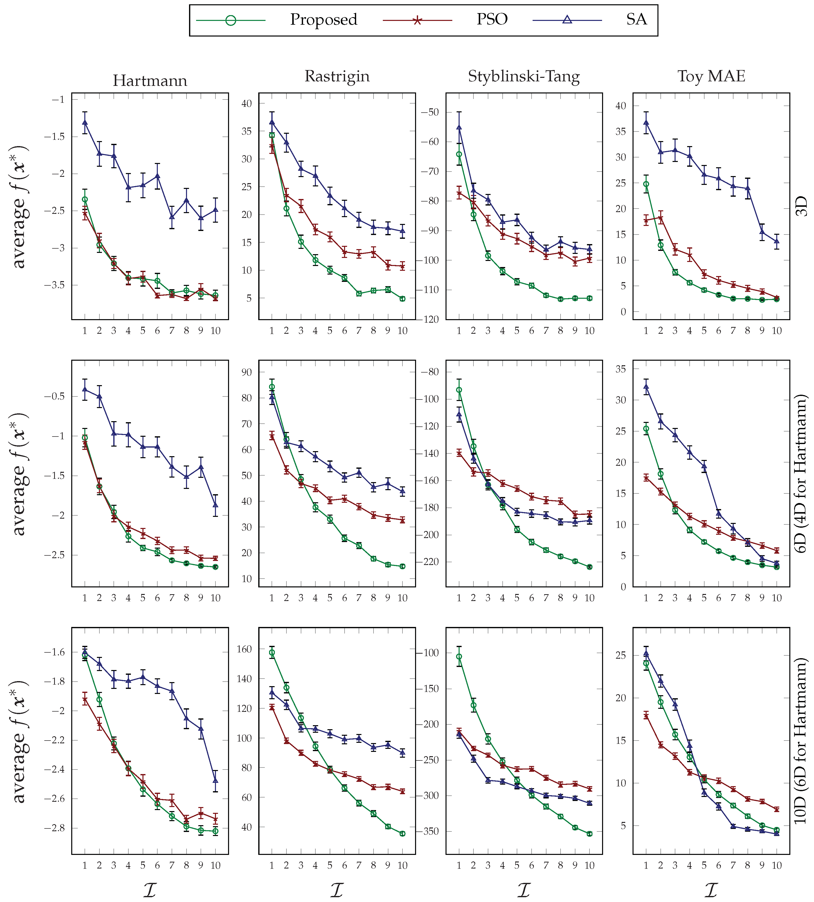
Figure 10.
Average function values of four objective functions optimized under a variable number of budget values. Each row of the figure pertains to a particular dimension size, and the error bars are calculated based on the standard error.
Figure 10.
Average function values of four objective functions optimized under a variable number of budget values. Each row of the figure pertains to a particular dimension size, and the error bars are calculated based on the standard error.
Disclaimer/Publisher’s Note: The statements, opinions and data contained in all publications are solely those of the individual author(s) and contributor(s) and not of MDPI and/or the editor(s). MDPI and/or the editor(s) disclaim responsibility for any injury to people or property resulting from any ideas, methods, instructions or products referred to in the content. |
© 2023 by the authors. Licensee MDPI, Basel, Switzerland. This article is an open access article distributed under the terms and conditions of the Creative Commons Attribution (CC BY) license (https://creativecommons.org/licenses/by/4.0/).
Share and Cite
MDPI and ACS Style
Esmaeili, A.; Ghorrati, Z.; Matson, E.T. Agent-Based Collaborative Random Search for Hyperparameter Tuning and Global Function Optimization. Systems 2023, 11, 228. https://doi.org/10.3390/systems11050228
AMA Style
Esmaeili A, Ghorrati Z, Matson ET. Agent-Based Collaborative Random Search for Hyperparameter Tuning and Global Function Optimization. Systems. 2023; 11(5):228. https://doi.org/10.3390/systems11050228
Chicago/Turabian StyleEsmaeili, Ahmad, Zahra Ghorrati, and Eric T. Matson. 2023. "Agent-Based Collaborative Random Search for Hyperparameter Tuning and Global Function Optimization" Systems 11, no. 5: 228. https://doi.org/10.3390/systems11050228
Note that from the first issue of 2016, this journal uses article numbers instead of page numbers. See further details here.