
Probabilistic Modelling of System Capabilities in Operations

Finnish Defence Research Agency, Tykkikentäntie 1, P.O. Box 10, 11311 Riihimäki, Finland
Systems 2023, 11(3), 115; https://doi.org/10.3390/systems11030115
Submission received: 23 January 2023
/
Revised: 14 February 2023
/
Accepted: 22 February 2023
/
Published: 23 February 2023
(This article belongs to the Special Issue Simplifying the Complex: Modeling and Analysis for System Design and Management)
Abstract
:We present a probabilistic method for simplifying the complexities in evaluating high-level capabilities. The method is demonstrated by using questionnaire data from a technology forecasting project. Our model defines capability as the probability of a successful operation. The model maps the actual observable capabilities to system capabilities. These theoretical quantities are used in calculating observable capability values for system combinations that are not directly evaluated as explanatory variables in the model. From the users’ point of view, the method is easy to use because the number of evaluated parameter values is minimal compared with many other methods. The model is most suited to applications where the resilience and effectiveness of systems are central factors in design and operations. Resilience is achieved by using alternative systems that produce similar capabilities. We study the limited use of alternative systems and their capabilities. We present experiments of model variations and discuss how to perform the model’s built-in consistency checks. The proposed method can be used in various applications such as comparing military system capabilities, technological investments, medical treatments and public education. Our method can add a novel view for understanding and identifying interrelations between systems’ operations.
1. Introduction
We present a probabilistic model with the primary goal of supporting understanding, analysis, communication and decision making. We demonstrate the model in three military capability areas of protection, awareness and engagement, a subset of military capabilities [1,2,3] at the highest conceptual hierarchy level. The basic model has a simple structure of necessary and alternative systems that produce capabilities on a specified hierarchy level. In this study, capability is defined as the success probability of operation in an existing or planned scenario [4]. Despite the origin of the model [4,5,6,7,8,9,10] being in military applications, it can be used in other domains where the resilience and effectiveness of systems are central factors in design and operations.
Capability-based planning (CBP) takes place under uncertainty, the results of which are definitions of capabilities in a wide range of different requirements and environments, considering economic factors and possible alternatives [11,12,13,14,15]. One definition of capability is the ability to perform a specified set of tasks [13,15]. To achieve this, writing scenarios is an important method for describing various operations and operating environments [4]. A conceptual model for defining total capability areas is used by the defence forces in many countries. Military capability areas are defined as statistically independent sets of functionalities. These functionalities form hierarchies [14,15], with the help of which the exact capability areas are defined [2]. Modelling can be performed at different levels of hierarchy and levels of detail [16,17]. The modeller decides to which level of detail the model is designed based on the requirements of the problem [2]. Throughout this study, we use the term capability area because our numerical examples in Section 3.3, Section 3.4, Section 5.1 and Section 5.2 are built on this concept.
Our probabilistic model [5,7,8,9,10] describes the capabilities of a system of systems (SoS) [1,13,15,18,19,20,21,22]. Under the general concept of capability, we consider high-level capability areas, subcapabilities, capabilities of a system of systems and individual system capabilities [7,8]. We use two types of concepts: observable capability for an actual system of systems and system capability for a theoretical decomposition of a system of systems. This is a practical approach in a case where detailed system characteristics are not available, for example, when forecasting long-term technological progress [10,23,24]. In addition, these quantities are easier for a subject expert to evaluate than the more technical individual systems’ capabilities. In the model, numerical values of capabilities are estimated probabilities of successful operations. Therefore, capabilities depend on the scenario and operation at hand. In our numerical demonstrations, we use the capability values of high-level capability areas and subcapabilities of two systems, Unmanned Aerial Vehicles (UAVs) and satellites, from a questionnaire as input data. While we have presented the model in our earlier articles, new features of the model are discussed in the context of using subsets of available systems.
We show how the method can be applied in modelling the concurrent use of subsets of available systems. Two different ways of using the model are adding (or removing) systems from an existing configuration and deploying existing systems only for a limited set of capabilities. An example of the latter is when protection and awareness capabilities are fixed for a system, for example, UAVs can only utilise their own combined protection and awareness capabilities. On a higher level, this does not exclude the possibility of deploying UAVs and satellites for producing the same capabilities.
Several extensions of the basic model show how complex interrelations can be considered. In the military context, one important application is describing systems’ self-protection capabilities. Self-protection of an alternative system is a particular component not included in the common supporting systems or in the model’s cross-terms of alternative systems. Self-protection components of alternative systems are treated as a part of the protection capability of the systems themselves.
The research question of this study is to develop a mathematical model for simplifying the evaluation of high-level capabilities in operations. The main applications are in the military domain or other critical environments where the redundancy of systems is a central means to increase the resilience [25] of a system of systems. Our goal is to develop a method for analysing trends from questionnaire data or other uncertain information. One application is technology forecasting, where technological developments are not known accurately.
Current methods, such as the Delphi method or traditional linear regression methods, require the evaluation or fitting of many variables in the corresponding models. In our model, the number of estimated numerical values is not increasing as a function of different combinations but linearly as a function of the number of alternative systems. This is achieved by modelling individual systems as independent entities that can be used as ’building blocks’ in composing different combinations of necessary and alternative systems. The proposed method is easy to use, and it is possible to visualise modelling results in real time during the evaluation process. The model is designed for describing the high-level capabilities or subcapabilities of a limited set of system functionalities. Other system engineering techniques [1,16,26] or trade-off methods [27] may be more appropriate in modelling functional system requirements or operations given that the detailed information is available. In this respect, the proposed method has limitations but it fills a specific gap in the existing literature of system engineering methods. As the concept of military utility [28] is closely related to the concept of military capability, we also present some principles of military utility in Section 2. In the literature review, we also discuss some other general topics related to our work, such as trade-off analysis [27] and technology forecasting [7,17,29].
In this study, we demonstrate the model in the military context. It is easy to find applications in many other domains. The model can be used, for example, in comparing alternative options of training and education programs [30], public procurement [31], energy use and sources [32], means of transportation [33], medical treatments [34] and technological intensity and innovation [35].
In all applications, it is worth noticing that the use of the model is based on the probabilistic definition of capability. Typically, in each application, many alternative definitions are possible. For example, in the case of evaluating training programs’ future earnings, future lifetime, meaningful work, etc., can be considered as targets for evaluating the probability of success. Moreover, what we mean by a successful event or operation must be defined. For example, USD 100,000 or above as one year’s salary is one choice for the target level. It is possible to define a discrete or continuous variable for different earning levels. Even a combination of different performance or quality levels for each evaluation target can be studied. Even multiple targets of evaluation can be considered simultaneously with different numerical levels for each target of evaluation. If needed, more than one scenario can be used in defining the situational environment.
2. Literature Review
In the literature, few mathematical models have been proposed for describing high-level capabilities. However, there is an extensive volume of literature in related fields of system engineering [20,21,22,27] and systems of systems [18]. General methodologies such as Multiple-Criteria Decision Analysis (MCDA) [36], Structural Equation Modelling (SEM) [37] and Analytic Hierarchy Process (AHP) [38] are related to our work, but they are typically used for more detailed modelling problems. A nonparametric method called Technology Forecasting with Data Envelopment Analysis (TFDEA) [29] has been used successfully in the literature. In the TFDEA method, the system is not modelled in detail, but nevertheless, the correct selection of input data is essential to obtain correct predictions.
Different trade-off methods [14,27] are often used in the decision-making process where alternatives are examined in uncertain circumstances. These decisions can vary from choosing a management style, hiring personnel and choosing the optimal systems for operations. The processes of trade-off analysis [27] consist of the following steps: understand the problem, find and define the alternatives, define the criteria, set the weights for criteria, determine the scoring, analyse the results and make decisions. These steps should be largely carried out before the modelling work, depending on the functional and technical requirements of the research question at hand. Similar phases also exist when implementing the proposed method of this study.
The concept of military utility has been proposed for the evaluation of technological systems in military operations [28]. It considers the selection of military technologies and how those technologies are used. The concept is useful in military decision-making processes such as technology foresight, operational planning, development and use of defence systems. It affects performance on the battlefield and the ability to keep up over time. Military utility is a measure of military effectiveness, affordability and suitability in specified circumstances [28]. It is derived using concept analysis [39] and is based on similar concepts in social and system sciences. With the help of the concept of military utility, it is possible to study what military capabilities are made of, the effects of the development of technologies and their use and what the effects of different military doctrines are.
In technology forecasting [17,29], the goal is to find out changes in performance and reveal the sources that improve capabilities that arise from the introduction of new systems and improvements to existing systems. Structural system modelling and probabilistic description of capabilities can be realistic forecasting methods when compared with standard mathematical methods, such as linear regression, extrapolation, factor analysis and principal component analysis.
3. Basic Iterative Model
We construct the model for a system of systems from parallel and serial subcapabilities, modelling their respective alternative and necessary capabilities. In detailed analyses, capabilities can be modelled using nested structures of parallel and serial components. In our probabilistic model, we calculate the total effect of necessary (serial) capabilities by taking the product of capability values. However, dealing with alternative (parallel) capabilities is more involved. Particularly, if more than two alternative systems are considered, the calculation is tedious without using the iterative procedure in Section 3.2.
First, we present the basic case where all systems can be described by their corresponding system capabilities that are used in the probabilistic model for calculating the capability of a capability area. These methods can be used in cases where the modelling of subsystems is difficult or there is not enough information for more detailed modelling. A practical iterative procedure is helpful in such calculations. After that, we present methods and applications for describing more complex system interrelationships.
3.1. Preliminaries
In the following, we present an iterative method for adding (or removing) new systems to a system of systems. With the iterative procedure, calculating capabilities for individual system capabilities, or for any combinations of systems, is effortless and easy. The iterative method works in a basic case when there are no complex interrelations between systems. Another use case of the concept of system capabilities is to calculate the observable capabilities of a system of systems in different scenarios or future technological progress for lower or higher system capabilities. Using the basic model, the simplest method to estimate the effects of changing system capability values is to scale the system capability values and calculate relevant observable capability values for system configurations in the operation [10].
After presenting the mathematical method for calculating system capabilities for the basic case, we present two complex variations of the model where the mathematical formulas can be solved for two or three added systems. Numerical methods can be used to solve the polynomial formulas for more than three additional systems. The order of the polynomial increases with the number of additional systems. In practice, numerical methods for three systems may be more practical, even for three new systems. The two complex cases’ internal capabilities and external system capabilities are presented in Section 5.1 and Section 5.2, respectively.
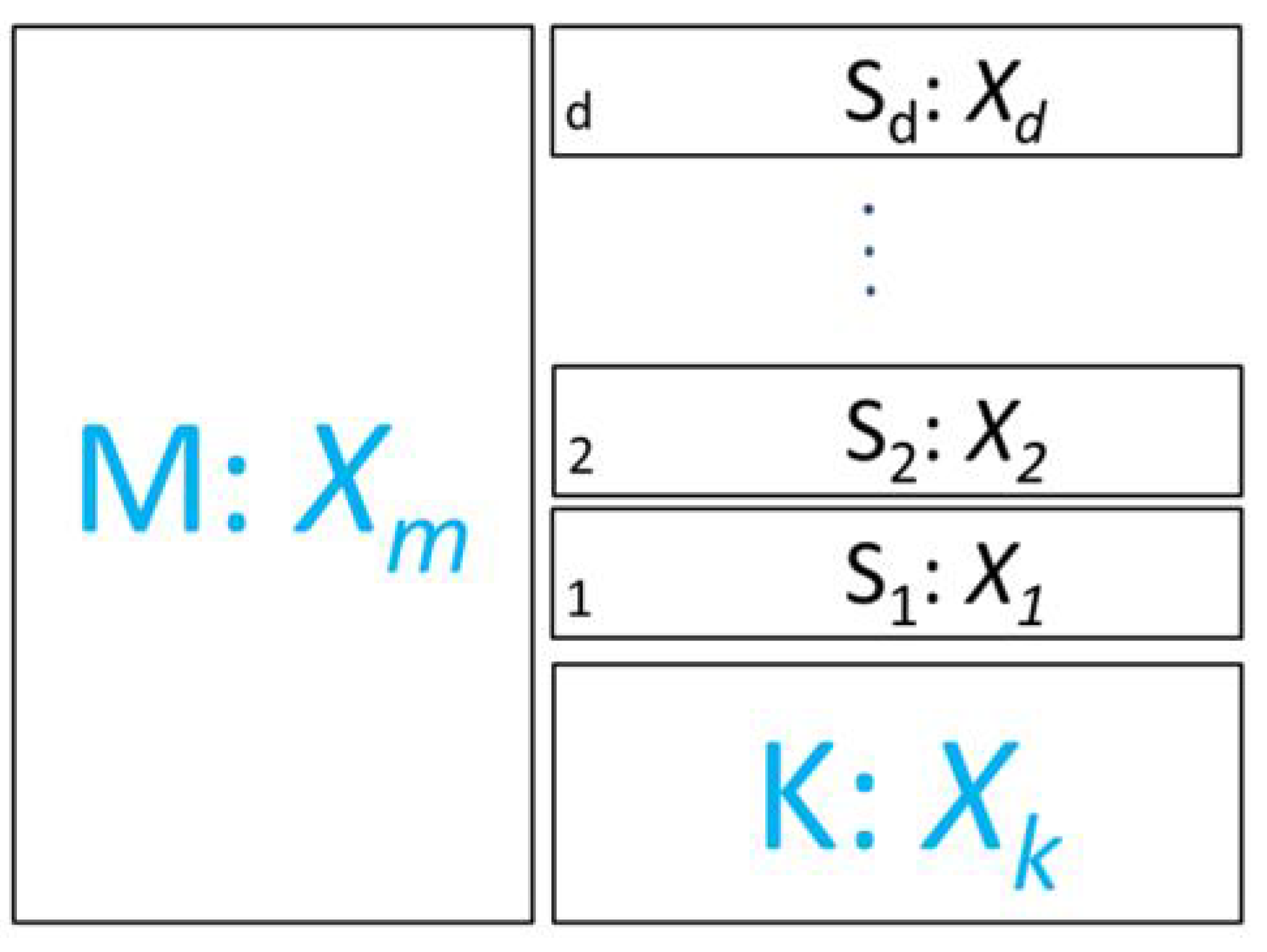
Next, we show how parallel capabilities can be computed iteratively. We denote existing capabilities by M and K, where M describes the necessary system of systems of existing capabilities and K describes the system of systems of existing alternative capabilities. This is the baseline, at time , of the analysis. New systems are introduced in addition to the existing system of systems . This configuration is shown in Figure 1. The system capabilities of systems are denoted by .
The capability value of the combined system of systems is denoted by . Because the two systems are serial, we have . The value of is approximated by a constant because new systems’ functionalities can compensate for existing capabilities. This approximation is consistent with our earlier results [6,7,9], where the quantity is a constant with an increasing value of and a decreasing value of in most cases. This is interpreted as increasing the capability of necessary system capabilities and decreasing the capability of alternative system capabilities of existing partially compensated systems. In more detailed modelling, the assumption of a constant is not made, and is replaced by , which allows changes as a function of time T.
In the context of this study, where a subset of the system of systems is in operation, the capability values of and , or the combined effect , may depend on the particular subset of deployed systems or other decisions made of the systems’ use. In these cases, corresponding effects should be evaluated and included in the model. One such example is the increased or decreased system capability of a system when deployed in different scenarios. Two methods for dealing with internal and external system capabilities are presented in Section 5.1 and Section 5.2, respectively. In the following, we assume that the value of is a constant function of time, and it is not dependent on using a subset of systems or the restrictions resulting from decision making.
3.2. The Model
We denote by the change in an observable capability value with i additional systems in a capability area. These values are obtained from questionnaire results or are evaluated through modelling or simulation methods. First, we add a new system with the capability value of in parallel with the system of systems K. According to the basic probability theory, specifically, the theorem of nonmutually exclusive events [40], the capability value of these three systems is
From Equation (1) can be solved as
In Equation (1), the left side represents the observable capability and the right side describes the system capabilities of our model. For one added system, the capability value of (or ) is required. Next, we add a second system with the capability value of . Here, we assume that is not affected when system is added. The system of systems capability value of the four systems is
where .
The value of can be solved as the value of is known:
From the above, we know that is , which is independent of the initial capability area’s capability value . This feature of the model is desirable because the initial values are the predicted values from the questionnaire. It is possible to adjust the values of without affecting the system capability values . On the other hand, the system capability values of the original defence system depend on . We presented and discussed an example of adjusting, or re-evaluating, the value of in a technological forecasting application in [6] Section 2.4. In the model, this is achieved simply by replacing by with a new parameter describing the relative change.
In general, the following iterative formula for system capabilities holds:
where
For two parallel systems, the value of can be solved with the help of the known value of :
The iterative procedure works when new parallel systems are added to the existing system of systems. The interpretation is that the capability values of an increasing set of a system of systems are known for . Alternatively, the same number of capability values of different combinations of systems are known. With the help of the model, different capability values for individual systems or combinations of systems can be calculated using the probabilistic model.
On the system level, our model makes use of the system of systems principles. In our numerical demonstrations in Section 3.3, Section 3.4, Section 5.1 and Section 5.2, two systems are assembled in parallel or series with other systems. This idea can be compared with the ideas in Martino’s more heuristic model [17]. It has some resemblance with the proposed model of this study regarding its intended use and mathematical form as a quotient. However, Martino’s model is not derived from the probability theory, and it is not specifically designed for modelling high-level capabilities or for investigating the resilience of a system of systems. The model does not involve the concept of system capability as defined in this study. As a result, all system combinations of a system of systems cannot be calculated from the same input data, as is the case in our model.
3.3. Limited Use of Systems
System capabilities may be used in a limited manner for a variety of reasons: (a) all potential capabilities are not available, (b) all potential capabilities are decided not to be used, or (c) there is not enough time or other resources to deploy all available capabilities. Respondents in the questionnaire were not informed about any restrictions on using different combinations of system capabilities. Thus, the system capability values calculated from the questionnaire data correspond to the general case where system capabilities can be used interchangeably. For example, the protection capability produced by satellites can be used to protect UAVs.
When modelling the use of subsets of potential systems, a specific question is how to take into account the reduced requirements caused by not using all of the theoretically possible systems. One important example is the absence of protection for systems not deployed in operation: If UAVs are not in operation, they do not need protection. This means that the protection capability provided to UAVs by satellites or other operative systems needs to be removed from calculations (i.e., not included).
In Figure 2, we provide an example where UAVs are not used for maintaining situational awareness, yet UAVs alone are used for engagement operations. In the example of Figure 2, systems and are used for protection, awareness and engagement, respectively. Note that the system capability values for necessary systems and alternative systems usually have different values for protection, awareness and engagement capability areas. In this particular case, the protection capability provided to UAVs’ surveillance operations by the Original Defence System (ODS) and satellites is not in effect. If this result is important, this part of the protection capability should be eliminated from the calculations. This can be carried out just by scaling the corresponding system capability value by a suitable factor or using the methods in [8,10] depending on the situation.
Removing (and adding) systems from a set of a system of systems is a built-in feature of the model—a system is removed just by setting the system capability value of the system to zero. This is straightforward when removing or adding systems and it does not change any other systems’ capability values. In many cases, this is true or, at least, a good approximation for small and moderate changes in the system composition.
In Table 1, we provide the average initial observable capability values , and for the protection, awareness and engagement capability areas, respectively. Notice, that these values are kept constant during the evaluation horizons of 1 year, 10 years and 20 years. The results of this study are conditional on this assumption. In Table 2, we provide the observable capability values from the questionnaire for the three capability areas in the three evaluation horizons for systems and , as well as the combined use of systems . Notice that, in the questionnaire, the auxiliary system of systems K is also included in the evaluations. In Table 3, system capability values , , and calculated from the model of Section 3 are provided for the three capability areas and time horizons of 1 year, 10 years and 20 years.
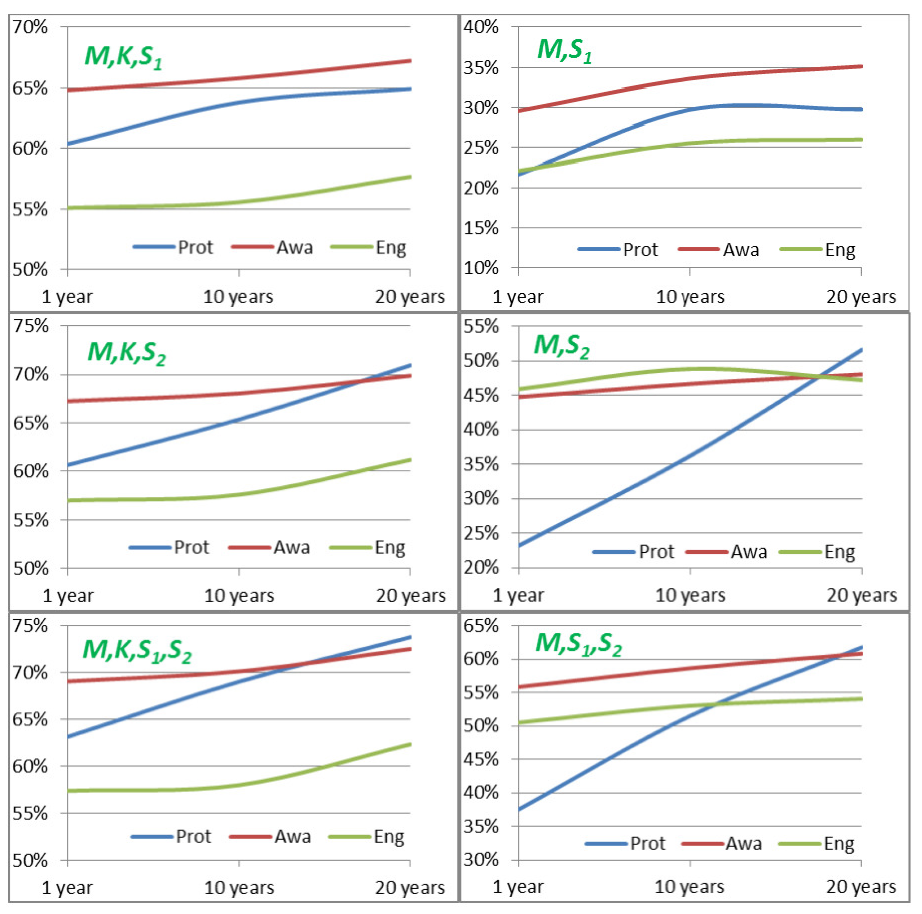
In Figure 3, the left-hand side figures show observable capability results from the questionnaire data and the right-hand side figures show observable capability results calculated from the model in Section 3. Here, we do not perform the full analysis, but some observations and conclusions can be made from the results. The calculated results (right) can reveal phenomena that are not easy to see from the original questionnaire data (left). The curves for systems highlight the important role of the system (UAVs) in producing the protection capability in the long run. In addition, system is expected to produce engagement capability both in short and long time horizons.
3.4. Limited Use of System Capabilities
Next, we assume that the use of system capabilities in an operation is not utilised with full power: We assume that a parallel system can use only its own protection and awareness capabilities in order to produce a combined capability for its two capabilities. Yet, the combined system capability, comprised of protection and awareness, can be utilised interchangeably between alternative systems. This example is particularly relevant because the protection and awareness capabilities are highly related and they support each other. Equations for the combined protection and awareness capabilities of systems and are the following:
where subscripts p and a denote protection and awareness. Note that system capability values are calculated from the basic model where restrictions were not applied. By default, the necessary system of systems M is in use, and we do not indicate that on the left-hand side of the formulas. The system capability is a multiplicative factor on the right side of the formulas. If the necessary system of systems M is not functioning, all the capability values are zero in Equation (6).
In Figure 4, the combined observable protection and awareness capability values for the limited use of systems, as defined in this section, are compared with the basic results of Section 3. The dashed lines show that the effect of limited-use systems has an effect of about five per cent for systems and about three per cent for systems , and .
4. Interrelations between Systems
In theory, different complex interrelations between systems can be modelled by modifying the system capability equations. Usually, only correcting effects can be taken into account using these approaches. In the following, three different approaches with potential applications are discussed. Another application is how to adjust a system’s capability value in different scenarios or according to future technological developments [10]. In this case, all occurrences of the system capability value are multiplied by the same adjusting factor. If changing a system capability value has no effect on other system capabilities, exact results are obtained by this method.
Modelling the higher or lower capability of the concurrent use of two systems is presented in [8]. In this study, we present two additional variants of modifying the system capability equations. They describe external and internal system capabilities. External capabilities could describe auxiliary or supporting systems that are not included in the detailed model.
It may be useful to model internal systems because, for example, self-protection can be modelled by modifying the system equations with this method. Self-protection is the protection provided by a system to itself. Improved manoeuvring or camouflage are examples of self-protection. Here, the concept of self-protecting includes only the system capability of the corresponding parallel system capability, not the multiplicative system capability :
The protection capability value of system is separated into two parts: self-protection and the remaining portion of the capability. The cross-term has only the term , describing protection without the self-protection component. In case system K also has self-protection capability, the system equation is modelled accordingly: the cross-term is multiplied by a factor .
5. Experiments with Variations of the Model
In this section, we present two different parameterisations of the model. They can approximate internal and external use capabilities as a supplementary part of modelled system capabilities. In Section 3.4, the basic model is modified by extra factors in the cross-terms of Equation (8). In Section 5.2, the basic model is modified by extra factors in the system capabilities of Equation (11).
On the grounds of these formulas, the variations can have distinguishing interpretations as real-world changes in the success probabilities of operations. Depending on the parameter value, the formulas have different relative weights for the system capability terms and the cross-terms describing the redundancy of the systems. One interpretation is to consider the two variants as internal and external capabilities that are not explicitly included in the model.
These variations of the model can also serve as a ‘What if’ analysis or as a way of testing the allowed range of parameter values in the model. We used the model’s self-consistency features to determine the parameter range in Figure 5 and Figure 6.
5.1. Internal System Capabilities
Self-protection is one of the commonly used concepts to consider protection capabilities produced by the system for its own protection. Internal capabilities can be modelled by decreasing corresponding cross-terms in the formulas. After using the relationship , we obtain from Equation (7) the following system equations for modified capability values:
Observable capability values for a capability area are , as before. Equation (8) can be expressed as a second-order equation
where the coefficients and are
Now, we can use the textbook formula of second-order polynomials for and solve the quantities and :
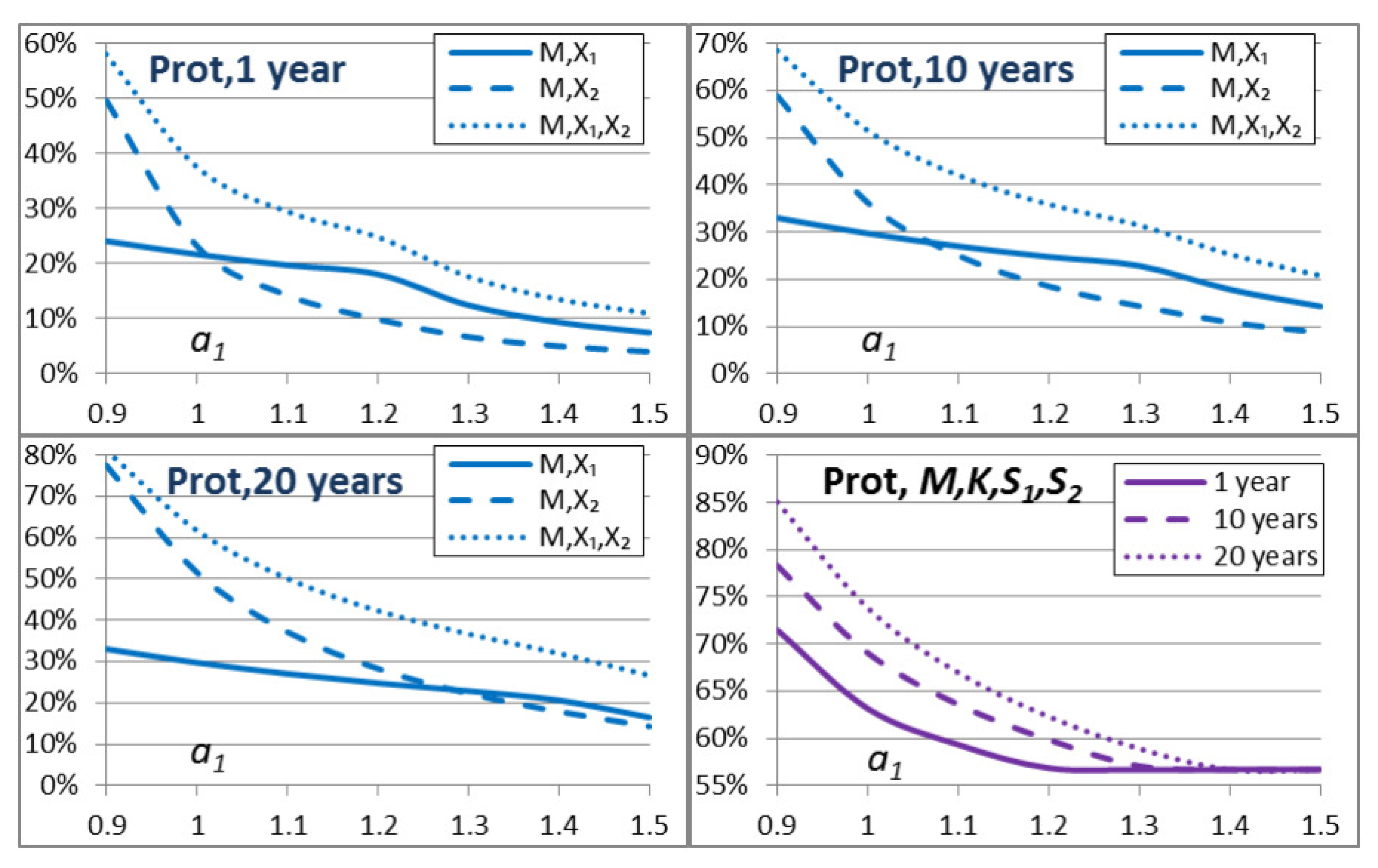
Figure 5 shows that internal capabilities have effects on observable capabilities for different time horizons. We assume that the initial capability remains constant. The observable capability values of systems , and are decreasing, but the observable capability value of is increasing as a function of the parameter value . This indicates the increasing role of the existing alternative system of systems K as a function of . The parameter value corresponds to the basic case of Section 3 and Figure 3.
5.2. External System Capabilities
Complex interrelations with external systems can be modelled by adjusting corresponding terms in the equations. External systems should be modelled in detail, but approximate methods may be sufficient for describing some external capability effects. The system capability equations and their solutions are provided in Equations (11) and (13). Practical applications are presented in Figure 6. For systems , and , the capabilities are
where and describe the changed capabilities of systems and K due to their effects via external capabilities. Notice that the consistency of the model allows also a slight decrease caused by the external system capabilities (see Section 7.2). The equation for the initial capability is replaced by . From Equation (11), the four equations and the unknown variables and , as well as , can be solved. The following quadratic equation follows for , which usual textbook methods can solve
The system capability value for system has the symmetric formulation where and are exchanged with and . On the other hand, after is known, and can be solved as
Figure 6 shows that external capabilities have an effect of decreasing observable capability values as a function of the parameter value . The observable capability values of systems , , and are all decreasing as a function of . The parameter value corresponds to the basic case of Section 3 and Figure 3.
6. Results
In this study, we presented a method for modelling system capabilities in operations. The method is based on describing the success probability of operations with different systems in use. Necessary and alternative systems are modelled with the basic probability theory. In our demonstrations, we used questionnaire data from two systems, satellites and UAVs, together with auxiliary necessary and alternative systems. General formulas for more than two alternative systems can be expressed as an iterative procedure, as explained in Section 3.2.
We use the concept of system capability for the derived quantities of the model , where the number of alternative systems is denoted by d. These quantities can be regarded approximately as independent of other systems in the scenario, that is is statistically independent of quantities . This assumption enables us to calculate all combinations of system capabilities, in addition to the ones that are direct consequences of the model input data, which in our example are the questionnaire data. It is noteworthy that we need not evaluate (or estimate) all different system combinations: it is sufficient to evaluate only values. For example, if there are two alternative systems, evaluating the four capability values is sufficient. In Section 4, we showed how to calculate the capabilities of three additional system combinations (right in Figure 3). In case there are more systems, this property of the model is even more important. A side effect is that we could have evaluated any four of the eight possible combinations of the capability (see Figure 2, where each capability area has eight combinations, including ). Certainly, one should choose the systems which can be evaluated the most easily and reliably.
Moreover, we can analyse the limited use of alternative systems such that only independent use of a system or system combination is feasible. This kind of situation can arise as a result of technical failures or operational restrictions. In Section 3.3, we demonstrated the limited use of alternative systems based on the same questionnaire data as in Section 3. This analysis also provides a lower bound for the system and observable capabilities (see the dashed lines in Figure 4).
7. Discussion
In this section, we discuss the role of observable and system capabilities. Then, we introduce the model’s unique characteristics that can be used for checking the consistency and validation of the model’s results.
7.1. Observable Capabilities and System Capabilities
In this study, we demonstrated our probabilistic modelling method by analysing an empirical questionnaire data set. The main idea of the method is to map the operation-level success probability evaluations to system-level capability values. All quantities of the model are expressed as probabilities that constitute a basis for consistency checks for the answers provided by the respondents and also for the model’s derived results. If the model yields inconsistent results, or probability values outside the range , the model does not apply, the model structure is not detailed enough, or the model parameter values are incorrect. This kind of validation test is not a common property of all system engineering models [26,27], not to mention any other models.
Formulas for more than two necessary systems are expressed as multiplicative factors for each system or a set of systems. In theory, an arbitrary configuration of a system composed of several (sub)systems can be modelled with our method. However, in practice, it may be difficult to differentiate and define all necessary and alternative functions of the analysed systems and to represent the relations of the systems as a diagram to help write the equations.
In Figure 3, Figure 4, Figure 5 and Figure 6, we chose to present the observable capability values and not the theoretical system capability values, because the former are more relevant in practice as actual quantities. System capability results can be found in our earlier studies [5,6,7,8], or they can be calculated from the formulas of these studies.
Mathematically, it is possible to evaluate the system capability values instead of the initial capability value and observable capability increment values (in our example, and ). In any case, the observable capability values expressed as success probabilities should be shown in real time to the participants of a questionnaire. Vice versa, it would also be helpful to show the calculated system capability values to the participants when the actual capability values are evaluated. This would be another consistency check because the system capability values are comparable with each other, while the evaluated capability values of different or aggregated system combinations may not be so informative.
In the proposed model, our definition of system capabilities enables calculating the observable capabilities in different combinations by using the probabilistic formulas in Section 3. This procedure is novel and original when compared with other models in the literature. For example, the heuristic model proposed by Martino [17] or any other general methods reviewed in Section 2 require the evaluation of more numerical values of model variables, typically for each combination of systems. We discussed other related literature at the end of Section 1.
On the other hand, if the combined use of systems is complicated, that is, it does not obey the rule of nonmutually exclusive events of the probability theory [40], systems should be modelled in a lower level of subsystems. This may not be possible in all cases, and then other methods are more suitable, for example, the system engineering methods mentioned in Section 2. Even though, in theory, it is possible to model a system on a detailed level, it may be difficult to conceptually define the success probabilities in the model or to describe the interrelations between systems with basic probabilistic formulas. This can be a limitation of the proposed model. In this study, we also discussed how these kinds of complexities could be modelled approximately in some cases by introducing additional phenomenological parameters in the model.
7.2. Consistency and Validation of the Results
Because the concept of capability is defined as a probability, the model has a built-in consistency check for the modelling results. Formulas that map the observable capability values to the theoretical system capabilities can produce system capability values that are negative or higher than 1. If we hold on to the probability interpretation, output variables must be in the range .
In our original questionnaire, for example, the value for the protection capability for a 10 year forecasting period in Scenario 1 had the value . We have discussed possible causes for this nonphysical result in [5] and in Section 2.4 in [6]. Note that the overflow does not come up in this work, as we analyse average results over the three scenarios of the original questionnaire compensating for individual outliers in the calculations. Outliers are possible because there were only 10 respondents in the questionnaire, which is a low number with which to obtain statistically accurate results. In summary, there are several possible explanations for the discrepancy: (a) too low a number of participants in the questionnaire, (b) a bias in a significant portion of input data [10], (c) protection capability as a multifaceted concept that is difficult to figure out and evaluate [5], (d) the model is too simple to describe the protection capability, etc.
The model for a system of systems consisting of d parallel systems in addition to the auxiliary parallel system of systems K needs explanatory variables for auxiliary necessary systems, auxiliary alternative systems and d alternative systems. The model has degrees of freedom in how to choose the evaluated explanatory variables. For example, in the case of two alternative systems, we have eight possible variables. We can use the four leftover combinations of systems for checking purposes, or we can evaluate more than the required number of observable capability values. It would be informative to visualise all response variables of the model, both observable capabilities and theoretical system capabilities.
Moreover, the system capability values can be used for consistency checks because they are expressed as separate quantities which can be compared with each other, unlike the cumulative capability values in the iterative process explained in Section 3. The iterative algorithm is based on adding new systems into the system of systems one by one. As we have defined capability as the probability of a successful operation, added alternative systems produce less additional observable capability because redundancy is increasing. This emphasises the importance of monitoring the system capability values during the evaluation process and tuning evaluated values when needed. Notice that the formulas in Section 3 apply only to the cumulative method of iteratively adding a system to an existing set of systems. If the observable capabilities are handled in some other order, the formulas must be derived for that case.
8. Conclusions
Our proposed probabilistic models can assist in simplifying subjective complexities and providing descriptions that can be used as heuristics to understand and manage systems and their capabilities. Although the approach has some limitations in describing detailed complicated structures of systems, it can be useful in many applications, for example, in forecasting long-term technological progress, where detailed information about systems’ characteristics and performance is not available. On the other hand, the method can be used as a tool to analyse questionnaire results where the opinions or subjective views of the participants are surveyed.
The novelty of our work is in presenting a probabilistic method for simplifying the complexities in evaluating the high-level capabilities defined as success probabilities in operations. This is accomplished by using the basic probability theory and introducing the concept of system capability. In the model, the system capabilities are approximately independent of other system capabilities in the scenario. In other words, the model maps the actual observable capabilities to independent system capabilities that can be used in calculating capability values for new system combinations that have not been evaluated in the original questionnaire or estimated in a submodel. The new system combinations can be either a combination of several theoretical system capabilities or an observable system of systems capabilities. This enables calculating capabilities of different system combinations from the same input data without evaluating all different combinations, for example, contrary to the Delphi method [24].
The method is easy to use from the user’s point of view. The number of different numerical values to be evaluated is small compared with many other models in the literature. Yet, the model provides capability values for system configurations that have not been directly included in the evaluation process. The model can be used to present these modelling results and visualisations simultaneously with the evaluation work. These features of the model help to check and validate the evaluations.
We demonstrated the use of system capabilities in three different ways. We calculated the capability values of system combinations that were not directly considered in the questionnaire, and we calculated the effects of the limited use of systems as alternatives in producing capabilities in operations. Thirdly, we experimented with variants of the model by using the same questionnaire data as input. These calculations can be used to test the boundaries of the model’s parameter range and to examine how sensitive the model results are to variations of the model.
We discussed how the consistency of the results can be checked and how the modelling results can be validated by monitoring the calculated system capabilities of individual systems and combinations of systems. We used consistency tests in selecting the viable parameter ranges of our model variants of internal and external capabilities.
There are many practical applications where our method can be used in modelling the success probabilities of operations or as a complementary instrument to other system engineering methods. The method can be used in almost all branches of activities from technological investments to medical treatments and public education. Our method can add a novel view for understanding and identifying interrelations between systems’ operations that can be useful in validating other models being used and their parameter values.
Funding
This research received no external funding.
Data Availability Statement
Capability changes from the questionnaire data: Table 3 in https://doi.org/10.1109/PICMET.2015.7273141.
Acknowledgments
We acknowledge useful discussions with Marko Suojanen.
Conflicts of Interest
The authors declare no conflict of interest.
Abbreviations
| AHP | Analytic Hierarchy Process |
| MCDA | Multiple-Criteria Decision Analysis |
| SEM | Structural Equation Modelling |
| TFDEA | Technology Forecasting with Data Envelopment Analysis |
| CBP | Capabilities-Based Planning |
| SoS | System of Systems |
| UAV | Unmanned Aerial Vehicle |
| Prot | Protection Capability Area |
| Awa | Awareness Capability Area |
| Eng | Engagement Capability Area |
| ODS | Original Defence System |
| Symbols | |
| Initial capability of a capability area | |
| Increment of the capability when System 1 is added | |
| to the system of systems | |
| Increment of the capability when System 2 is added | |
| to the system of systems | |
| Increment of the capability with Systems 1 and 2 added | |
| to the system of systems | |
| System 1 | |
| System 2 | |
| M | Necessary System M |
| K | Alternative System K |
| Capability of System 1 | |
| Capability of System 2 | |
| Capability of concurrent use of Systems 1 and 2 | |
| Capability of System M | |
| Capability of System K | |
| System Capability of concurrent use of systems | |
| Increment of the capability when Systems are added to | |
| the system of systems | |
| Coefficients used in the extensions of the model in Section 5 |
References
- Koivisto, J.; Ritala, R.; Vilkko, M. Conceptual model for capability planning in a military context—A systems thinking approach. Syst. Eng. 2022, 25, 457–474. [Google Scholar] [CrossRef]
- Smith, C.; Oosthuizen, R. Applying systems engineering principles towards developing defence capabilities. Incose Int. Symp. 2012, 22, 972–986. [Google Scholar] [CrossRef]
- Ding, J.; Si, G.; Ma, J.; Wang, Y.; Wang, Z. Mission evaluation: Expert evaluation system for large-scale combat tasks of the weapon system of systems. Sci. China Inf. Sci. 2018, 61, 1–19. [Google Scholar] [CrossRef]
- Suojanen, M.; Kuikka, V.; Nikkarila, J.P.; Nurmi, J. An example of scenario-based evaluation of military capability areas An impact assessment of alternative systems on operations. In Proceedings of the 2015 Annual IEEE Systems Conference (SysCon) Proceedings, Vancouver, BC, Canada, 13–16 April 2015; pp. 601–607. [Google Scholar] [CrossRef]
- Kuikka, V. Methods for Modeling Military Capabilities. In Proceedings of the 2019 IEEE International Systems Conference (SysCon), Orlando, FL, USA, 8–11 April 2019; pp. 1–6. [Google Scholar] [CrossRef]
- Kuikka, V. Modeling of Military Capabilities, Combat Outcomes and Networked Systems with Probabilistic Methods, Number 44 in National Defence University, Series 1. Research Publications. Ph.D. Thesis, National Defence University, Helsinki, Finland, 2021. [Google Scholar]
- Kuikka, V.; Nikkarila, J.P.; Suojanen, M. A technology forecasting method for capabilities of a system of systems. In Proceedings of the 2015 Portland International Conference on Management of Engineering and Technology (PICMET), Portland, OR, USA, 2–6 August 2015; pp. 2139–2150. [Google Scholar] [CrossRef]
- Kuikka, V. Number of System Units Optimizing the Capability Requirements through Multiple System Capabilities. J. Appl. Oper. Res. 2016, 8, 26–41. [Google Scholar]
- Kuikka, V.; Suojanen, M. Modelling the impact of technologies and systems on military capabilities. J. Battlef. Technol. 2014, 17, 9–16. [Google Scholar]
- Kuikka, V.; Nikkarila, J.P.; Suojanen, M. Dependency of Military Capabilities on Technological Development. J. Mil. Stud. 2015, 6, 29–58. [Google Scholar] [CrossRef]
- Davis, P.K. Analytic Architecture for Capabilities-Based Planning, Mission-System Analysis, and Transformation; RAND National Defense Research Inst.: Santa Monica, CA, USA, 2002. [Google Scholar]
- Lam, S.; Pagotto, J.; Pogue, C.; Hales, D. A Metric Framework for Capability Definition, Engineering and Management: Seventeenth Annual International Symposium of the International Council On Systems Engineering (INCOSE) 24–28 July 2007. In Proceedings of the INCOSE International Symposium; Wiley Online Library: Hoboken, NJ, USA, 2007; Volume 17, pp. 969–980. [Google Scholar]
- Biltgen, P.T. A Methodology for Capability-Based Technology Evaluation for Systems-of-Systems. Ph.D. Thesis, Aerospace Engineering, Tulsa, OK, USA, 2007. [Google Scholar]
- Biltgen, P.; Ender, T.; Mavris, D. Development of a Collaborative Capability-Based Tradeoff Environment for Complex System Architectures. In Proceedings of the 44th AIAA Aerospace Sciences Meeting and Exhibit, Reno, Nevada, 9–12 January 2006; p. 728. [Google Scholar]
- Biltgen, P.T. Uncertainty quantification for capability-based systems-of-systems design. In Proceedings of the 26th International Congress of the Aeronautical Sciences, Anchorage, AK, USA, 14–19 September 2008; ICAS2008-1.3. Volume 3. [Google Scholar]
- Sage, A.P.; Cuppan, C.D. On the systems engineering and management of systems of systems and federations of systems. Inf. Knowl. Syst. Manag. 2001, 2, 325–345. [Google Scholar]
- Martino, J.P. An Introduction to Technological Forecasting; Gordon and Breach: London, UK, 1972. [Google Scholar]
- Martin, J.; Axelsson, J.; Carlson, J.; Suryavedara, J. The Capability Concept in the Context of Systems of Systems: A Systematic Literature Review. In Proceedings of the 2022 IEEE International Symposium on Systems Engineering (ISSE), Vienna, Austria, 24–26 October 2022; pp. 1–18. [Google Scholar] [CrossRef]
- Carr, R.; Eyre, R. Maximising coherence in the integration of systems-of-systems. In Proceedings of the IET Forum on Capability Engineering-At Home and Abroad, London, UK, 7 November 2006. [Google Scholar]
- Lane, J.A. System of systems capability to requirements engineering. In Proceedings of the 2014 9th International Conference on System of Systems Engineering (SOSE), Glenelg, SA, Australia, 9–13 June 2014; pp. 91–96. [Google Scholar] [CrossRef]
- Petnga, L.; Gasque, T. Capability-driven Formulation of System of Systems Core Competencies. In Proceedings of the 2019 14th Annual Conference System of Systems Engineering (SoSE), Anchorage, AK, USA, 19–22 May 2019; pp. 119–124. [Google Scholar] [CrossRef]
- Bin, Z.; Ruijun, L.; Jing, Z.; Wei, Z.; Lijian, T. Fundamental measures of the complex SoS capability oriented to the planning and decision-making of engineering construction. In Proceedings of the 2014 9th International Conference on System of Systems Engineering (SOSE), Glenelg, SA, Australia, 9–13 June 2014; pp. 19–24. [Google Scholar] [CrossRef]
- Kim, B.S. Measuring Technological Change–Concept, Methods, and Implications. Technol. Chang. 2012, 10, 2015. [Google Scholar]
- Rowe, G.; Wright, G. Expert Opinions in Forecasting: The Role of the Delphi Technique. In Principles of Forecasting: A Handbook for Researchers and Practitioners; Armstrong, J.S., Ed.; Springer: Boston, MA, USA, 2001; pp. 125–144. [Google Scholar] [CrossRef]
- Wade, Z.; Goerger, S.; Parnell, G.S.; Pohl, E.; Specking, E. Incorporating resilience in an integrated analysis of alternatives. Mil. Oper. Res. 2019, 24, 5–16. [Google Scholar]
- Mobus, G.E.; Kalton, M.C. Principles of Systems Science; Understanding Complex Systems; Springer: New York, NY, USA, 2014. [Google Scholar]
- Parnell, G.S. Trade-Off Analytics: Creating and Exploring the System Tradespace; John Wiley & Sons, Inc.: Hoboken, NJ, USA, 2016. [Google Scholar]
- Andersson, K.; Bang, M.; Marcus, C.; Persson, B.; Sturesson, P.; Jensen, E.; Hult, G. Military utility: A proposed concept to support decision-making. Technol. Soc. 2015, 43, 23–32. [Google Scholar] [CrossRef]
- Inman, O.L.; Anderson, T.R.; Harmon, R.R. Predicting US jet fighter aircraft introductions from 1944 to 1982: A dogfight between regression and TFDEA. Technol. Forecast. Soc. Chang. 2006, 73, 1178–1187. [Google Scholar] [CrossRef]
- Walker, M.; Unterhalter, E. The capability approach: Its potential for work in education. Amartya Sen’S Capab. Approach Soc. Justice Educ. 2007, 1–17. [Google Scholar]
- Flynn, A.; Davis, P. Explaining SME participation and success in public procurement using a capability-based model of tendering. J. Public Procure. 2017. [Google Scholar] [CrossRef]
- Day, R.; Walker, G.; Simcock, N. Conceptualising energy use and energy poverty using a capabilities framework. Energy Policy 2016, 93, 255–264. [Google Scholar] [CrossRef]
- Callefi, M.H.B.M.; Ganga, G.M.D.; Godinho Filho, M.; Queiroz, M.M.; Reis, V.; dos Reis, J.G.M. Technology-enabled capabilities in road freight transportation systems: A multi-method study. Expert Syst. Appl. 2022, 203, 117497. [Google Scholar] [CrossRef]
- Zawadzki, M.; Montibeller, G. A framework for supporting health capability-based planning: Identifying and structuring health capabilities. Risk Anal. 2022. [Google Scholar] [CrossRef] [PubMed]
- Zawislak, P.A.; Fracasso, E.M.; Tello-Gamarra, J. Technological intensity and innovation capability in industrial firms. Innov. Manag. Rev. 2018, 15, 189–207. [Google Scholar] [CrossRef]
- Tzeng, G.H.; Shen, K.Y. New Concepts and Trends of Hybrid Multiple Criteria Decision Making; CRC Press: Boca Raton, FL, USA, 2017. [Google Scholar]
- Cheung, M.W.L. Meta-Analysis: A Structural Equation Modeling Approach; John Wiley & Sons: Hoboken, NJ, USA, 2015. [Google Scholar]
- Karayalcin, I.I. The Analytic Hierarchy Process: Planning, Priority Setting, Resource Allocation; Thomas, L., Ed.; SAATY McGraw-Hill: New York, NY, USA, 1980. [Google Scholar]
- Goertz, G.; Mahoney, J. Concepts and measurement: Ontology and epistemology. Soc. Sci. Inf. 2012, 51, 205–216. [Google Scholar] [CrossRef]
- Florescu, I. Probability and Stochastic Processes; John Wiley & Sons, Inc.: Hoboken, NJ, USA, 2014. [Google Scholar]
Figure 1.
Structure of the model with necessary and alternative systems. Systems of systems are denoted by M and K and their system capabilities by and , respectively. The system capabilities of systems are denoted by .
Figure 1.
Structure of the model with necessary and alternative systems. Systems of systems are denoted by M and K and their system capabilities by and , respectively. The system capabilities of systems are denoted by .

Figure 2.
There are 343 alternative combinations of system capabilities for creating the total capability of the three example capability areas. One alternative path is indicated by the red colour as an example. Observable capabilities can be calculated by including the necessary system of systems M with the system capability for the capability areas and one of the alternative 343 paths of the graph.

Figure 3.
Observable capability results for six combinations for three capability areas. Figures on the left are direct results from the questionnaire data and figures on the right are results from the model.
Figure 3.
Observable capability results for six combinations for three capability areas. Figures on the left are direct results from the questionnaire data and figures on the right are results from the model.

Figure 4.
Limited system capability results of four combinations for protection and awareness capability areas (see Section 3.4).
Figure 4.
Limited system capability results of four combinations for protection and awareness capability areas (see Section 3.4).
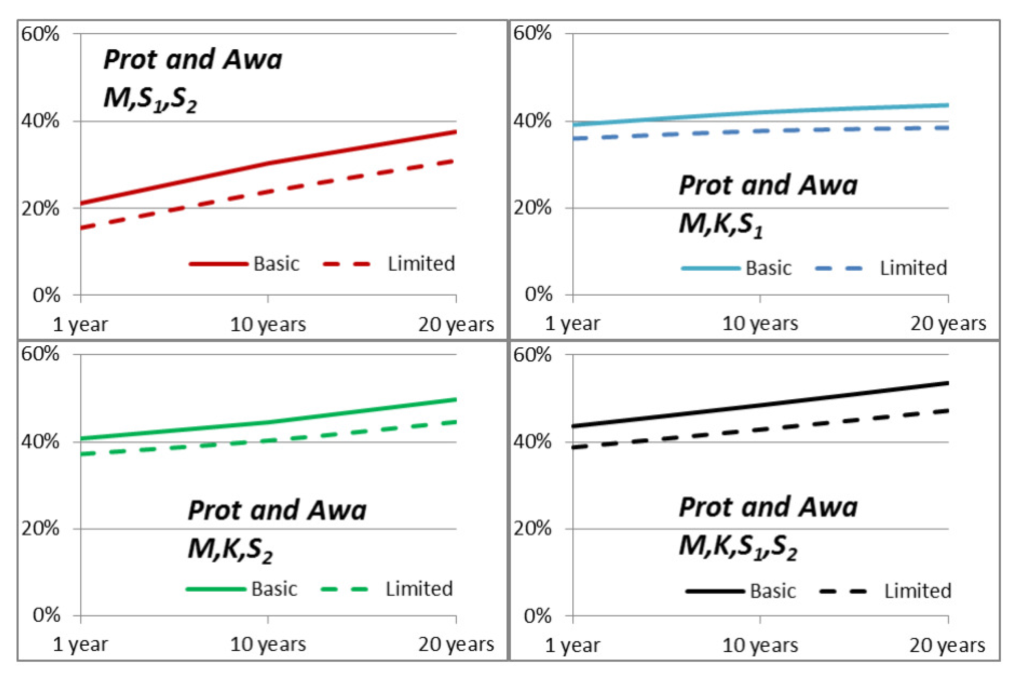
Figure 5.
Protection capability as a function of the model parameter for 1 year, 10 years and 20 years. The model in Equation (8) can be interpreted through internal capabilities of systems, for example, self-protection in Section 5.1. In these calculations, we used the parameter values and (here, we assume that both systems and have a self-protection component).
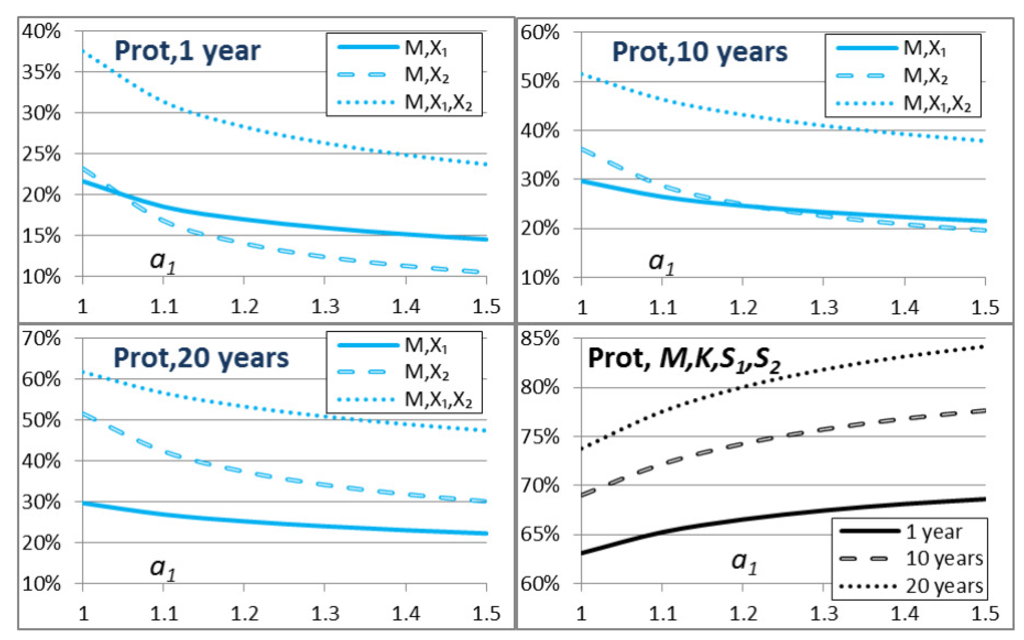
Figure 6.
Effects of external capabilities (see Section 5.2). Small humps in the figures are a result of consistency checks where we selected the + or − sign solution of the second-order polynomial of Equation (12). In these calculations, we used the parameter values of and .
Figure 6.
Effects of external capabilities (see Section 5.2). Small humps in the figures are a result of consistency checks where we selected the + or − sign solution of the second-order polynomial of Equation (12). In these calculations, we used the parameter values of and .


Table 1.
Average initial values over three scenarios for three capability areas.
| Prot | Awa | Eng |
|---|---|---|
| 0.567 | 0.600 | 0.533 |
Table 2.
Average values over three scenarios of the questionnaire results for three capability areas, two systems and three forecasting periods. In the questionnaire, the number of system units was not fixed. System of systems K is included in all of these evaluations.
Table 2.
Average values over three scenarios of the questionnaire results for three capability areas, two systems and three forecasting periods. In the questionnaire, the number of system units was not fixed. System of systems K is included in all of these evaluations.
| Capability Area | Systems | 1 Year | 10 Years | 20 Years |
|---|---|---|---|---|
| Prot | Sat | 0.037 | 0.071 | 0.082 |
| UAV | 0.040 | 0.087 | 0.143 | |
| Sat and UAV | 0.065 | 0.124 | 0.171 | |
| Awa | Sat | 0.048 | 0.058 | 0.072 |
| Uav | 0.073 | 0.081 | 0.099 | |
| Sat and UAV | 0.091 | 0.101 | 0.125 | |
| Eng | Sat | 0.018 | 0.022 | 0.043 |
| Uav | 0.037 | 0.043 | 0.079 | |
| Sat and UAV | 0.040 | 0.046 | 0.090 |
Table 3.
System capability values calculated from the model. The three rows in the table correspond to the three time horizons of the valuations 1 year, 10 years and 20 years.
Table 3.
System capability values calculated from the model. The three rows in the table correspond to the three time horizons of the valuations 1 year, 10 years and 20 years.
| Prot | Awa | Eng | |||||||||
|---|---|---|---|---|---|---|---|---|---|---|---|
| 0.317 | 0.339 | 0.685 | 0.828 | 0.413 | 0.625 | 0.716 | 0.838 | 0.382 | 0.792 | 0.580 | 0.920 |
| 0.398 | 0.486 | 0.746 | 0.760 | 0.463 | 0.644 | 0.725 | 0.827 | 0.438 | 0.836 | 0.584 | 0.913 |
| 0.380 | 0.659 | 0.784 | 0.723 | 0.465 | 0.636 | 0.756 | 0.794 | 0.407 | 0.738 | 0.640 | 0.834 |
Disclaimer/Publisher’s Note: The statements, opinions and data contained in all publications are solely those of the individual author(s) and contributor(s) and not of MDPI and/or the editor(s). MDPI and/or the editor(s) disclaim responsibility for any injury to people or property resulting from any ideas, methods, instructions or products referred to in the content. |
© 2023 by the author. Licensee MDPI, Basel, Switzerland. This article is an open access article distributed under the terms and conditions of the Creative Commons Attribution (CC BY) license (https://creativecommons.org/licenses/by/4.0/).
Share and Cite
MDPI and ACS Style
Kuikka, V. Probabilistic Modelling of System Capabilities in Operations. Systems 2023, 11, 115. https://doi.org/10.3390/systems11030115
AMA Style
Kuikka V. Probabilistic Modelling of System Capabilities in Operations. Systems. 2023; 11(3):115. https://doi.org/10.3390/systems11030115
Chicago/Turabian StyleKuikka, Vesa. 2023. "Probabilistic Modelling of System Capabilities in Operations" Systems 11, no. 3: 115. https://doi.org/10.3390/systems11030115
Note that from the first issue of 2016, this journal uses article numbers instead of page numbers. See further details here.