


An Artificial Neural Network Model for Project Effort Estimation

Abstract
1. Introduction
2. Literature Review
2.1. Project Effort Drivers
2.2. Prediction Techniques in Project Effort Estimation
2.3. Optimization of ANN Architecture
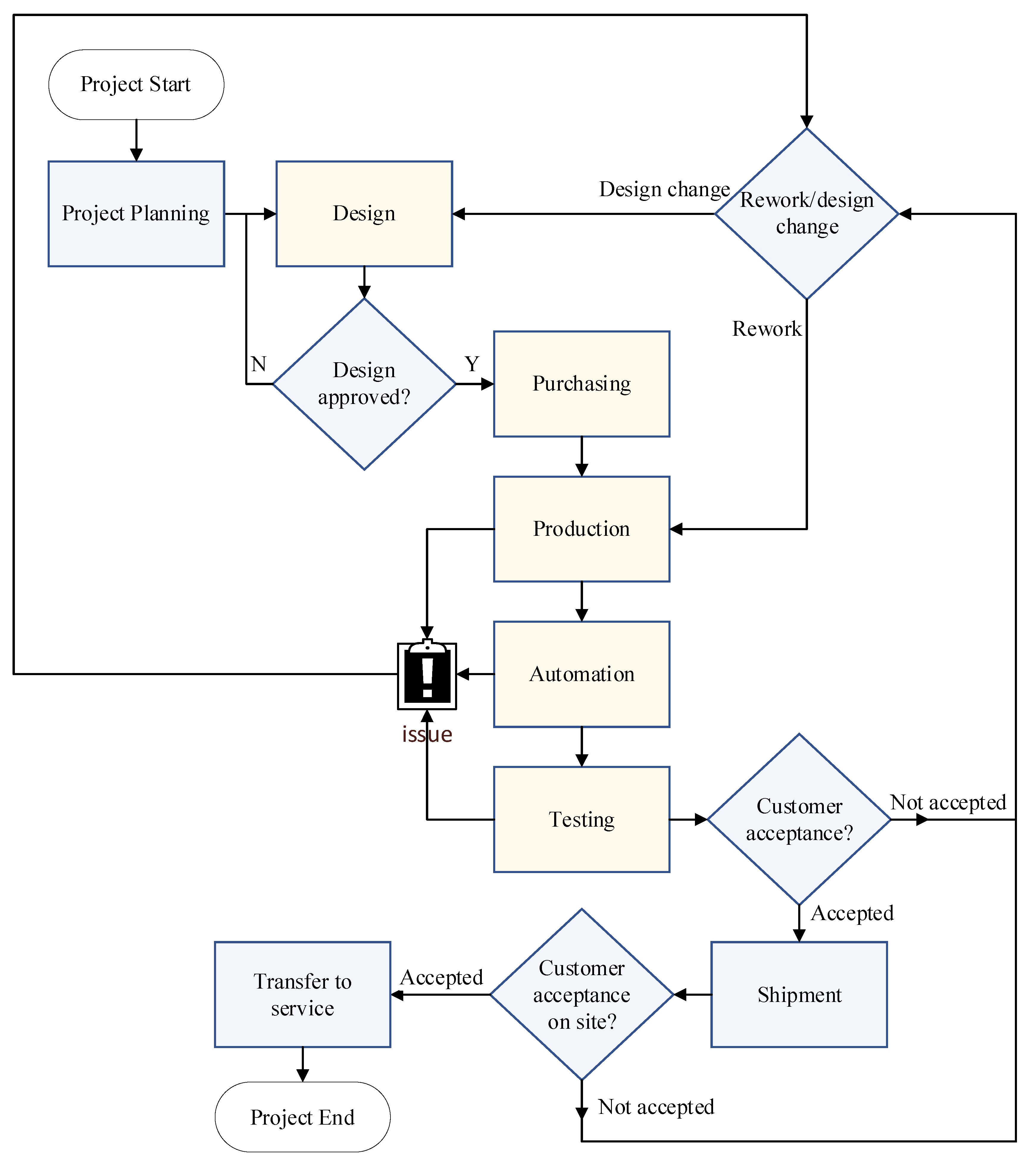
3. Methodology
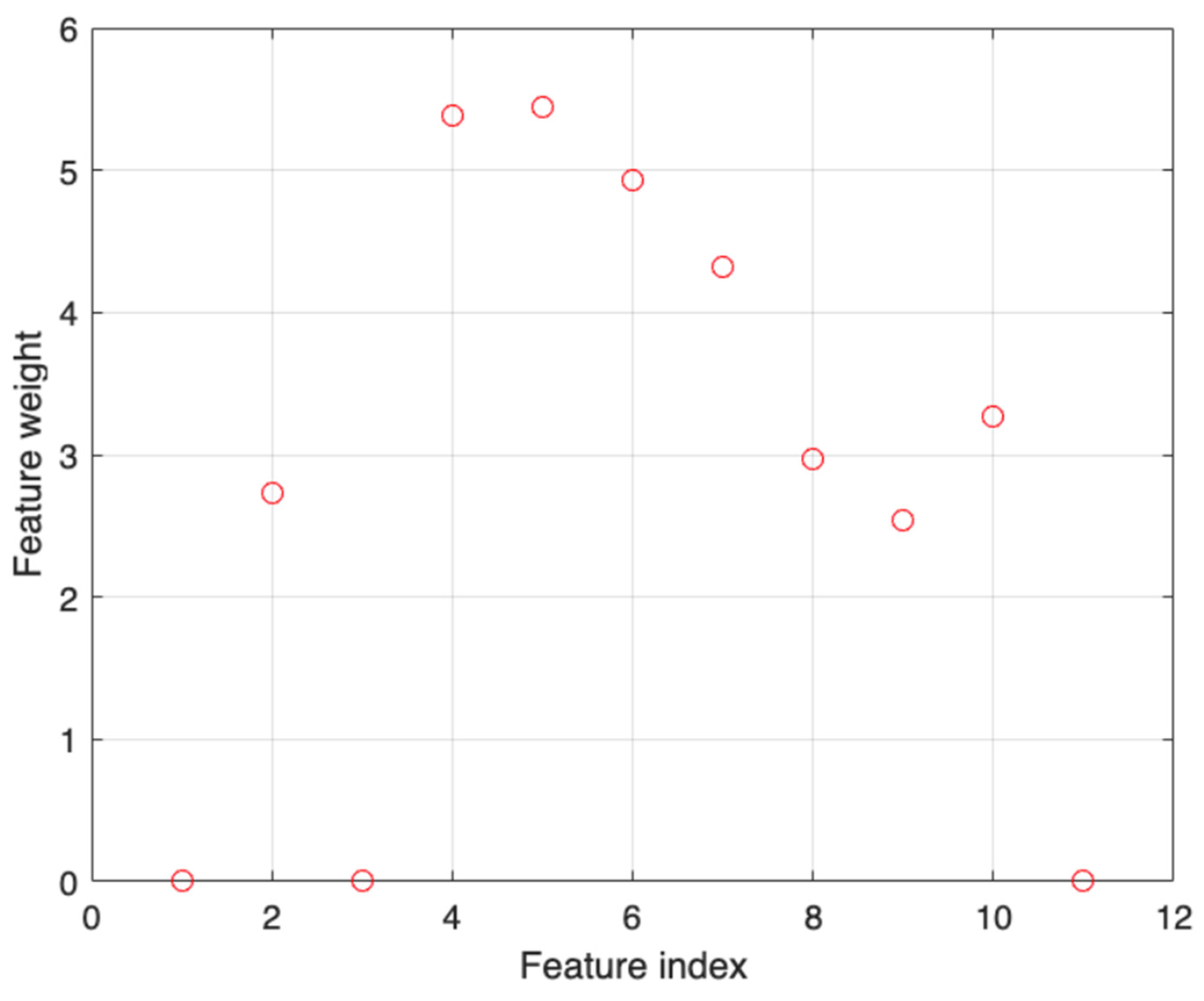
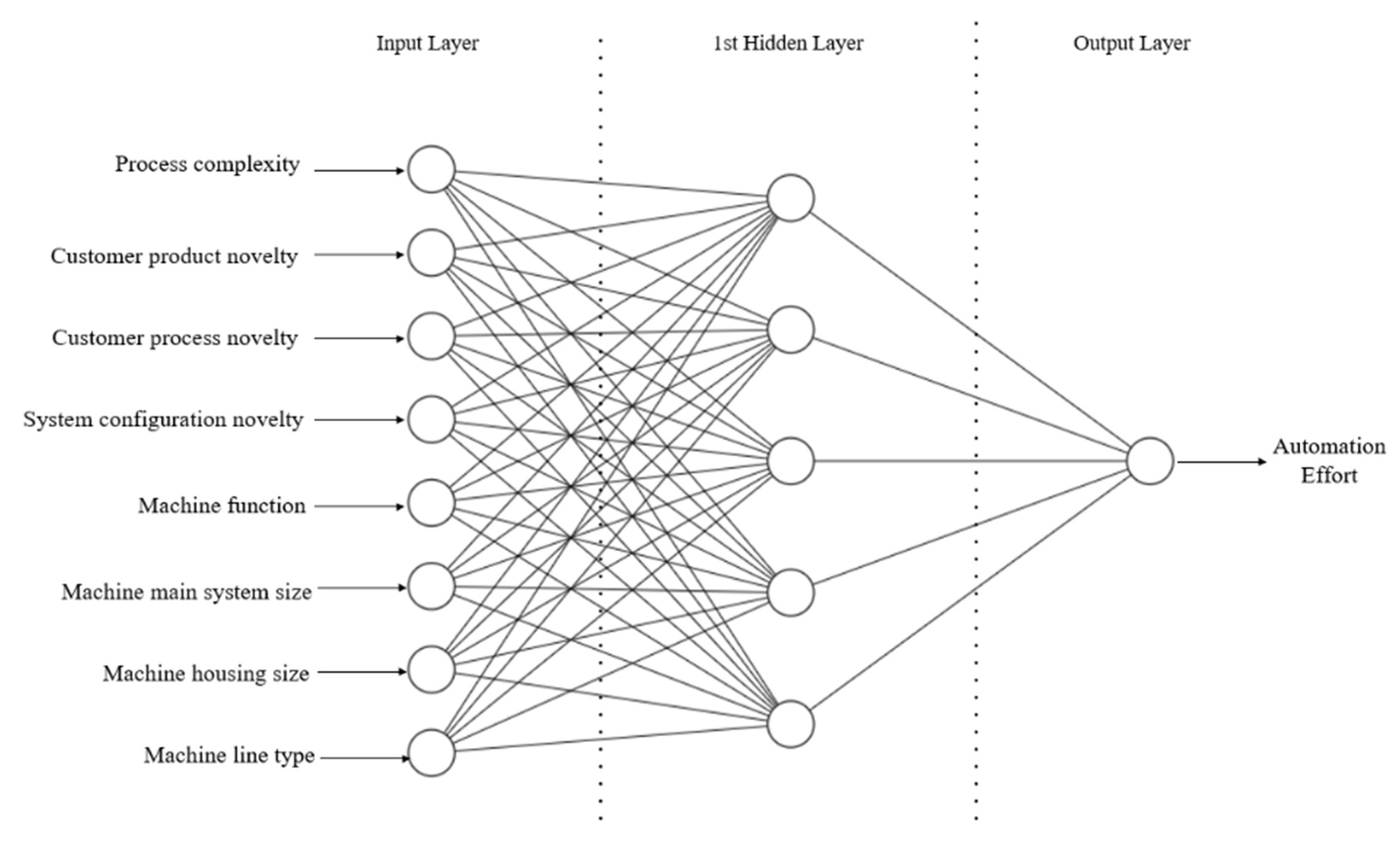
3.1. Input Selection for the Proposed ANN Model
- Hardware complexity;
- Process complexity;
- Customer type;
- Customer product novelty;
- Customer process novelty;
- System configuration novelty;
- Machine function;
- Machine main system size;
- Machine housing size;
- Machine line type;
- Outsource usage for production.
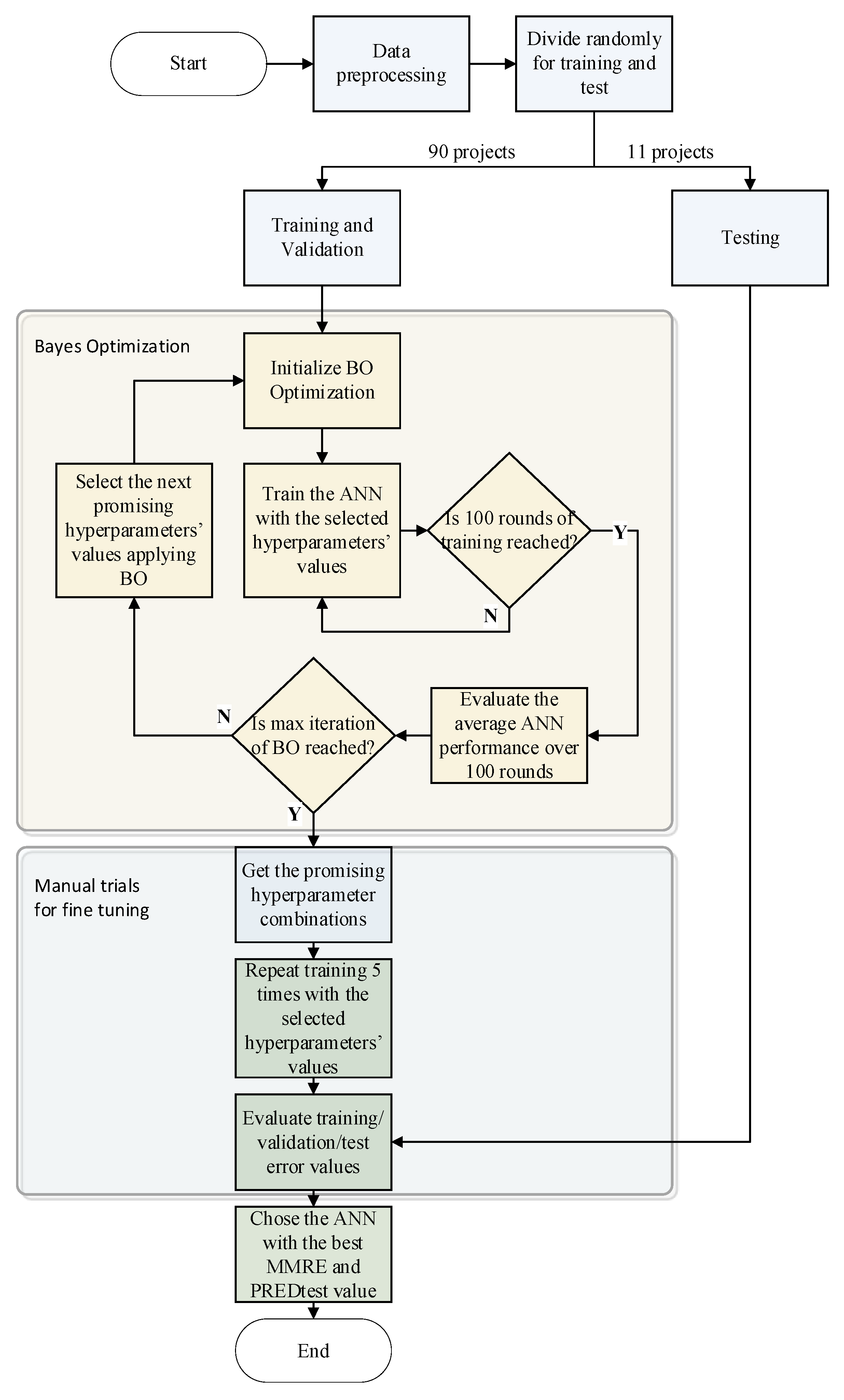
3.2. Hyperparameter Optimization of the Proposed ANN
4. Results and Discussion
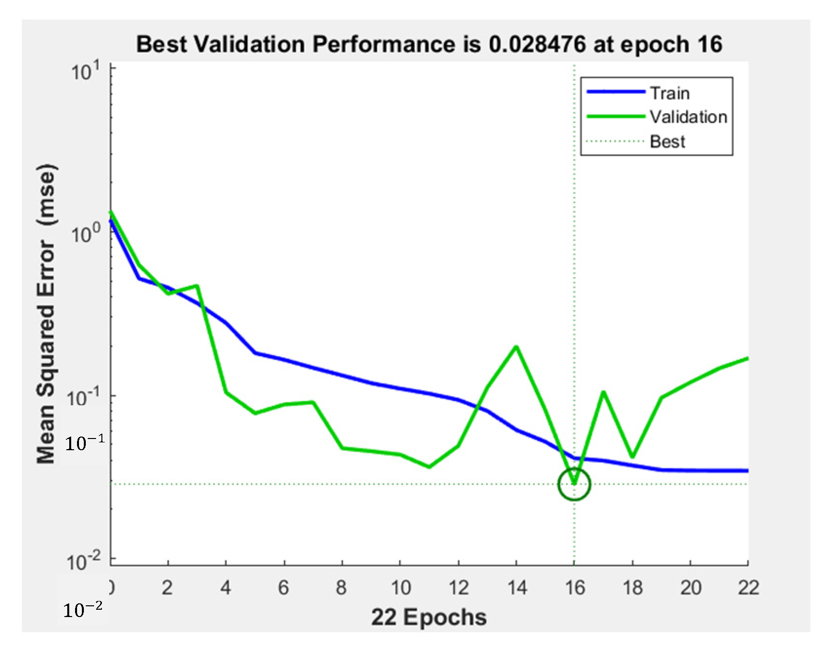
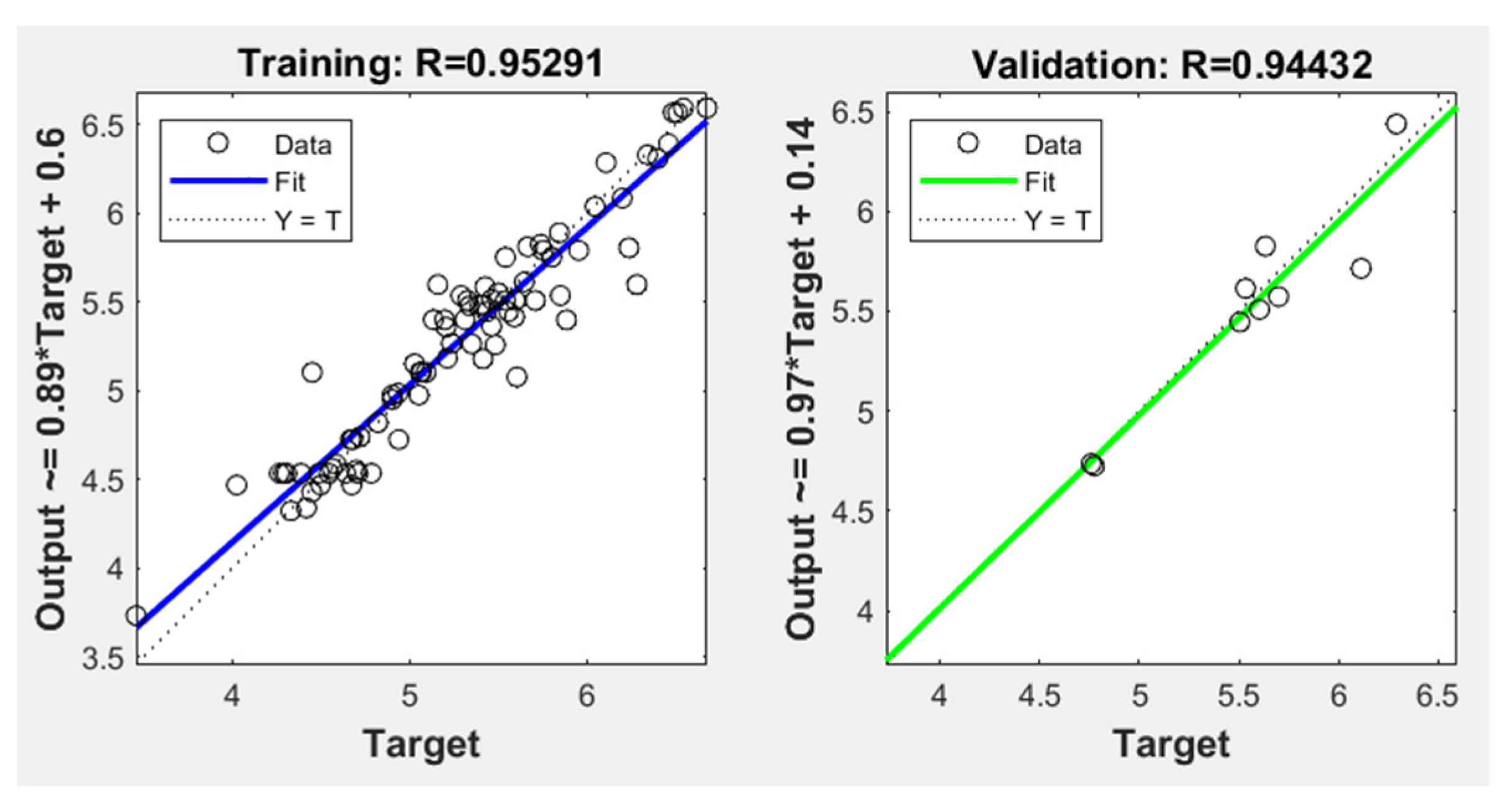
4.1. The Architecture and Performance of the Proposed ANN
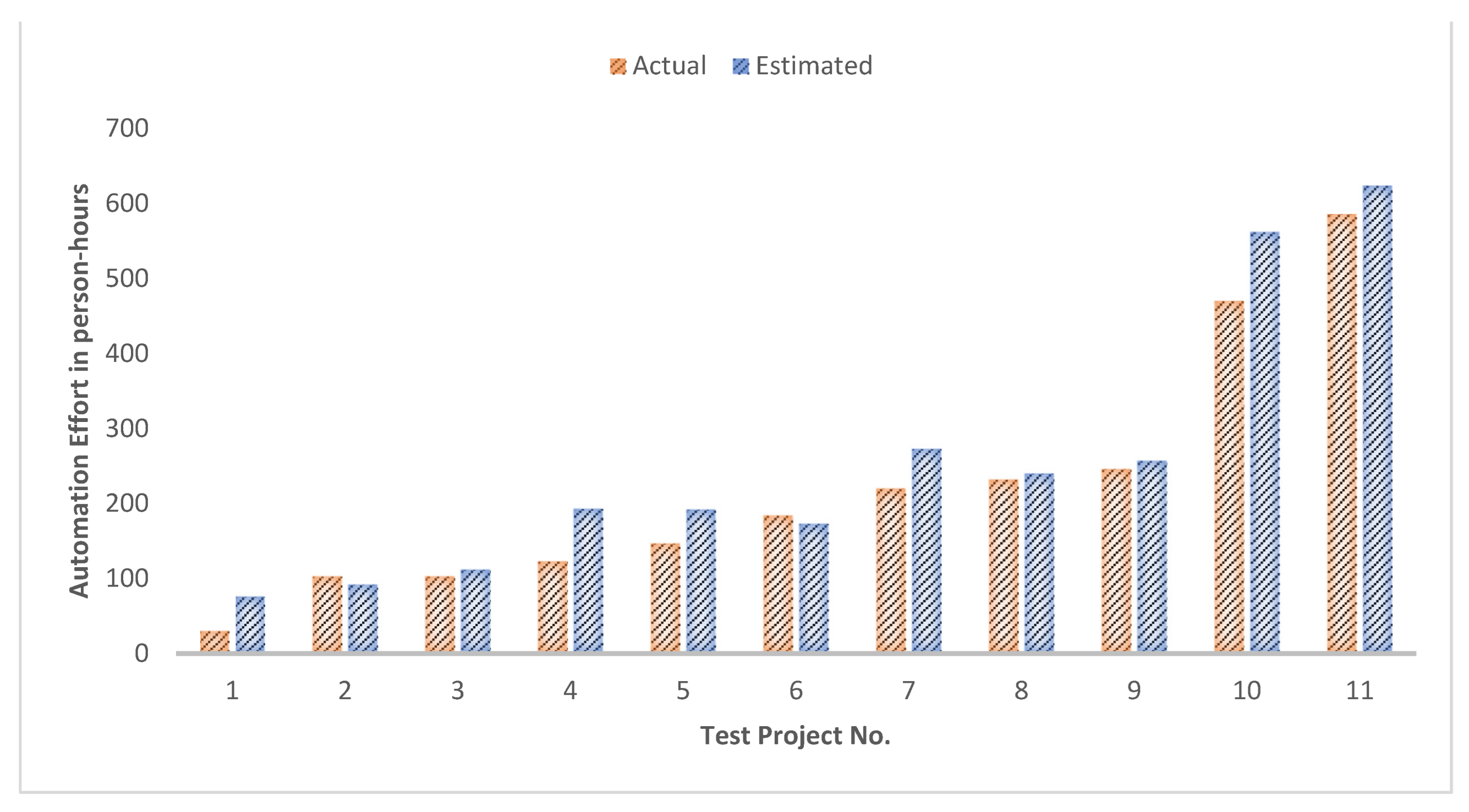
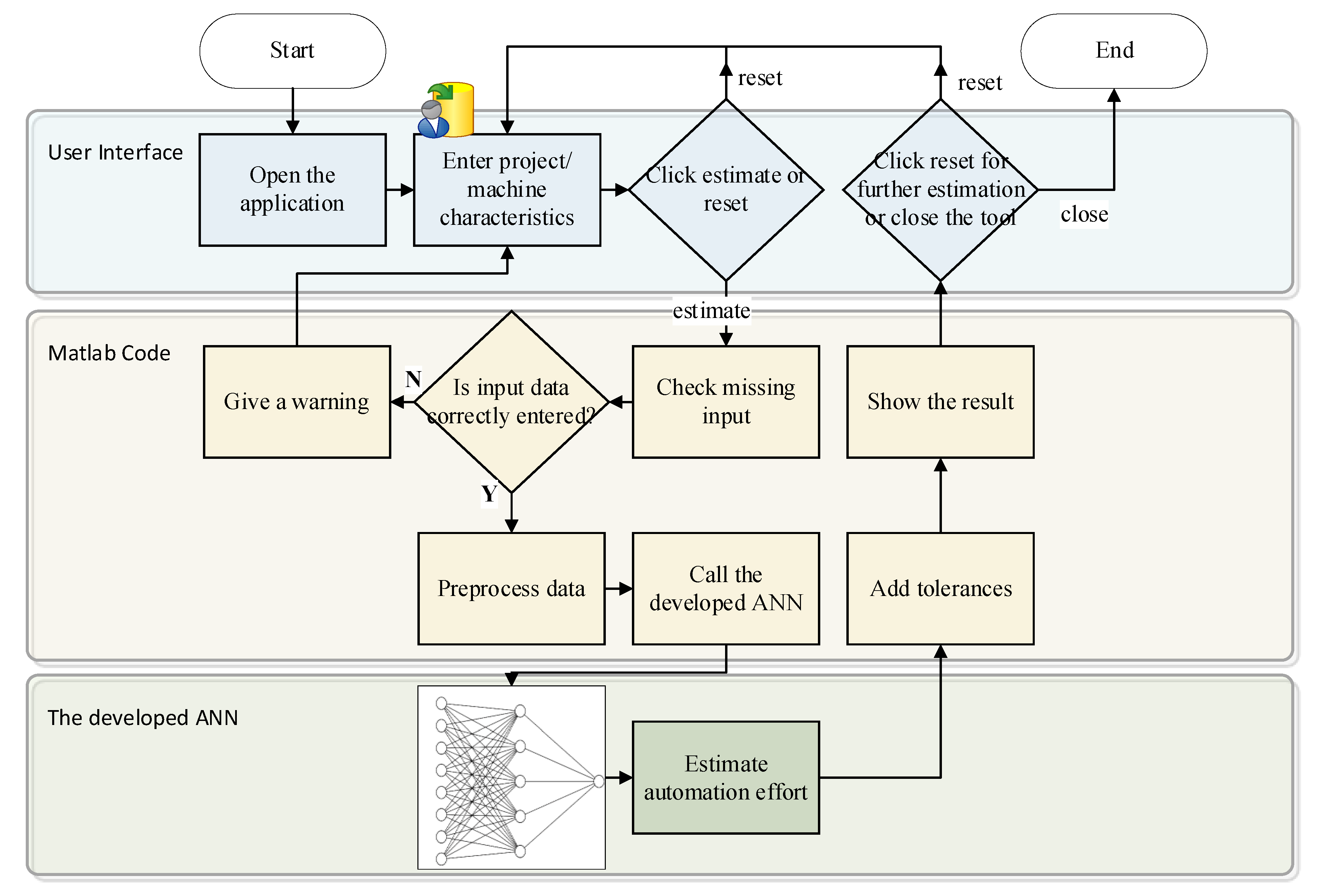
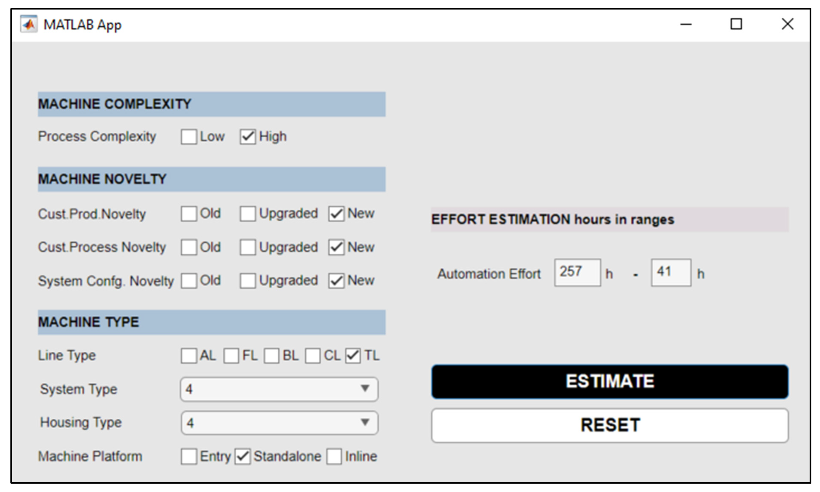
4.2. The ANN-Based Estimation Tool for Automation Effort of Machine Development Project
5. Conclusions
Author Contributions
Funding
Data Availability Statement
Conflicts of Interest
Abbreviations
| AHP | Analytic hierarchy process |
| ANN | Artificial neural network |
| BO | Bayesian optimization |
| COCOMO | Constructive cost model |
| DLNN | Deep learning neural networks |
| FFNN | Feed-forward neural network |
| GD | Gradient descent |
| GRNN | General regression neural network |
| HL | Hidden layer |
| LOC | Lines of code |
| ML | Machine learning |
| MLP | Multilayer perceptron |
| MMRE | Mean magnitude of relative errors |
| MRE | Magnitude of relative errors |
| MSE | Mean squared errors |
| NCA | Neighborhood component analysis |
| PRED | Prediction accuracy |
| RBFNN | Radial basis function neural network |
Appendix A. Experiments with the Chosen Hyperparameters for Performance Enhancement
| HN Size | Act. Func. for HL | Trial | R-Tra | R-Val | R-Test | MMRE-Tra | MMRE-Val | MMRE-Test | PRED(25) Tra | PRED(25) Val | PRED(25) Test | Best Epoch |
| 3 | logsig | 1 | 0.88 | 0.89 | 0.89 | 0.24 | 0.24 | 0.37 | 0.72 | 0.56 | 0.55 | 9 |
| 3 | logsig | 2 | 0.83 | 0.72 | 0.75 | 0.32 | 0.26 | 0.49 | 0.53 | 0.56 | 0.55 | 4 |
| 3 | logsig | 3 | 0.84 | 0.93 | 0.82 | 0.28 | 0.23 | 0.36 | 0.67 | 0.56 | 0.55 | 11 |
| 3 | logsig | 4 | 0.87 | 0.63 | 0.86 | 0.27 | 0.38 | 0.50 | 0.67 | 0.56 | 0.64 | 9 |
| 3 | logsig | 5 | 0.82 | 0.71 | 0.89 | 0.31 | 0.28 | 0.40 | 0.51 | 0.56 | 0.64 | 4 |
| 4 | logsig | 1 | 0.93 | 0.88 | 0.90 | 0.20 | 0.25 | 0.37 | 0.65 | 0.56 | 0.64 | 13 |
| 4 | logsig | 2 | 0.88 | 0.90 | 0.91 | 0.26 | 0.27 | 0.38 | 0.65 | 0.44 | 0.64 | 11 |
| 4 | logsig | 3 | 0.82 | 0.82 | 0.89 | 0.33 | 0.38 | 0.34 | 0.53 | 0.44 | 0.64 | 4 |
| 4 | logsig | 4 | 0.88 | 0.90 | 0.91 | 0.26 | 0.27 | 0.38 | 0.65 | 0.44 | 0.64 | 11 |
| 4 | logsig | 5 | 0.85 | 0.92 | 0.91 | 0.27 | 0.22 | 0.40 | 0.63 | 0.67 | 0.64 | 5 |
| 5 | logsig | 1 | 0.93 | 0.96 | 0.87 | 0.19 | 0.17 | 0.32 | 0.67 | 0.89 | 0.64 | 10 |
| 5 | logsig | 2 | 0.91 | 0.93 | 0.91 | 0.22 | 0.18 | 0.44 | 0.74 | 0.89 | 0.64 | 5 |
| 5 | logsig | 3 | 0.92 | 0.94 | 0.91 | 0.21 | 0.15 | 0.33 | 0.70 | 0.89 | 0.64 | 10 |
| 5 | logsig | 4 | 0.95 | 0.94 | 0.94 | 0.15 | 0.13 | 0.30 | 0.83 | 0.89 | 0.73 | 16 |
| 5 | logsig | 5 | 0.84 | 0.95 | 0.79 | 0.31 | 0.14 | 0.43 | 0.65 | 0.89 | 0.73 | 6 |
| 6 | logsig | 1 | 0.86 | 0.75 | 0.91 | 0.29 | 0.42 | 0.40 | 0.56 | 0.56 | 0.55 | 4 |
| 6 | logsig | 2 | 0.89 | 0.60 | 0.86 | 0.25 | 0.44 | 0.41 | 0.69 | 0.56 | 0.55 | 8 |
| 6 | logsig | 3 | 0.87 | 0.75 | 0.91 | 0.28 | 0.33 | 0.43 | 0.57 | 0.67 | 0.55 | 5 |
| 6 | logsig | 4 | 0.90 | 0.65 | 0.91 | 0.24 | 0.50 | 0.39 | 0.69 | 0.56 | 0.64 | 5 |
| 6 | logsig | 5 | 0.87 | 0.85 | 0.77 | 0.25 | 0.31 | 0.49 | 0.67 | 0.56 | 0.64 | 6 |
| 4 | tansig | 1 | 0.82 | 0.95 | 0.79 | 0.31 | 0.19 | 0.46 | 0.62 | 0.78 | 0.64 | 6 |
| 4 | tansig | 2 | 0.84 | 0.93 | 0.82 | 0.29 | 0.18 | 0.51 | 0.63 | 0.78 | 0.64 | 5 |
| 4 | tansig | 3 | 0.88 | 0.95 | 0.87 | 0.24 | 0.20 | 0.41 | 0.65 | 0.78 | 0.73 | 7 |
| 4 | tansig | 4 | 0.83 | 0.93 | 0.84 | 0.30 | 0.20 | 0.48 | 0.65 | 0.67 | 0.73 | 5 |
| 4 | tansig | 5 | 0.92 | 0.86 | 0.87 | 0.21 | 0.26 | 0.44 | 0.73 | 0.67 | 0.73 | 10 |
| 6 | tansig | 1 | 0.89 | 0.80 | 0.90 | 0.27 | 0.26 | 0.42 | 0.59 | 0.78 | 0.55 | 6 |
| 6 | tansig | 2 | 0.93 | 0.91 | 0.76 | 0.18 | 0.34 | 0.45 | 0.74 | 0.56 | 0.55 | 16 |
| 6 | tansig | 3 | 0.86 | 0.73 | 0.90 | 0.28 | 0.36 | 0.41 | 0.57 | 0.56 | 0.55 | 5 |
| 6 | tansig | 4 | 0.90 | 0.94 | 0.90 | 0.23 | 0.20 | 0.33 | 0.65 | 0.56 | 0.55 | 10 |
| 6 | tansig | 5 | 0.86 | 0.84 | 0.75 | 0.28 | 0.30 | 0.47 | 0.62 | 0.44 | 0.64 | 5 |
References
- Hameed, S.; Elsheikh, Y.; Azzeh, M. An optimized case-based software project effort estimation using genetic algorithm. Inf. Softw. Technol. 2023, 153, 107088. [Google Scholar] [CrossRef]
- Usman, M.; Britto, R.; Damm, L.O.; Börstler, J. Effort estimation in large-scale software development: An industrial case study. Inf. Softw. Technol. 2018, 99, 21–40. [Google Scholar] [CrossRef]
- Monika; Sangwan, O.P. Software effort estimation using machine learning techniques. In Proceedings of the 7th International Conference on Cloud Computing, Data Science & Engineering–Confluence, Noida, India, 12–13 January 2017. [Google Scholar] [CrossRef]
- Jørgensen, M.; Sjøberg, D.I.K. The impact of customer expectation on software development effort estimates. Int. J. Proj. Manag. 2004, 22, 317–325. [Google Scholar] [CrossRef]
- Carvalho, H.D.P.; Fagundes, R.; Santos, W. Extreme learning machine applied to software development effort estimation. IEEE Access 2021, 9, 92676–92687. [Google Scholar] [CrossRef]
- Prater, J.; Kirytopoulos, K.; Ma, T. Optimism bias within the project management context. Int. J. Manag. Proj. Bus. 2017, 10, 370–385. [Google Scholar] [CrossRef]
- Nassif, A.B.; Ho, D.; Capretz, L.F. Towards an early software estimation using log-linear regression and a multilayer perceptron model. J. Syst. Softw. 2013, 86, 144–160. [Google Scholar] [CrossRef]
- Tronto, I.F.B.; Silva, J.D.S.; Sant’Anna, N. An investigation of artificial neural networks based prediction systems in software project management. J. Syst. Softw. 2008, 81, 356–367. [Google Scholar] [CrossRef]
- Pospieszny, P.; Czarnacka-Chrobot, B.; Kobylinski, A. An effective approach for software project effort and duration estimation with machine learning algorithms. J. Syst. Softw. 2018, 137, 184–196. [Google Scholar] [CrossRef]
- López-Martín, C.; Chavoya, A.; Meda-Campaña, M.E. Software development effort estimation in academic environments applying a general regression neural network involving size and people factors. In Proceedings of the Pattern Recognition, 3rd Mexican Conference, MCPR, Cancun, Mexico, 29 June–2 July 2011; pp. 269–277. [Google Scholar] [CrossRef]
- Koch, S.; Mitlöhrer, J. Software project effort estimation with voting rules. Decis. Support Syst. 2009, 46, 895–901. [Google Scholar] [CrossRef]
- Arora, S.; Mishra, N. Software cost estimation using artificial neural network. Adv. Intell. Syst. Comput. 2018, 584, 51–58. [Google Scholar] [CrossRef]
- Heiat, A. Comparison of artificial neural network and regression models for estimating software development effort. Inf. Softw. Technol. 2002, 44, 911–922. [Google Scholar] [CrossRef]
- Bashir, H.A.; Thomson, V. Estimating design effort for GE hydro projects. Comput. Ind. Eng. 2004, 45, 195–204. [Google Scholar] [CrossRef]
- Yurt, Z.O.; Iyigun, C.; Bakal, P. Engineering effort estimation for product development projects. In Proceedings of the IEEE International Conference on Industrial Engineering and Engineering Management, Macao, China, 15–18 December 2019. [Google Scholar] [CrossRef]
- Ali, A.; Gravino, C.A. systematic literature review of software effort prediction using machine learning methods. J. Softw. Evol. Process 2019, 31, 1–25. [Google Scholar] [CrossRef]
- Dave, V.S.; Dutta, D.M.K. Application of Feed-Forward Neural Network in Estimation of Software Effort. IJCA Int. Symp. Devices MEMS Intell. Syst. Commun. 2011, 5, 5–9. [Google Scholar]
- Park, H.; Baek, S. An empirical validation of a neural network model for software effort estimation. Expert Syst. Appl. 2008, 35, 929–937. [Google Scholar] [CrossRef]
- Attarzadeh, I.; Ow, S.H. Software development cost and time forecasting using a high performance artificial neural network model. In Proceedings of the Intelligent Computing and Information Science, International Conference, Part I, Chongqing, China, 8–9 January 2011; pp. 18–26. [Google Scholar] [CrossRef]
- Rankovic, N.; Rankovic, D.; Ivanovic, M.; Lazic, L. Improved effort and cost estimation model using artificial neural networks and taguchi method with different activation functions. Entropy 2021, 23, 854. [Google Scholar] [CrossRef]
- Rijwani, P.; Jain, S. Enhanced software effort estimation using multi layered feed forward artificial neural network technique. Procedia Comput. Sci. 2016, 89, 307–312. [Google Scholar] [CrossRef]
- Attarzadeh, I.; Mehranzadeh, A.; Barati, A. Proposing an enhanced artificial neural network prediction model to improve the accuracy in software effort estimation. In Proceedings of the International Conference on Computational Intelligence, Communication Systems and Networks, Phuket, Thailand, 24–26 July 2012; pp. 167–172. [Google Scholar] [CrossRef]
- Predescu, E.F.; Stefan, A.; Zaharia, A.V. Software effort estimation using multilayer perceptron and long short term memory. Inform. Econ. 2019, 23, 76–87. [Google Scholar] [CrossRef]
- Jaifer, R.; Beauregard, Y.; Bhuiyan, N. New Framework for effort and time drivers in aerospace product development projects. Eng. Manag. J. 2021, 33, 76–95. [Google Scholar] [CrossRef]
- Arundacahawat, P.; Roy, R.; Al-Ashaab, A. An analogy-based estimation framework for design rework efforts. J. Intell. Manuf. 2013, 24, 625–639. [Google Scholar] [CrossRef]
- Pollmanns, J.; Hohnen, T.; Feldhusen, J. An information model of the design process for the estimation of product development effort. In Proceedings of the 23rd CIRP Design Conference, Smart Product Engineering, Bochum, Germany, 11–13 March 2013; pp. 885–894. [Google Scholar] [CrossRef]
- Salam, A.; Bhuiyan, N.F.; Gouw, G.J.; Raza, S.A. Estimating design effort in product development: A case study at Pratt & Whitney Canada. In Proceedings of the International Conference on Industrial Engineering and Engineering Management, Singapore, 2–4 December 2007. [Google Scholar] [CrossRef]
- Singh, A.J.; Kumar, M. Comparative analysis on prediction of software effort estimation using machine learning techniques. In Proceedings of the 1st International Conference on Intelligent Communication and Computational Research (ICICCR-2020), Delhi, India, 20–22 February 2020. [Google Scholar] [CrossRef]
- Goyal, S.; Bhatia, P.K. Feature selection technique for effective software effort estimation using multi-layer perceptrons. Emerging trends in information technology. In ICETIT 2019, Emerging Trends in Information Technology; Springer: Berlin/Heidelberg, Germany, 2020; pp. 183–194. [Google Scholar] [CrossRef]
- Azzeh, M.; Nassif, A.B. A hybrid model for estimating software project effort from Use Case Points. Appl. Soft Comput. J. 2016, 49, 981–989. [Google Scholar] [CrossRef]
- Pandey, M.; Litoriya, R.; Pandey, P. Validation of existing software effort estimation techniques in context with mobile software applications. Wirel. Pers. Commun. 2020, 110, 1659–1677. [Google Scholar] [CrossRef]
- Holzmann, V.; Zitter, D.; Peshkess, S. The expectations of project managers from artificial intelligence: A Delphi Study. Proj. Manag. J. 2022, 53, 438–455. [Google Scholar] [CrossRef]
- Haykin, S.S. Neural Networks and Learning Machines, 3rd ed.; Prentice Hall/Pearson: London, UK, 2008. [Google Scholar]
- Kumar, P.S.; Behera, H.S.; Kumari, A.K.; Nayak, J.; Naik, B. Advancement from neural networks to deep learning in software effort estimation: Perspective of two decades. Comput. Sci. Rev. 2020, 38, 100288. [Google Scholar] [CrossRef]
- Rao, P.S.; Kumar, R.K. Software effort estimation through a generalized regression neural network. In Proceedings of the Emerging ICT for Bridging the Future, Advances in Intelligent Systems and Computing, the 49th Annual Convention of the Computer Society of India, Hyderabad, India, 11–15 December 2015; Volume 337, pp. 19–30. [Google Scholar] [CrossRef]
- Makarova, A.; Shen, H.; Perrone, V.; Klein, A.; Faddoul, J.B.; Krause, A.; Seeger, M.; Archambeau, C. Overfitting in Bayesian optimization: An empirical study and early-stopping solution. In Proceedings of the 2nd Workshop on Neural Architecture Search at ICLR, Online, 7 May 2021. [Google Scholar]
- Jun, E.S.; Lee, J.K. Quasi-optimal case-selective neural network model for software effort estimation. Expert Syst. Appl. 2001, 21, 1–14. [Google Scholar]
- Pai, D.R.; McFall, K.S.; Subramanian, G.H. Software effort estimation using a neural network ensemble. J. Comput. Inf. Syst. 2013, 53, 49–58. [Google Scholar] [CrossRef]
- Hutter, F.; Kotthoff, J.; Vanschoren, J. Automated Machine Learning: Methods, Systems, Challenges; Springer: Berlin/Heidelberg, Germany, 2019; Chapter 1. [Google Scholar] [CrossRef]
- Zheng, A. Evaluating Machine Learning Models: A Beginner’s Guide To Key Concepts and Pitfalls, 1st ed.; O’Reilly Media, Inc.: Sebastopol, CA, USA, 2015; pp. 27–37. [Google Scholar]
- Snoek, J.; Larochelle, H.; Adams, R.P. Practical Bayesian optimization of machine learning algorithms. arXiv 2012. [Google Scholar] [CrossRef]
- Nguyen, V.; Gupta, S.; Rana, S.; Li, C.; Venkatesh, S. Regret for expected improvement over the best-observed value and stopping condition. In Proceedings of the Ninth Asian Conference on Machine Learning, PMLR, Seoul, Repubulic of Korea, 15–17 November 2017; Volume 77, pp. 279–294. [Google Scholar]
- Zhao, Y.; Li, Y.; Feng, C.; Gong, C.; Tan, H. Early warning of systemic financial risk of local systemic financial risk of local government implicit debt based on BP neural network models. Systems 2022, 10, 207. [Google Scholar] [CrossRef]
- Johansson, E.M.; Dowla, F.U.; Goodman, D.M. Backpropagation learning for multilayer feed-forward neural networks using the conjugate gradient method. Int. J. Neural Syst. 1992, 4, 291–301. [Google Scholar] [CrossRef]
- Reddy, P.V.G.D.; Sudha, K.R.; Rama, S.P.; Ramesh, S.N.S.V.S.C. Software effort estimation using radial basis and generalized regression neural network. J. Comput. 2010, 2, 87–92. [Google Scholar] [CrossRef]
- Kalichanin-Balich, I.; Lopez-Martin, C. Applying a feedforward neural network for predicting software development effort of short-scale projects. In Proceedings of the 8th ACIS International Conference on Software Engineering Research, Management and Applications, Montreal, QC, Canada, 24–26 May 2010. [Google Scholar] [CrossRef]
- Sharma, S.; Vijayvargiya, S. An optimized neuro-fuzzy network for software project effort estimation. IETE J. Res. 2022. [Google Scholar] [CrossRef]


| No. | Variable Name | Level | Role |
|---|---|---|---|
| 1 | Process complexity | 1: low, 2: high | Input |
| 2 | Customer product novelty | 1: no change, 2: upgraded, 3: new | Input |
| 3 | Customer process novelty | 1: no change, 2: upgraded, 3: new | Input |
| 4 | System configuration novelty | 1: no change, 2: upgraded, 3: new | Input |
| 5 | Machine function | Five categories regarding types of functions based on a machine’s primary function | Input |
| 6 | Machine main system size | Six categories | Input |
| 7 | Machine housing size | 1: No housing, 2: extra small, 3: small, 4: medium, 5: large, 6: extra large | Input |
| 8 | Machine line type | 1: entry, 2: standalone, 3: in-line | Input |
| 9 | Automation effort | Required effort for the automation phase of a machine development project | Output |
| Hyperparameters to be Optimized | Possible Values |
|---|---|
| The number of neurons at 1st HL | 2–8 |
| Activation function for 1st HL | tansig, logsig, purelin |
| Activation function for output layer | tansig, logsig, purelin |
| Iteration Number | Observed Objective | The Number of Hidden Neurons | Activation Function of the Hidden Layer | Activation Function of the Output Layer |
|---|---|---|---|---|
| 5 | 0.19756 | 6 | logsig | purelin |
| 6 | 0.19718 | 4 | logsig | purelin |
| 7 | 0.20445 | 5 | logsig | purelin |
| 8 | 0.19865 | 3 | logsig | purelin |
| 9 | 0.19934 | 4 | tansig | purelin |
| 10 | 0.20332 | 6 | tansig | purelin |
| MSElog | R-Value | MMRE | PRED(25) | |
|---|---|---|---|---|
| Training | 0.04 | 0.95 | 0.15 | 0.83 |
| Validation | 0.03 | 0.94 | 0.13 | 0.89 |
| Test | 0.11 | 0.94 | 0.30 | 0.73 |
| Year | Author(s) | Ref. | Method | Prediction Accuracy |
|---|---|---|---|---|
| 2002 | Heiat | [13] | RBFNN | MAPE: 31.96% |
| 2008 | Tronto et al. | [8] | MLP | MMRE: 41.53% |
| 2008 | Park and Baek | [18] | ANN | MRE: 59.40% |
| 2010 | Reddy, Sudha, Rama, Ramesh | [45] | RBFNN, GRNN | MMRE: 17.29%, 34.61% |
| 2010 | Kalichanin-Balich and Lopez-Martin | [46] | FFNN | MMER: 22% |
| 2011 | Lopez-Martin et al. | [10] | GRNN | MMER: 26% |
| 2011 | Attarzadeh and Ow | [19] | MLP | MMRE: 45%, PRED(25): 43.30% |
| 2012 | Attarzadeh et al. | [22] | FFNN | MMRE: 46%, PRED(25): 45.50% |
| 2013 | Nassif et al. | [7] | MLP | MMER: 40%, PRED(25): 45.70% |
| 2013 | Pai, McFall, Subramanian | [38] | MLP | MMRE: 59.30% |
| 2016 | Rijwani and Jain | [21] | FFNN | MMRE: 14.40% |
| 2018 | Pospieszny et al. | [9] | MLP | MMRE: 21%, PRED(25): 64.65%, MMER: 45% |
| 2020 | Goyal and Bhatia | [29] | FFNN | MMRE: 25.80%, R-value: 90% |
| 2020 | Pandey et al. | [31] | MLP | MMRE: 24%, PRED(25): 42% |
| 2021 | Rankovic et al. | [20] | MFFN with the Taguchi method | MMRE: 16.10%, PRED(25): 50% |
| 2021 | Carvalho, Fagundes, Santos | [5] | MLP, Extreme Learning Machine | MMRE: 42%, 18% |
| 2022 | Sharma and Vijayvargiya | [47] | Wavelet ANN, Genetic Elephant Herding Optimization-based Neuro-Fuzzy Network | MMRE: 22.08%, 16.70% |
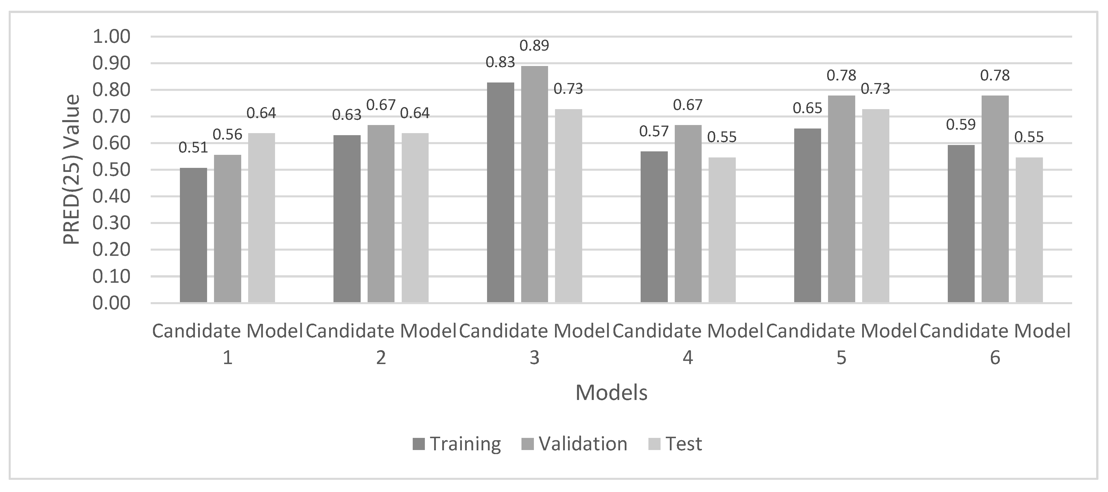
| The Number of Hidden Neurons | Activation Function | Experiment No. (Appendix A) | Candidate Model No. | MMRE | PRED(0.25) | ||||
|---|---|---|---|---|---|---|---|---|---|
| Tra | Val | Test | Tra | Val | Test | ||||
| 3 | logsig | 5 | 1 | 0.31 | 0.28 | 0.40 | 0.51 | 0.56 | 0.64 |
| 4 | logsig | 5 | 2 | 0.27 | 0.22 | 0.40 | 0.63 | 0.67 | 0.64 |
| 5 | logsig | 4 | 3 | 0.15 | 0.13 | 0.30 | 0.83 | 0.89 | 0.73 |
| 6 | logsig | 3 | 4 | 0.28 | 0.33 | 0.43 | 0.57 | 0.67 | 0.55 |
| 4 | tansig | 3 | 5 | 0.24 | 0.20 | 0.41 | 0.65 | 0.78 | 0.73 |
| 6 | tansig | 1 | 6 | 0.27 | 0.26 | 0.42 | 0.59 | 0.78 | 0.55 |
| MMRE | PRED(25) | MAE | RMSE | |||||
|---|---|---|---|---|---|---|---|---|
| MLR | Proposed ANN | MLR | Proposed ANN | MLR | Proposed ANN | MLR | Proposed ANN | |
| Training | 0.54 | 0.15 | 0.32 | 0.83 | 94.54 | 32.77 | 128.09 | 52.79 |
| Validation | 0.27 | 0.13 | 0.78 | 0.89 | 57.17 | 44.25 | 67.17 | 62.85 |
| Test | 0.92 | 0.30 | 0.27 | 0.73 | 96.82 | 35.89 | 115.33 | 45.03 |
| No. | Input Name | Selected Value | No. | Input Name | Selected Value |
|---|---|---|---|---|---|
| 1 | Process complexity | High | 5 | Machine function | Test machine |
| 2 | Customer product novelty | New | 6 | Machine main system size | Medium |
| 3 | Customer process novelty | New | 7 | Machine housing size | Medium |
| 4 | System configuration novelty | New | 8 | Machine line type | Standalone |
Disclaimer/Publisher’s Note: The statements, opinions and data contained in all publications are solely those of the individual author(s) and contributor(s) and not of MDPI and/or the editor(s). MDPI and/or the editor(s) disclaim responsibility for any injury to people or property resulting from any ideas, methods, instructions or products referred to in the content. |
© 2023 by the authors. Licensee MDPI, Basel, Switzerland. This article is an open access article distributed under the terms and conditions of the Creative Commons Attribution (CC BY) license (https://creativecommons.org/licenses/by/4.0/).
Share and Cite
Şengüneş, B.; Öztürk, N. An Artificial Neural Network Model for Project Effort Estimation. Systems 2023, 11, 91. https://doi.org/10.3390/systems11020091
Şengüneş B, Öztürk N. An Artificial Neural Network Model for Project Effort Estimation. Systems. 2023; 11(2):91. https://doi.org/10.3390/systems11020091
Chicago/Turabian StyleŞengüneş, Burcu, and Nursel Öztürk. 2023. "An Artificial Neural Network Model for Project Effort Estimation" Systems 11, no. 2: 91. https://doi.org/10.3390/systems11020091
APA StyleŞengüneş, B., & Öztürk, N. (2023). An Artificial Neural Network Model for Project Effort Estimation. Systems, 11(2), 91. https://doi.org/10.3390/systems11020091