Article

Developing a Stochastic Two-Tier Architecture for Modelling Last-Mile Delivery and Implementing in Discrete-Event Simulation

Department of Mechanical Engineering, University of Canterbury, Kirkwood Ave, Christchurch 8140, New Zealand
*
Authors to whom correspondence should be addressed.
Systems 2022, 10(6), 214; https://doi.org/10.3390/systems10060214
Submission received: 8 September 2022 / Revised: 30 October 2022 / Accepted: 8 November 2022 / Published: 10 November 2022

Abstract

:
Modelling freight logistics is challenging due to the variable consignments and diverse customers. Discrete-event Simulation (DES) is an approach that can model freight logistics and incorporate stochastic events. However, the flexible delivery routes of Pickup and Delivery (PUD) are still problematic to simulate. This research aims to develop last-mile delivery architecture in DES and evaluate the credibility of the model. A two-tier architecture was proposed and integrated with a DES model to simulate freight operations. The geographic foundation of the model was determined using Geographic Information Systems (GIS), including identifying customer locations, finding cluster centres, and implementing Travelling Salesman Problem (TSP) simulation. This complex model was simplified to the two-tier architecture with stochastic distances, which is more amenable to DES models. The model was validated with truck GPS data. The originality of the work is the development of a novel and simple methodology for developing a logistics model for highly variable last-mile delivery.

1. Introduction

Freight transportation plays an important role in supporting economic growth [1]. It is required to transport goods from the origin to the destination, including trade, logistics and transportation, including linehaul and urban pickup and delivery (PUD). The operations are highly complex, especially in transport activities, because variable customer addresses and freight consolidation affect route planning [2]. These factors cause the delivery route to be difficult to model. In New Zealand (NZ), the country under examination, the New Zealand Business Council estimates freight will increase by 75% in the next 30 years [3], and this is broadly consistent with elsewhere in the world. Hence there is a need for optimization and continuous improvement regarding logistics efficiency [4]. In turn, this requires modelling and simulation.
Computer simulation techniques are primarily discrete-event simulation (DES), and agent-based modelling (ABM). DES readily accommodates stochastic variability, and it also has the means to model conditional events [5]. It has been widely applied to logistics as well as plant layout and service queuing problems [6,7]. ABM has the advantage of more easily accommodating the choices of individual agents and including their behaviours and interactions. Examples of applications to logistics are the agents being trucks to optimise freight distribution [8] and being locations to solve routing problems [9]. Another avenue of simulation is provided by geographic information systems (GIS). While DES and ABM primarily operate in the time domain, GIS is in the spatial domain. Typical logistics applications are to determine routes (and hence distance) between physical addresses [10], with the travel time a secondary determination by introducing speeds. GIS requires precise identification of the addresses, and hence offers a specific rather than generalised simulation method. The present paper focuses on DES as applied to freight last-mile delivery.
However, the delivery route is challenging to incorporate in DES models due to the dynamic nature of operations, especially the daily variability of consignments and the variability in route [11,12]. An intersection-based DES model has been developed [13], but it is difficult to apply to changeable conditions. This is where models with simpler architectures can be advantageous, especially from an operational perspective.
The motivation of this work is to develop an architecture to represent last-mile delivery suitable for integration with stochastic models. The present paper shows how clustering may be applied to develop a two-tier architecture capable of representing the complexity of last-mile delivery routes for a variable number and address-set of consignments. A case study is presented using representative industry data. The method is demonstrated by a case study.
The paper is structured as follows: Section 2 is a literature review of last-mile delivery modelling methods. Section 3 introduces the proposed two-tier delivery model. Section 4 describes the implementation of the proposed method through a case study for real freight operations.

2. Literature Review

Last-mile delivery models may be an approach in three main ways: mathematical models, computer simulation models, and GIS models. These are briefly reviewed below.

2.1. Mathematical Modelling of Vehicle Routing Problems (VRP)

Freight last-mile delivery is highly variable and requires flexible route planning, because of daily variability in customers being served and freight volume. Conventional approaches to modelling last-mile delivery have primarily taken the consolidation perspective whereby consignments are aggregated to delivery runs within geographic territories. This results in the need to solve vehicle routing problems (VPR). There are various forms of VPR, including node routing problem (NRP) [14,15], travelling salesman problem (TSP) [16,17,18], arc routing problem (ARP) [19,20,21], rural postman problem (RPP) [22,23] and Chinese postman problem (CPP) [24,25,26]. All these methods apply a mathematical optimisation to find the most efficient route given the constraints applied.
There are innovative methods to simulate last-mile delivery, including agent-based models [27], system dynamics models [28], the fuzzy analytic hierarchy process model [29], Petri net models [30], crowd shipping models [31], Hamiltonian cycle model [32], continuous approximation models [33] and the dynamic traffic simulation [34]. Applications of mathematical route models to freight last-mile delivery are numerous. However, there are limitations in these models. The simplifications in the models make it difficult to include all operational constraints [13]. These methods may have some but limited ability to represent stochastic variability because of the complexity of metaheuristic calculations [35,36]. However, they fare poorly with the epistemic uncertainty that arises from variability in simulating real-life problems. Many of these methods do not generalise well—they are specific solutions for a given set of customer addresses, and for a different set, the model has to be re-run in its entirety. This limitation makes it difficult to apply in real operational situations where real-time modelling is appreciated.

2.2. Computer Simulation

Computer simulation techniques include discrete-event simulation (DES), agent-based simulation (ABS) and system dynamics (SD). Compared with conventional mathematical models, simulation models tend to describe systems and measure system performance [37]. DES is a versatile simulation technique to solve practical problems [38]. It imitates systems with predefined architecture and resources. The process is divided into sequential discrete events. This attribute reduces the complexity of computations on constraints and allows probability distributions to be incorporated with the Monte Carlo sampling method. Examples of DES applications in logistics include rail freight models [39], multimodal transport [40], underground logistics transportation [41], container port operations [42], logistics planning [43] and fleet management [44,45].
Perhaps unexpectedly, there is a scarcity of literature on the application of computer modelling for freight last-mile delivery. For an exception, see an agent-based model which was applied to evaluate delivery cutoff times (the responsiveness question) but not distances [46].
As applied to modelling freight last-mile delivery, all the computer simulation methods offer the positive features of coping with stochastic parameters, and can represent complex systems, including decisions, specifically model resource utilisation & report on productivity metrics. The ABS methods have the further advantage of being to represent individual behaviour, such as specific route choices of vehicles. Agency is also possible with DES, although it requires more effort to model the necessary decision blocks.
Disadvantages of computer simulation as applied to freight last-mile delivery are the greater effort to create the model, and the difficulty of representing specific routes. Also, the models are descriptive rather than the basis for optimisation. Another challenge is the difficulty in the validation of the model, and this becomes increasingly difficult as the model becomes more complex. The model requires prior assumptions about the architecture of the problem (the underlying structure of the decision problem), which tend to be obscured within the computer models. Furthermore, supply chain models require many assumptions, and it is difficult to obtain accurate estimates for real-world situations [47].
The underlying problem is that optimisation of final mile routes is a hard combinatorial problem that these types of simulation cannot solve or even represent.

2.3. Geographic Information System

GIS can manage, display and analyse large spatial data sets. It has also been used to model last-mile delivery, and has some attributes that make it very different to the mathematical models. In particular, GIS is good at representing addresses and road routes, including road information and traffic conditions (including congestion, and time-of-day variability therein), and road suitability for freight trucks. This can make for powerful models, and indeed GIS may be used to solve TSP problems. Applications of GIS to logistics and transportation generally include formulation of future transportation plans [48], multimodal freight [49], routes for forest firefighters [50], oil and gas transportation [51] and e-commerce logistics distribution [52].
GIS has benefits in implementing simple TSP simulations. It can accurately identify locations and incorporate geographical data. Therefore, the route results can be an authentic representation of real truck routes selected by experienced drivers.
An application to last-mile delivery and PUD is evident in [13], where GIS was used to find the routes for two models (a simple suburb model and an intersection-based model), which were subsequently represented in DES with predefined routing decisions and stochastic simulation.
Some comparable work is available on the use of GIS to determine routes for waste collection [53,54,55,56]. However, waste collection is a different and simpler problem: in waste collection, the need is to determine a route that takes every street, and once determined the truck always follows the same route. In contrast, last-mile delivery does not require every street to be covered every day, and new optimisation is needed every day.
Consequently, although GIS has the advantage of simulating freight delivery routes, a general limitation of GIS as regards modelling logistics operations is that it mainly focuses on standalone cases. In an operational situation with high daily variability in customers, the model has to be re-run for each situation. Also, GIS is challenging to include freight operations such as queuing models and the freight consolidation process. It is possible to integrate ad-hoc plug-ins with GIS to extend the functionality, but the existing applications are limited.

2.4. Gaps in the Modelling of Freight Last-Mile Delivery

The integration of mathematical, simulation and GIS models has been shown in recent literature. GIS was utilised to obtain natural hazard data and support mathematical model development for optimising post-disaster relief distribution and network restoration [57]. GIS can also support discrete-event model development, which has been presented in [13]. In addition, a Monte Carlo simulation has been combined with a multi-objective model to analyse an electronic reverse logistics network with stochasticity [58]. It is also possible to incorporate simulation models into mathematical models. A DES model was integrated with a mixed-integer programming model to allocate vessels [59]. The mathematical model assisted in optimizing the process.
There are extensive works of literature on clustering design approaches and route approximation models. The works of literature are summarised in Table 1. However, these models rarely incorporate a logistics model to represent realistic operations and address a large number of stochastic variables. DES has the strength to measure operational performance, and compare different scenarios [60], but struggles with the optimisation of final mile routes that change on a daily basis. Therefore, there is a gap in developing an architecture to represent last-mile delivery suitable for integration with stochastic models.

3. Methodology

3.1. Research Objective

The objectives of this research were to find an architecture that can reflect the freight delivery route with high flexibility, suitable for incorporation into a DES model. This is worth attempting, for the benefit of being able to include stochastic elements in the model. DES models are relatively quick to implement in an operational sense, and have the potential to be aggregated into larger simulation models.

3.2. Approach

For logistics modelling, the delivery route is challenging to simulate in terms of travel distance and travel time. A two-tier architecture was developed to represent the delivery route and incorporate stochasticity for a concentrated cluster to estimate the travel distance. The accuracy of the architecture was validated by a case study. A freight logistics model was developed by DES and conducted in Arena® (version 16.00, Rockwell Automation, Milwaukee, WI, USA). ArcGIS Pro® (version 2.6.3, Esri, Redlands, CA, USA) was applied to find cluster centres, calculate distances and run TSP simulation. TSP simulation is generally used to find the optimal route by organising the sequence of customer locations. ArcGIS was used for TSP simulation because it can provide more accurate routes and distances in terms of customer locations and road information with the existing database.

3.2.1. Developing a Two-Tier Architecture

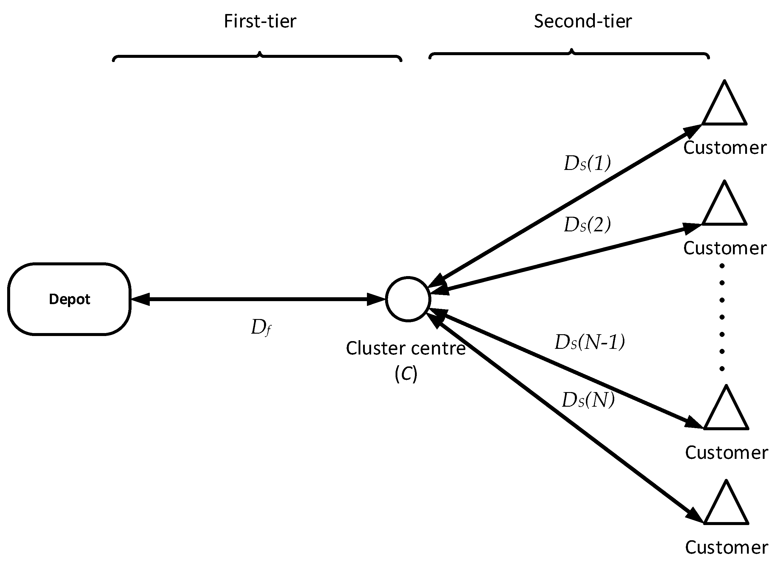
To simplify the delivery route and apply it to a DES model, the route was divided into two tiers, as Figure 1 shows, with the first tier from the depot to the cluster centre and the second tier from the cluster centre to each customer. Hence in this architecture, the first-tier distance is fixed, and the second-tier distance is stochastic since the customer location varies. All parameters for the architecture are calculated based on TSP results. Then the architecture is developed in a DES model accordingly. For N consignments, the estimated route distance is the sum of the first-tier distance and all second-tier distances. In practice, the truck does a tour and travels back to the depot at the end, rather than shuttling between the cluster centre and the customer addresses.
To obtain the first-tier distance ( D f ) , the cluster centre (C) should be determined first. There are several methods to find the cluster centre, including cluster mean centres and cluster median centres with data point attributes. The second-tier distance ( D s ) for each customer location is stochastic, which can be calculated by multiplying the Euclidean distance ( D e ) from the cluster centre to the customer locations and a factor R. The total travel distance ( D t o t a l ) for the journey is:
D t o t a l = 2 D f + D s ( i )   i   N
D s   ( i ) = R D e ( i )   i   N
The factor R adjusts   D e and hence D s , so D t o t a l is close to the real route distance.

3.2.2. Determining R

The first-tier distance ( D f ) can be calculated once the cluster centre (C) is defined. The R value is comparatively difficult to obtain, which determines the second-tier distance ( D s ).
The intention of introducing R is to adjust the total second-tier distance and approach to the real delivery distance. To acquire the R value, TSP simulation is a technique to simulate delivery routes and obtain the total route distance ( D t ). Then the imaginary second-tier distance ( D m ) can be calculated by Equation (3) and one R value can be determined by Equation (4) regarding one TSP simulation.
D m = D t 2 D f
R = D m D s
The R values can be obtained through implementing TSP simulation with different customer locations.

3.2.3. Implementation Stages

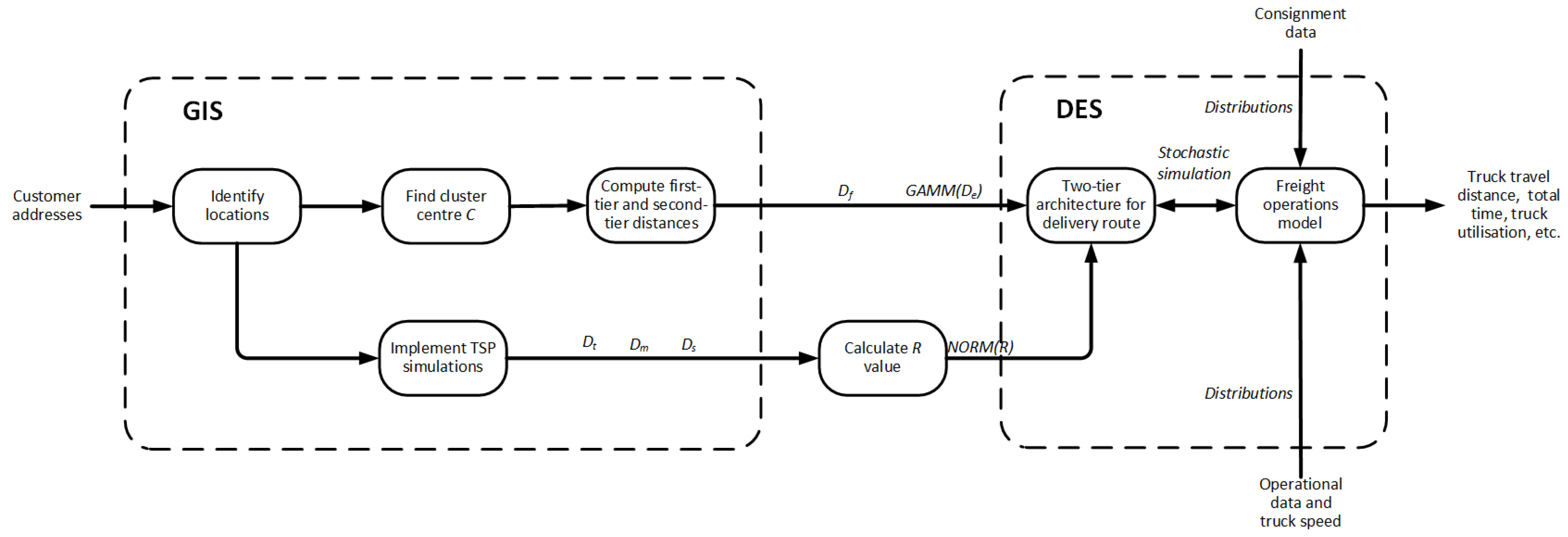
GIS was applied to develop the two-tier architecture, which is a part of the logistics model. The holistic logistics model was created by DES. The model development process is illustrated in Figure 2.
Step 1: Consignment data and truck GPS data were obtained from the industry. Operational data were manually recorded.
Step 2: Consignment data were input in ArcGIS and customer locations were identified. Different types of centres are mean and median, for the number of consignments, weight, and volume. The algorithms were the standard implementations in ArcGIS. The centre selected was the mean by consignments.
Step 3: The first-tier distance ( D f ) and the second-tier distances ( D e ) were computed in ArcGIS and the second distances were formed into a Gamma distribution.
Step 4: Random sets of addresses were generated to simulate different delivery routes. The consignment range considered is from 10 to 15, which is common for daily delivery. Hence, cases for n = 10 and n = 15 consignments were analysed. There was a total of ten ensembles for each. The corresponding addresses were input in ArcGIS. TSP simulations were conducted in ArcGIS to find each delivery tour and obtain ( D t ). These tours were not from the cluster centre, but from the depot, and were believed to closely represent real routes [13].
Step 5: The R values were calculated by D m and D s and formed into Normal distributions for each consignment number.
Step 6: The DES model for freight logistics was created in Arena by incorporating the two-tier architecture. Freight operations, including freight loading, unloading and consolidation were developed in the model, see Figure 3.
Step 7: Consignment data and operational data were formed into distributions and input into the DES model. The truck speed was calculated based on the GPS data.
Step 8: Stochastic simulation was conducted by the DES model. Results about truck travel distance, total time, truck utilisation and truckload were produced.

4. Results

4.1. Description of the Case Study

The specific case under investigation is freight delivery. The truck delivered freight consignments by a sequence in an intensive area. One-year consignment data and the truck GPS data were obtained from the industry partner. Data included customer address, freight attributes and truck speeds. Two cases were assumed, which are 10 delivery consignments (n = 10) and 15 delivery consignments (n = 15). Operations of freight delivery were observed by the first author. The freight loading time was recorded on-site and the unloading time was obtained from the GPS data. Operations were validated with the industry partner through face validation. Embedded communication was conducted to solicit tacit knowledge [12]. Key assumptions are shown in Table 2.

4.2. Determining the Parameters for Two-Tier Architecture

Suburbs with weight and volume less than 3% of the total were neglected to simplify the model. The driver’s main service areas are concentrated in Wigram and Sockburn. Therefore, addresses in Wigram and Sockburn were considered as one cluster. The proportion of consignment quantities, weight and volume for suburbs in Christchurch is shown in Table 3.
One-year consignment data were input in ArcGIS. The number of data points was 3195. Figure 4 exhibits hotspots of consignment data with attributes of the consignment number, weight and volume in ArcGIS. These hotspots were calculated based on the target features within Euclidean Distance [61].
All three hotspot maps show a similar distribution by different attributes. Therefore, the centre of the cluster can incorporate the feature of the number of consignments, consignment weight and volume in the two-tier architecture.
Individual customer locations are challenging to embody in logistics models. Therefore, clusters may be considered in models instead of specific locations. The principle of cluster analysis is to make the objects in the same cluster have the greatest possible similarity. Then a representative centre is applied to express the cluster [62]. Cluster centres and centroids have emerged in research, including wireless sensor networks [63], the internet of things [64], biological systems [65] and the global navigation satellite system [66].
Cluster centres are also defined in the K-means clustering algorithm. K-means clustering is based on the concept of dividing n points into k clusters, so that each point belongs to the cluster corresponding to the nearest centre [67]. Combined with the K-means clustering algorithm, GIS may be used to identify the peak travel of residents and hot spots for taxis [68]. K-means clustering was used to establish hot spots where road accidents occur [69]. Similarly, a modified clustering method (DP-Dip) has been used to estimate the centre of the cluster [70]. DP-Dip does not make any assumptions about the data distribution and only admits that each cluster has a unimodal distribution. This method adaptively splits some clusters according to their density.
The benefits of clustering are that it provides a simple representation of the problem, which may be used to infer structure in a wider data set of addresses. However, applications of clustering to last-mile delivery are scarce. Successful applications include food delivery [71]. Costs were estimated by K-means clustering for restaurants in a city. However, the difficulty with the clustering approach for logistics is the high degree to which the operation reality has been simplified. Therefore, a cluster model can represent an average operational day, but does not correspond to the operational reality for any one day. Also, vehicles do not actually travel backwards and forwards from a cluster centre, but rather have a delivery run. In situations where the delivery addresses have high day-to-day variability, clustering methods are inadequate because the need is to represent vehicle routing.
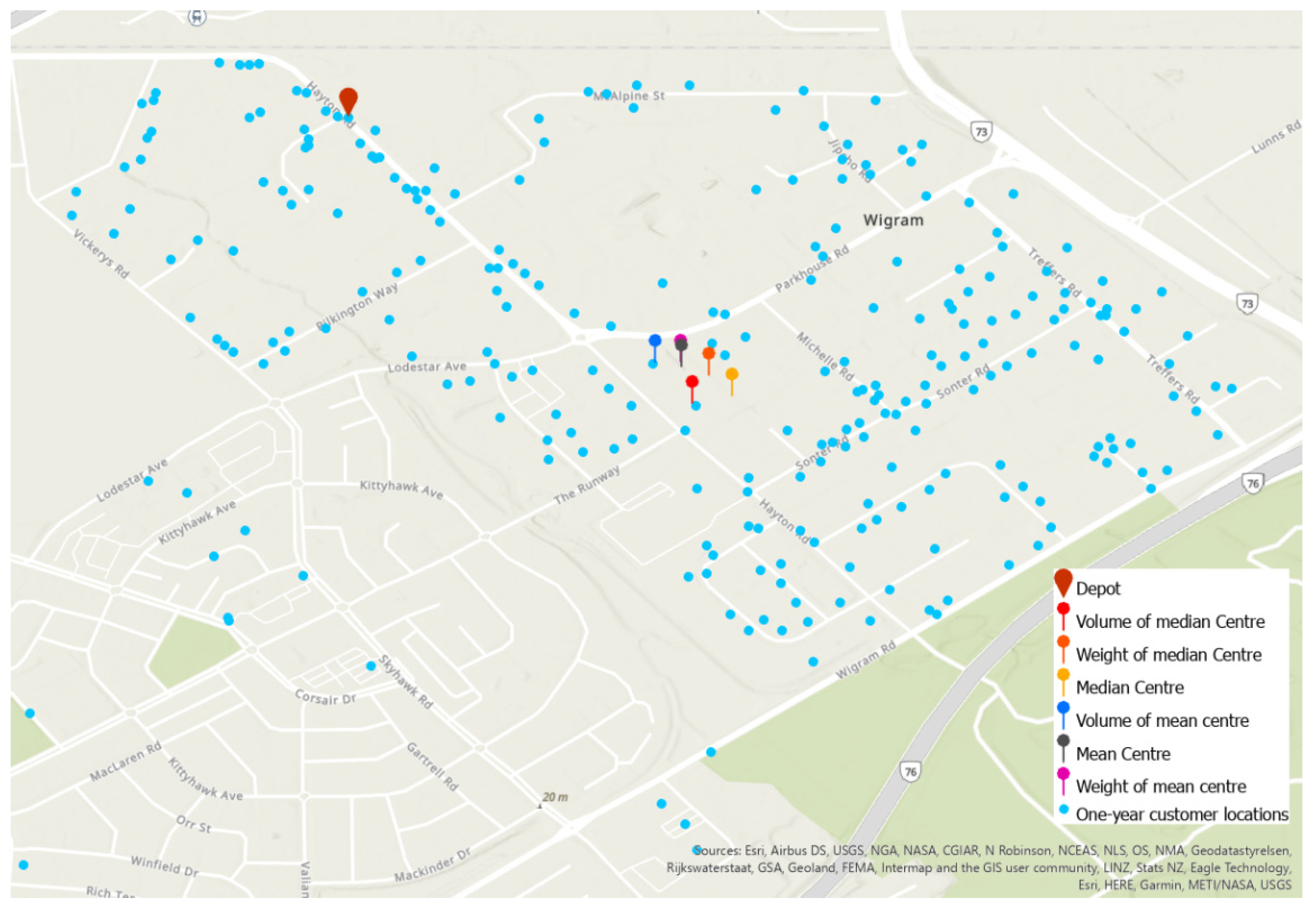
Mean centres, median centres with volume and weight attributes were calculated in ArcGIS, as shown in Figure 5. It is observed that the multiple measures of centredness are all very similar.
The mean centre identifies the geographic centre (or the centre of concentration) for a set of features. It is the average of x and y coordinates of all locations. The median centre identifies the location that minimizes the overall Euclidean distance to the location in a dataset. The mean centre is calculated by averaging x and y coordinates of all points. The mean centre ( X ¯ ,   Y ¯ )   is given as Equation (5) shows:
X ¯ = i = 1 n x i n , Y ¯ = i = 1 n y i n
where x i ,   y i are the coordinates for feature i ,   n is the total number of features. In comparison, the median centre ( x t ,   y t ) is typically found by minimising the Euclidean distance d t from each point to the centre, as Equation (6) shows. Kuhn and Kuenne [72] introduced the method of calculating the median centre, and Burt and Barber [73] provided an iterative process.
min i n d i t = ( x i x t ) 2 + ( y i y t ) 2
It is observed that the six centres are geographically similar because weight values make small differences in hotspots, as Figure 3 shows.
The purpose of the median centre is to find a centre that approximates each data point. The minimum distance was not involved in this research, so median centres were excluded. In addition, as Figure 5 shows, distributions of data points with weight, volume and consignment number are similar, which results in the mean centres with these factors being approximately coincident. From the consideration of data processing convenience, the mean centre with consignment number was selected to represent the cluster centre in the two-tier architecture, consistent with [74].
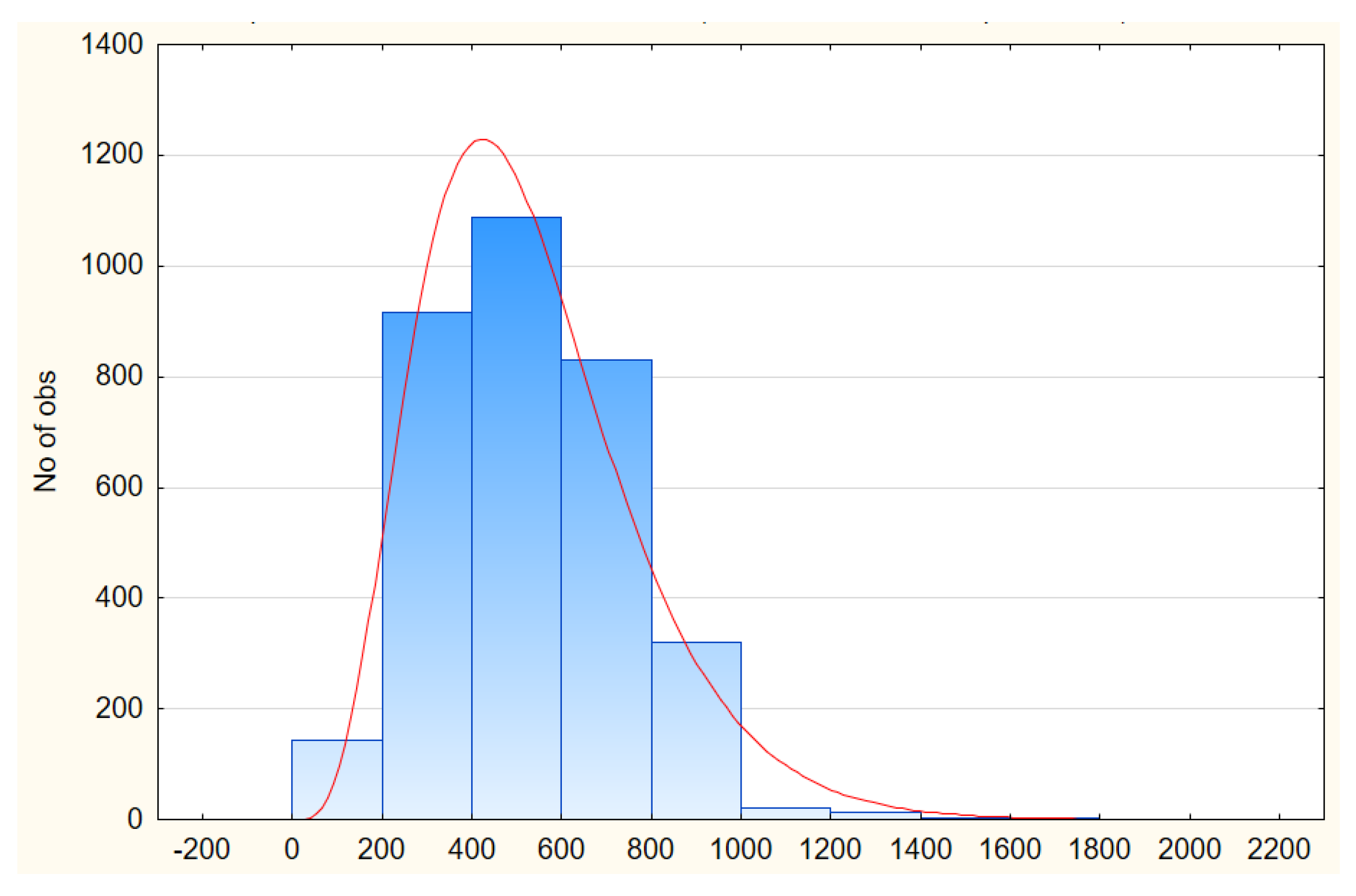
The first-tier distance ( D f ) is 762.5 m, and all Euclidean distances ( D e ) were fitted in a Gamma distribution, as shown in Figure 6. The result was computed statistically with Statistica.
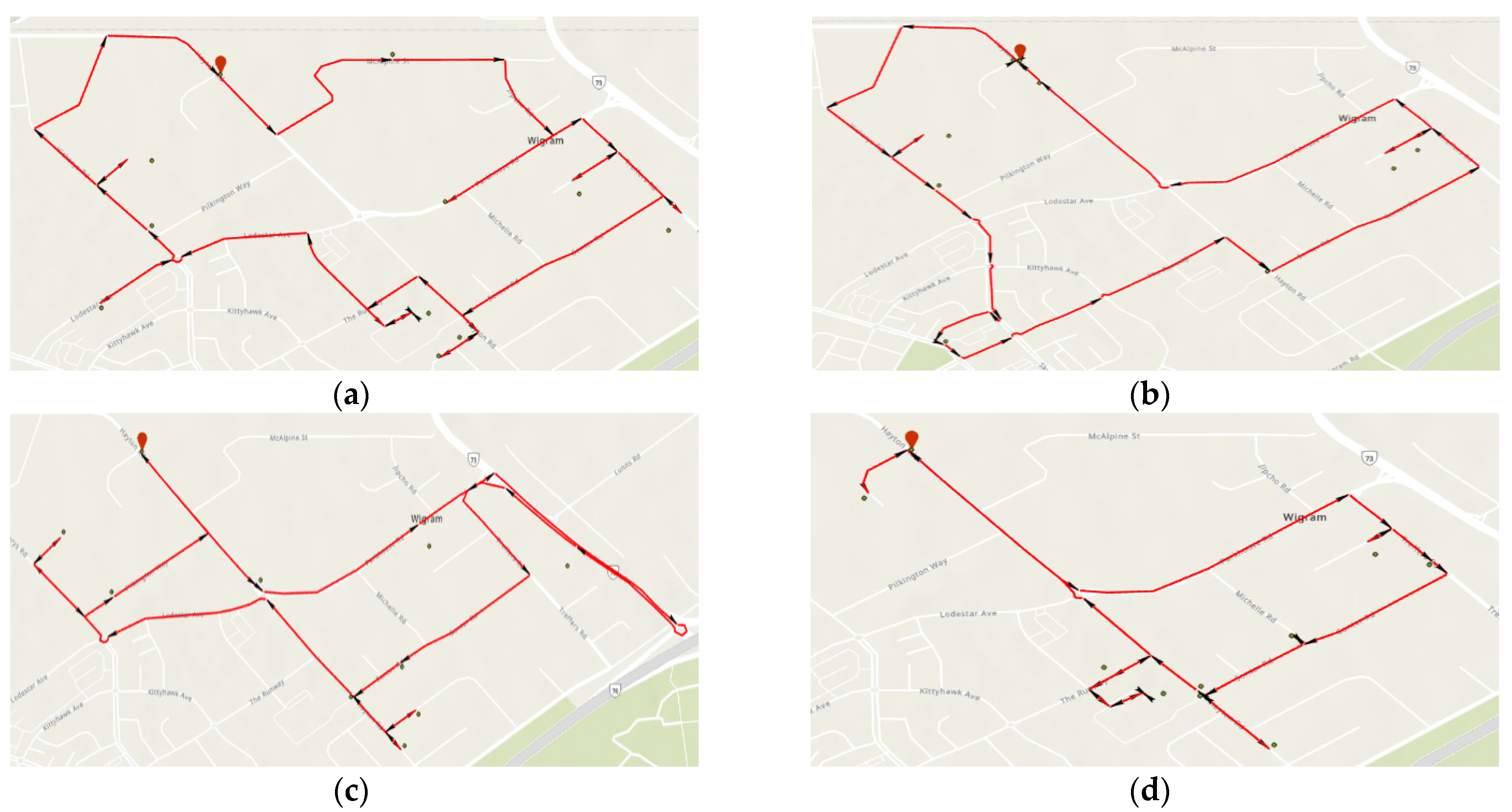
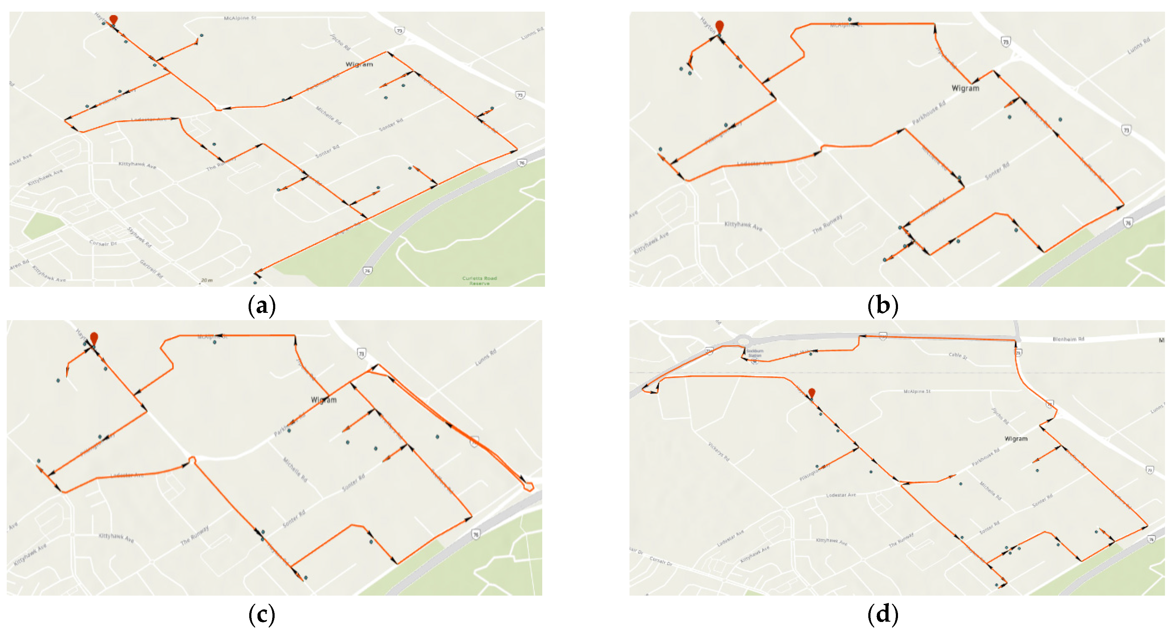
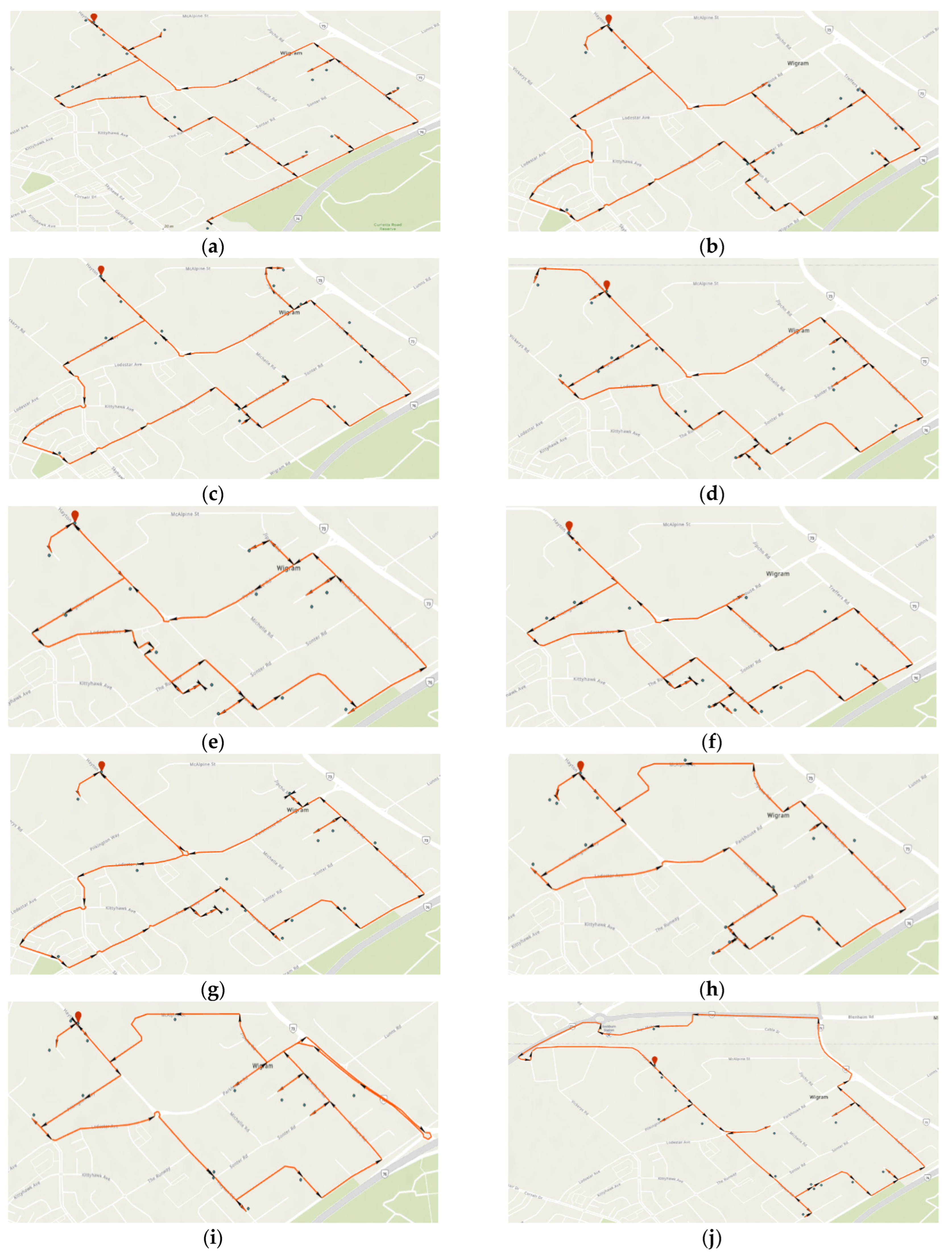
Ensembles of 10 and 15 consignment addresses were randomly selected from the consignment data. For example results of the TSP route determination for 10 and 15 consignment delivery, see Figure 7 and Figure 8, respectively. The entire results are listed in Figure A1 and Figure A2.
Note that the random selection was done by consignments, not addresses, to reflect actual operations. The difference is small, and causes the occasional duplicate address due to the consolidation process whereby one address may receive multiple consignments from different senders. The models allow the truck to economise in these cases, which is realistic. The effect is to broaden the uncertainty in the models, which is conservative.
The total distances were obtained from the two-tier architecture and TSP models. Table 4 presents the results of 10 and 15 consignment cases.
The R-value for each run was used to form a normal distribution with a mean 0.806 and a standard deviation 0.153. It was applied to n = 10, 11, 12, 13, 14, 15 cases (number of consignments). Therefore, the second-tier distance was formed through multiplying the gamma distribution and the normal distribution. Table 5 indicates the parameters of the two-tier architecture for the cluster delivery.

4.3. Results and Validation of Two-Tier Architecture

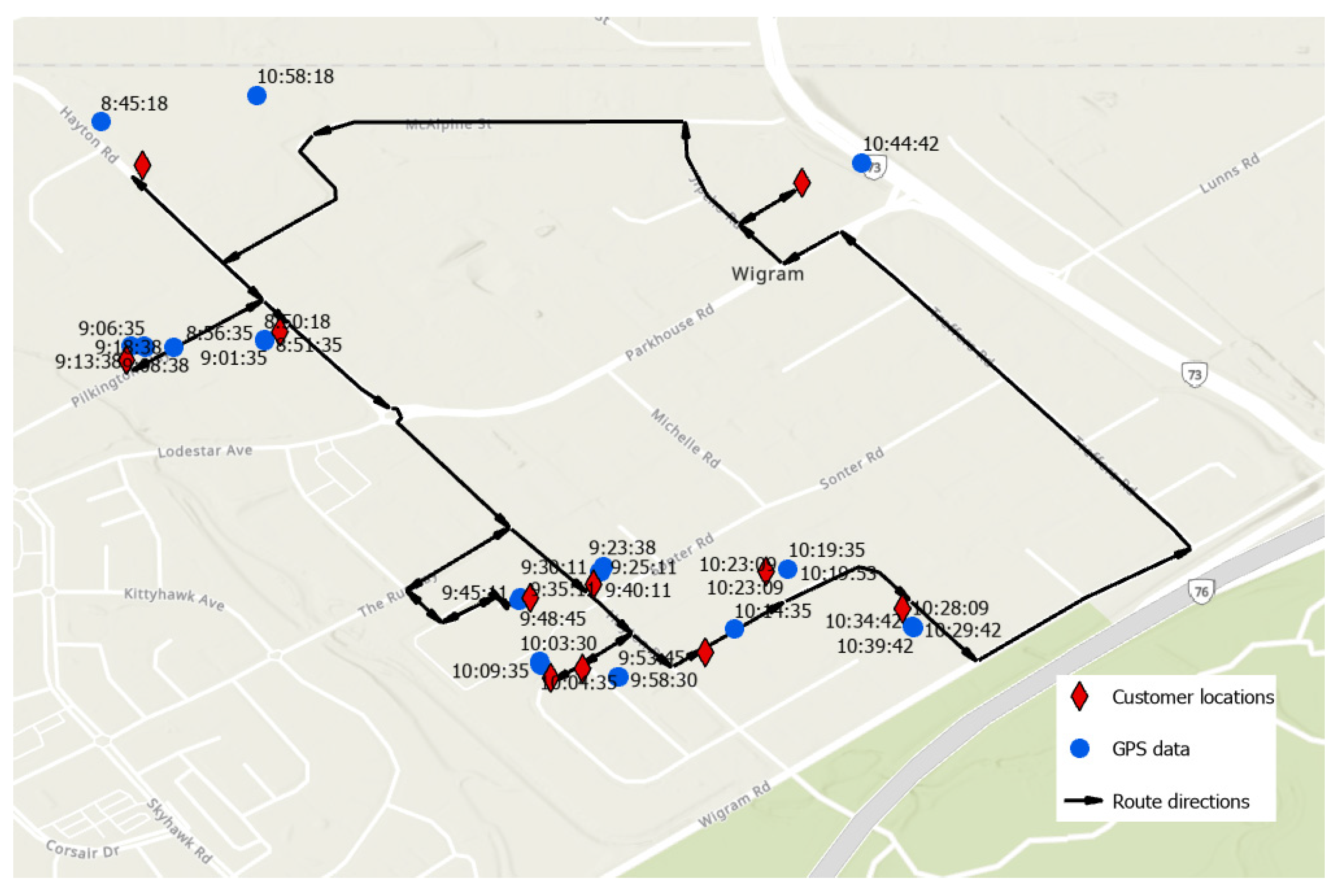
To validate the TSP simulation results, a delivery case for n = 10 was selected and the corresponding customer locations were input to ArcGIS. The TSP simulation was conducted and compared with real truck GPS data, see Figure 9.
The close correspondence between GPS and TPS results indicated that the truck driver did actually and intuitively find the optimal route to conduct the delivery. This means the TSP result can generally reflect the actually delivery route.
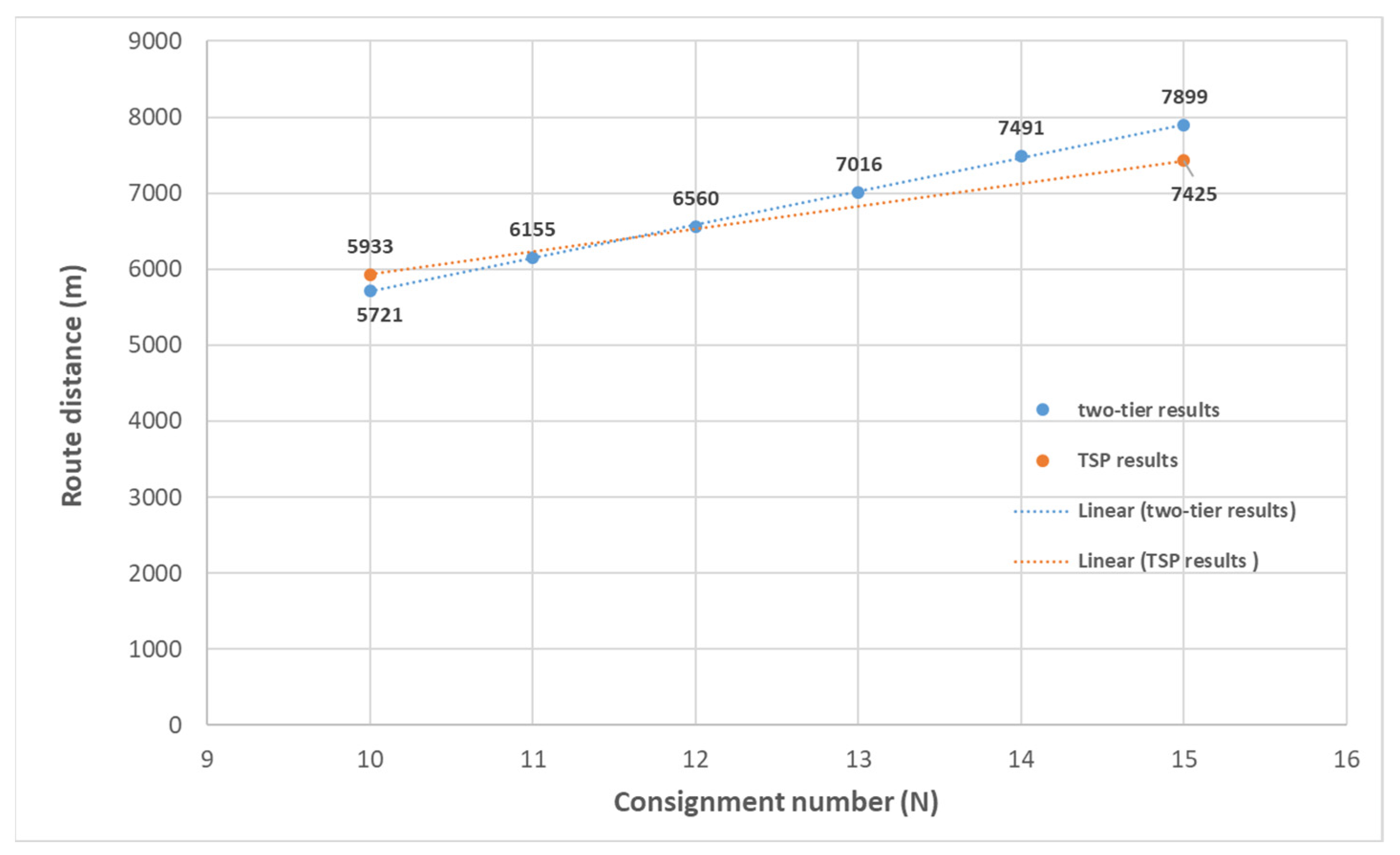
Stochastics simulations were conducted for each N case with 100 replications. All mean values of route distance are shown in Figure 10.
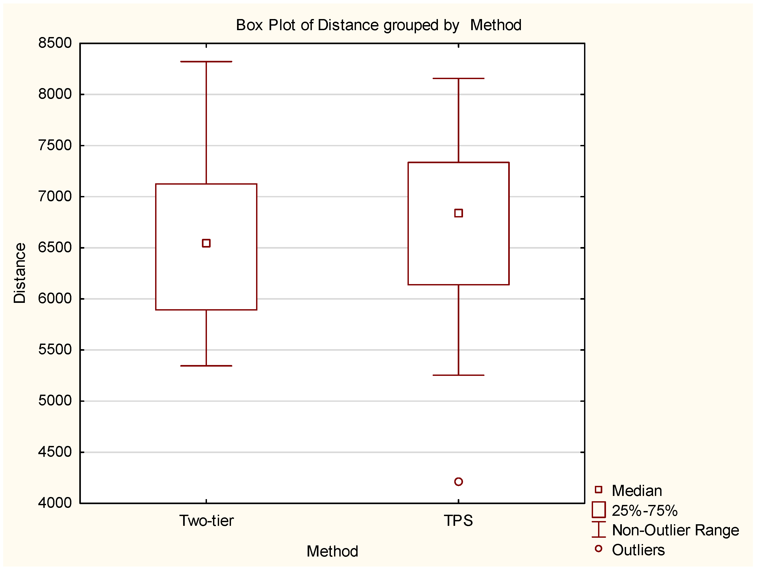
The results in Figure 10 show a reasonably close approximation for the two methods. The TSP method is the more accurate, but is not a practical method from an operational perspective because of the large amount of effort required to implement it. Hence the two-tier method has significant practical advantages. As the second stage of validation of the model, an additional set of ten TSP simulations were conducted for n = 12 using the method described above. These results were then compared to the corresponding two-tier result for n = 12. An ANOVA analysis shows the differences are not significant [F(1, 108) = 0.01745, p = 0.895], see box and whisker in Figure 11. The mean for two-tier architetcture is 6560m and for TPS 6595 m.
The validation shows distances estimated by the two-tier architecture for two cases, and the mean value is approximate to the GPS data. Therefore, freight delivery with stochastic customer locations can be validly represented by the two-tier architecture.
Hence the entire delivery last-mile region can be simplified into a cluster model with a functional dependency on the number of consignments. This potentially moves the field forward, because it allows the complexity of a variable last-mile PUD situation to be reduced into a stochastic formulation. This can be used for operational planning purposes, in real-time, by use of a suitable stochastic engine. Such an engine might be @Risk, or DES software for a more comprehensive model. A DES model could, in principle, be expanded to include multiple such suburbs, as well as the additional complexity of consolidation and line haul.
While the resulting model is relatively simple, the key enabling method is GIS. This is because the TSP algorithm within GPS provides the virtual data representing the real route. The real route could alternatively be obtained from GPS, which would be superior. However, GPS data are limited and difficult to interpret, and not always available. Furthermore, the proposed scheme using GIS overcomes the problem when the delivery runs are not yet established, as occurs in a new PUD territory.

4.4. Discrete-Event Simulation (DES) in Arena®

DES gives the opportunity to incorporate not only the distance, but also other operational realities such as time taken, truck utilisation, etc.
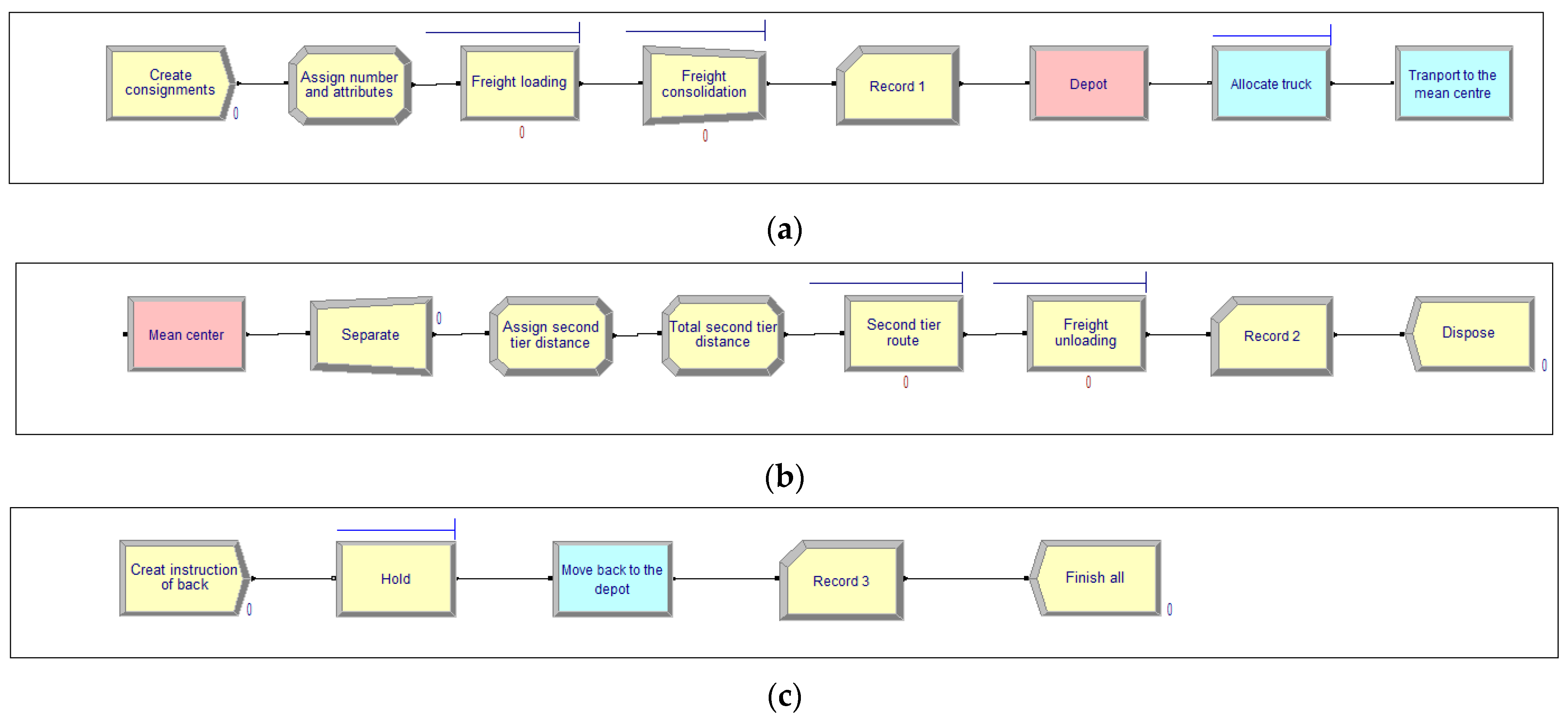
The simulation model was developed in Arena in accordance with the two-tier architecture: (a) first-tier movement, (b) second-tier movement, (c) and the return to the depot. The architecture of the DES model is shown in Figure 12.
A description of the modelling approach follows. Firstly, in Figure 12a, consignments were generated with random addresses. Then, weight and volume were assigned to each consignment from probability distributions. Freight consignments were loaded by a forklift and consolidated on the truck. The forklift was assumed to carry one consignment for each movement. Secondly, in Figure 12b, when the truck finished the first-tier movement, the truckload sequentially completed the second-tier movement with stochastic distances. The freight was assumed to be unloaded by customers. Last, after completing the transportation of all consignments, a return module was applied to the truck. As Figure 12c shows, the truck was moved back to the depot.
Simulation inputs are shown in Table 6. The truck speed and freight unloading time were obtained from the GPS data. The speed includes the truck stop and start time on roads. Distributions of consignment weight and volume were fitted based on the consignment data. The freight loading time was recorded on-site. First-tier and second-tier distances were obtained from Section 4.2.
The total time for the truck delivery Ttotal in the simulation is theoretically calculated by Equation (7).
T t o t a l = T l ( i ) + T u ( i ) + D f + D S ( i ) S   i   N

4.5. Simulation Results

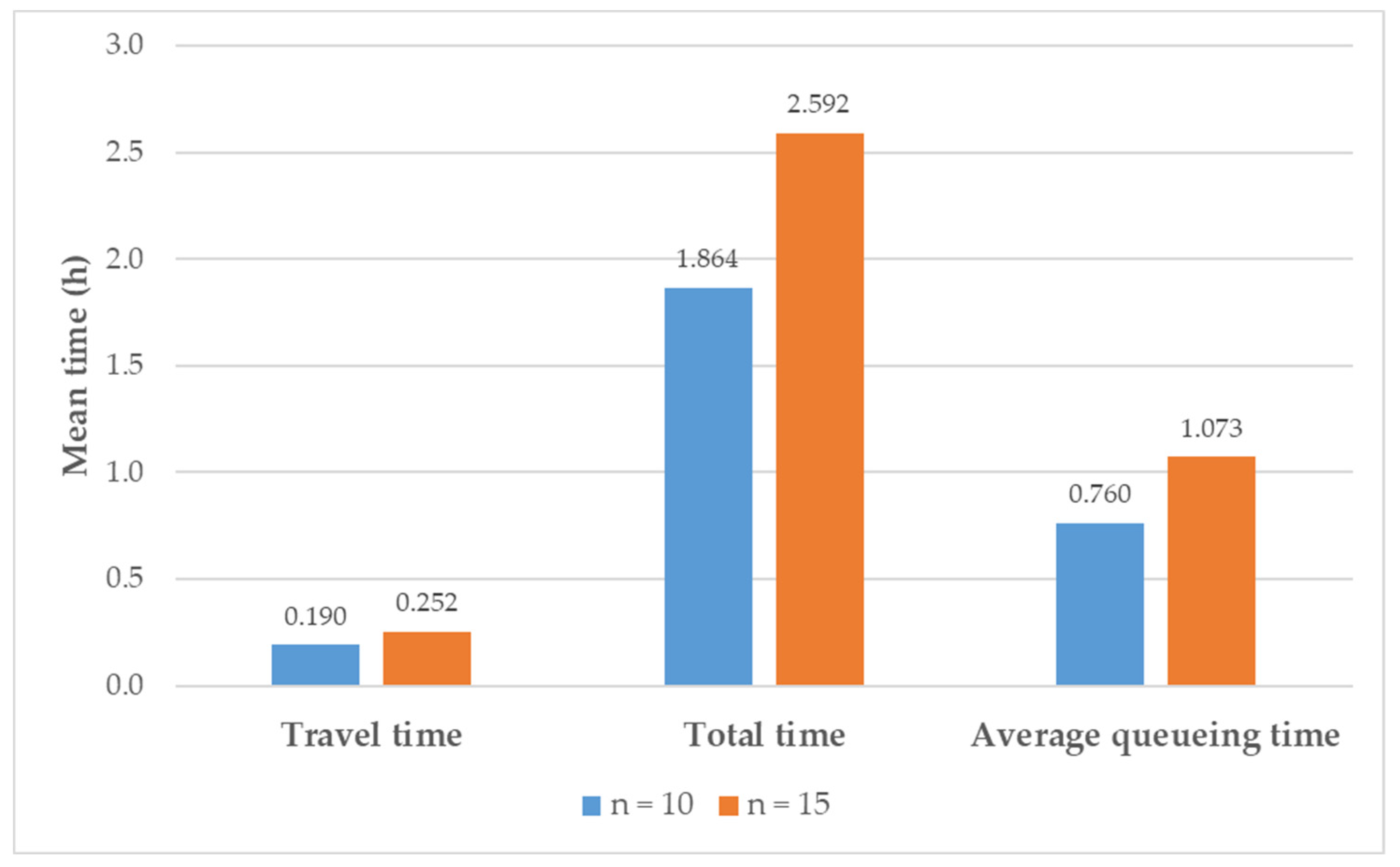
The simulation was run by 100 replications for 10 and 15 consignment cases, respectively. Figure 13 presents simulation results for time values.
The travel time accounts for a small portion of the total time in two cases. This means most of the time was spent on freight loading and unloading. In addition, the average queueing time for each consignment is large in the delivery operations. The loading and unloading activities could be improved by adding more forklifts or optimising depot operations.
The freight volume is also of concern to freight companies. The truckload weight and volume were obtained from the simulation, see Table 7. The ideal weight limit and volume limit for the PUD truck are 11 tons and 40 m3. However, the actual volume limit is 70% of the ideal limit from the consideration of health and safety, which is 28 m3.
All truckload results, including maximum values are under the truck limits. When the consignment number is 10, the capacity utilisation is low.
5. Discussion

The two-tier architecture is a possible way to describe the last-mile delivery route and can be incorporated into operational models with stochasticity. The accuracy of the architecture is high, as shown by the validation. Possible practical implications of this are predicting travel distance for an unfamiliar territory where the truck route is unknown. Travel distance is a useful proxy for the delivery time, hence order fulfilment from a customer perspective.
The operational results can be used to evaluate the freight system under different consignment volumes. In practice, this could be used as follows:
Operators, specifically drivers and dispatchers, could estimate the travel distance and the travel time for the delivery tour. The truck dispatcher can assess the capability of the current system from the results of truckload weight, truckload volume and queuing time. It is also important from an operational perspective, because the dock at the depot typically needs to be cleared each day. Stochastic truck speeds and delay times could be included to reflect unexpected traffic conditions. However, these were not incorporated into this work since the intention was to investigate distances.
Another scenario where a simple calculator like this could be useful is when the dispatchers need to determine how to split a load among multiple trucks. In this work, only the consignment number limit was considered. However, a freight consolidation module with weight and volume limits could be added to further constrain the truck capacity. Then the model could include multiple trucks. Hence the trade-off between distance and relative parameters such as fuel consumption and emissions versus speediness of customer fulfilment can be explored. There are also implications for predicting truck repair and maintenance.
A city delivery network could be constructed by several two-tier architectures of clusters. All parameters need to change because the cluster centre and TSP results are varied for clusters. As a result, this is possible to analyse the above assumptions for the whole city’s last-mile delivery.
GIS can support the construction of operational models. For specific cases, TSP can predict the truck route and distance with merely customer locations. The accuracy of this simulation is high from the comparison with real truck GPS data.

6. Conclusions

The originality of this work lies in the development of a complete workflow for highly variable PUD, incorporating a two-tier architecture informed by GIS & TSP, which is included in a DES operational model with stochasticity. The method could be used to either evaluate current freight operations or the operations for a new area. GIS was used to support the model development. TSP simulations were implemented in ArcGIS to obtain the factor R, and the accuracy was validated with real truck GPS data. A freight operations model was created and incorporated the two-tier architecture. Stochastic simulations were implemented for operational results were presented.
There are some limitations in this research. First, this research ignores pickups in the delivery run, which do occasionally occur in practice. In principle, it would not be impossible to include pickups in the DES model, see also [13]. Second, it is recommended that any practitioners who want to apply this model could expand the size of the analysis. Last, the two-tier architecture is suitable for concentrated customers rather than sparse or scattered customers. However, sparse or scattered customers can be simulated by an intersection-based model, which is also presented by [13].

Author Contributions

Conceptualization, Z.L. and D.P.; methodology, Z.L. and D.P.; software: TSP modelling, Z.L. and J.C.; DES modelling, Z.L. and J.C.; validation, Z.L. and D.P.; formal analysis, Z.L.; investigation, Z.L.; resources, Z.L. and D.P.; data curation, Z.L.; writing—original draft preparation, Z.L., J.C. and D.P.; writing—review and editing, Z.L., D.P. and Y.Z.; visualization, Z.L. and D.P.; supervision, D.P. and Y.Z.; project administration, Z.L. and D.P.; funding acquisition, Z.L. and D.P. All authors have read and agreed to the published version of the manuscript.

Funding

This research was funded by Callaghan Innovation New Zealand, grant number MAIN1901/PROP-69059-FELLOW-MAIN.

Data Availability Statement

Not applicable.

Acknowledgments

We wish to thank Mainfreight Ltd. in particular Shaun Morrow for generous assistance and support, and Ministry of Transport New Zealand for providing scholarship.

Conflicts of Interest

The authors declare no conflict of interest.

Appendix A

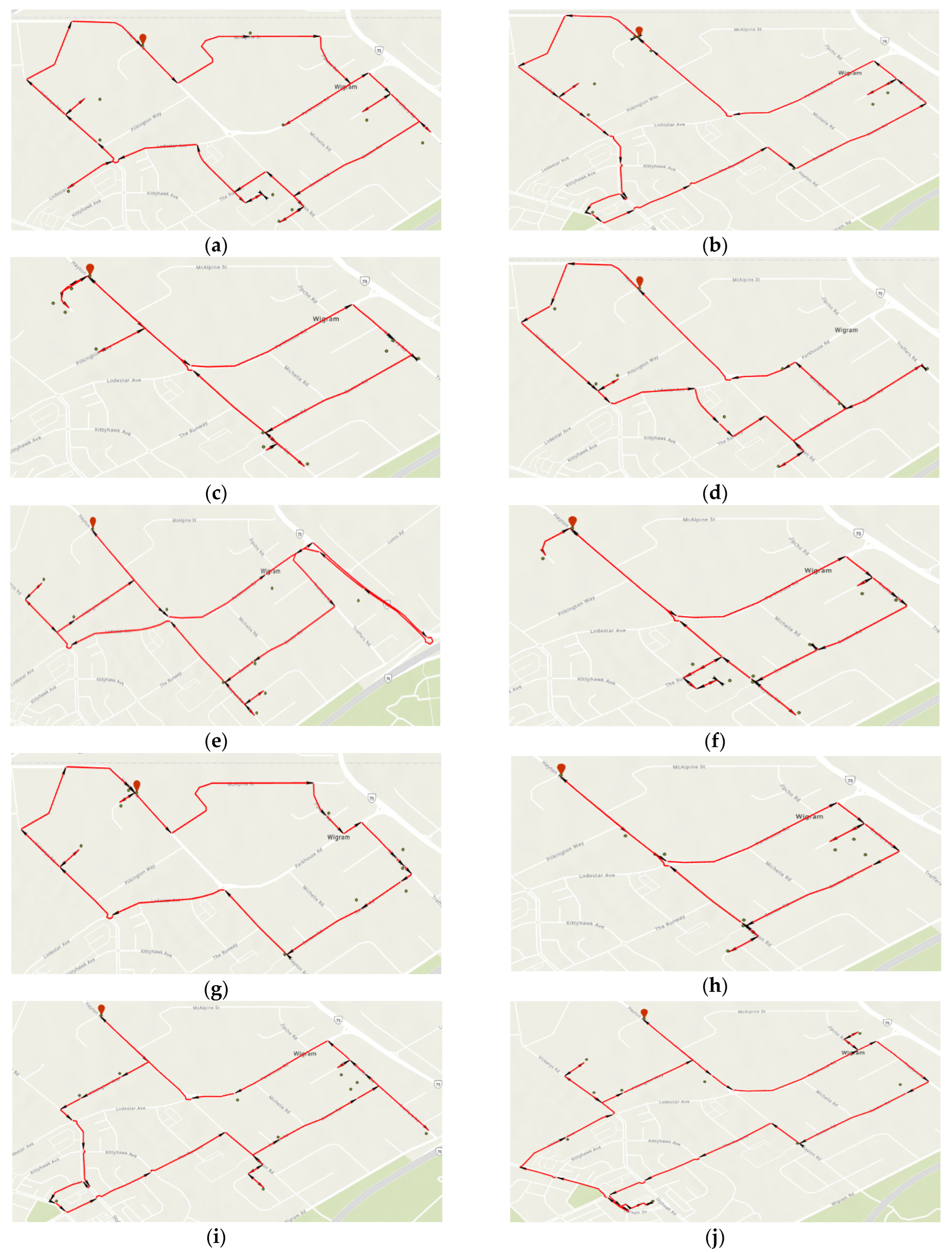
Figure A1. TSP results for 10 consignments. (a) Route one; (b) Route two; (c) Route three; (d) Route four; (e) Route five; (f) Route six; (g) Route seven; (h) Route eight; (i) Route nine; (j) Route ten.
Systems 10 00214 g0a1
Figure A2. TSP results for 15 consignments. (a) Route one; (b) Route two; (c) Route three; (d) Route four; (e) Route five; (f) Route six; (g) Route seven; (h) Route eight; (i) Route nine; (j) Route ten.
Systems 10 00214 g0a2

References

  1. Ghiani, G.; Laporte, G.; Musmanno, R. Introduction to Logistics Systems Planning and Control; J. Wiley: Hoboken, NJ, USA, 2004. [Google Scholar]
  2. Taylor, G.D. Logistics Engineering Handbook; CRC Press: Boca Raton, FL, USA, 2007. [Google Scholar] [CrossRef]
  3. Asuncion, J.; Rendall, S.; Murray, R.; Krumdieck, S. New Zealand intermodal freight network and the potential for mode shifting. In Proceedings of the New Zealand: IPENZ Transportation Group Conference, Rotorua, New Zealand, 18–21 March 2012; Available online: https://ir.canterbury.ac.nz/bitstream/handle/10092/8825/12642890_Asuncion_IPENZposter_Mar2012.pdf?sequence=1&isAllowed=y (accessed on 15 July 2022).
  4. Zakery, A. Logistics Future Trends. Logist. Oper. Manag. 2011, 6, 93–105. [Google Scholar] [CrossRef]
  5. Hlupic, V.; Robinson, S. Successful Simulation: A Practical Approach to Simulation Projects. J. Oper. Res. Soc. 1995, 46, 915. [Google Scholar] [CrossRef]
  6. Amorim-Lopes, M.; Guimarães, L.; Alves, J.; Almada-Lobo, B. Improving picking performance at a large retailer warehouse by combining probabilistic simulation, optimization, and discrete-event simulation. Int. Trans. Oper. Res. 2020, 28, 687–715. [Google Scholar] [CrossRef]
  7. Marinov, M.; Viegas, J. A mesoscopic simulation modelling methodology for analyzing and evaluating freight train operations in a rail network. Simul. Model. Pr. Theory 2011, 19, 516–539. [Google Scholar] [CrossRef]
  8. Mommens, K.; Lebeau, P.; Verlinde, S.; van Lier, T.; Macharis, C. Evaluating the impact of off-hour deliveries: An application of the TRansport Agent-BAsed model. Transp. Res. Part D: Transp. Environ. 2018, 62, 102–111. [Google Scholar] [CrossRef]
  9. Lu, S.; Xin, B.; Zhang, H.; Chen, J. Agent-based Self-organized Constructive Heuristics for Travelling Salesman Problem. In Proceedings of the 2020 59th IEEE Conference on Decision and Control (CDC), Jeju, Korea, 14–18 December 2020; pp. 1164–1169. [Google Scholar] [CrossRef]
  10. Dantzig, G.B.; Ramser, J.H. The Truck Dispatching Problem. Manag. Sci. 1959, 6, 80–91. [Google Scholar] [CrossRef]
  11. Hopkins, D.; McCarthy, A. Change trends in urban freight delivery: A qualitative inquiry. Geoforum 2016, 74, 158–170. [Google Scholar] [CrossRef] [Green Version]
  12. Lyu, Z.; Pons, D.; Zhang, Y.; Ji, Z. Minimum Viable Model (MVM) Methodology for Integration of Agile Methods into Operational Simulation of Logistics. Logistics 2022, 6, 37. [Google Scholar] [CrossRef]
  13. Lyu, Z.; Pons, D.; Zhang, Y.; Ji, Z. Freight Operations Modelling for Urban Delivery and Pickup with Flexible Routing: Cluster Transport Modelling Incorporating Discrete-Event Simulation and GIS. Infrastructures 2021, 6, 180. [Google Scholar] [CrossRef]
  14. Aliahmadi, S.Z.; Barzinpour, F.; Pishvaee, M.S. A fuzzy optimization approach to the capacitated node-routing problem for municipal solid waste collection with multiple tours: A case study. Waste Manag. Res. J. a Sustain. Circ. Econ. 2019, 38, 279–290. [Google Scholar] [CrossRef]
  15. Salazar-Aguilar, M.A.; Langevin, A.; Laporte, G. The synchronized arc and node routing problem: Application to road marking. Comput. Oper. Res. 2013, 40, 1708–1715. [Google Scholar] [CrossRef]
  16. Kumar, A. Improved Genetic Algorithm to Solve Small Scale Travelling Salesman Problem. In Proceedings of the 2020 4th International Conference on Intelligent Computing and Control Systems, Madurai, India, 13–15 May 2020; pp. 516–520. [Google Scholar] [CrossRef]
  17. Agrawal, M.; Jain, V. Applying Improved Genetic Algorithm to Solve Travelling Salesman Problem. In Proceedings of the 2020 Second International Conference on Inventive Research in Computing Applications, Coimbatore, India, 15–17 July 2020; pp. 1194–1197. [Google Scholar] [CrossRef]
  18. Silva, B.C.; Fernandes, I.F.d.C.; Goldbarg, M.C.; Goldbarg, E.F. Quota travelling salesman problem with passengers, incomplete ride and collection time optimization by ant-based algorithms. Comput. Oper. Res. 2020, 120, 104950. [Google Scholar] [CrossRef]
  19. Zbib, H.; Laporte, G. The commodity-split multi-compartment capacitated arc routing problem. Comput. Oper. Res. 2020, 122, 104994. [Google Scholar] [CrossRef]
  20. Amini, A.; Tavakkoli-Moghaddam, R.; Ebrahimnejad, S. A bi-objective transportation-location arc routing problem. Transp. Lett. 2019, 12, 623–637. [Google Scholar] [CrossRef]
  21. Padungwech, W.; Thompson, J.; Lewis, R. Effects of update frequencies in a dynamic capacitated arc routing problem. Networks 2020, 76, 522–538. [Google Scholar] [CrossRef]
  22. Campbell, J.F.; Corberán, Á.; Plana, I.; Sanchis, J.M.; Segura, P. Solving the length constrained K-drones rural postman problem. Eur. J. Oper. Res. 2020, 292, 60–72. [Google Scholar] [CrossRef]
  23. Benavent, E.; Corberán, Á.; Laganà, D.; Vocaturo, F. The periodic rural postman problem with irregular services on mixed graphs. Eur. J. Oper. Res. 2019, 276, 826–839. [Google Scholar] [CrossRef]
  24. Afanasev, V.A.; van Bevern, R.; Tsidulko, O.Y. The Hierarchical Chinese Postman Problem: The slightest disorder makes it hard, yet disconnectedness is manageable. Oper. Res. Lett. 2021, 49, 270–277. [Google Scholar] [CrossRef]
  25. Siloi, I.; Carnevali, V.; Pokharel, B.; Fornari, M.; Di Felice, R. Investigating the Chinese postman problem on a quantum annealer. Quantum Mach. Intell. 2021, 3, 1–10. [Google Scholar] [CrossRef]
  26. Majumder, S.; Kar, S.; Pal, T. Uncertain multi-objective Chinese postman problem. Soft Comput. 2018, 23, 11557–11572. [Google Scholar] [CrossRef]
  27. Llorca, C.; Moeckel, R. Assesment of the potential of cargo bikes and electrification for last-mile parcel delivery by means of simulation of urban freight flows. Eur. Transp. Res. Rev. 2021, 13, 1–14. [Google Scholar] [CrossRef]
  28. Melkonyan, A.; Gruchmann, T.; Lohmar, F.; Kamath, V.; Spinler, S. Sustainability assessment of last-mile logistics and distribution strategies: The case of local food networks. Int. J. Prod. Econ. 2020, 228, 107746. [Google Scholar] [CrossRef]
  29. Wang, C.-N.; Nguyen, N.-A.; Dang, T.-T.; Hsu, H.-P. Evaluating Sustainable Last-Mile Delivery (LMD) in B2C E-Commerce Using Two-Stage Fuzzy MCDM Approach: A Case Study From Vietnam. IEEE Access 2021, 9, 146050–146067. [Google Scholar] [CrossRef]
  30. Aized, T.; Srai, J.S. Hierarchical modelling of Last Mile logistic distribution system. Int. J. Adv. Manuf. Technol. 2013, 70, 1053–1061. [Google Scholar] [CrossRef]
  31. Ghaderi, H.; Tsai, P.-W.; Zhang, L.; Moayedikia, A. An integrated crowdshipping framework for green last mile delivery. Sustain. Cities Soc. 2021, 78, 103552. [Google Scholar] [CrossRef]
  32. Jiang, L.; Zang, X.; Alghoul, I.I.; Fang, X.; Dong, J.; Liang, C. Scheduling the covering delivery problem in last mile delivery. Expert Syst. Appl. 2021, 187, 115894. [Google Scholar] [CrossRef]
  33. Franceschetti, A.; Jabali, O.; Laporte, G. Continuous approximation models in freight distribution management. TOP 2017, 25, 413–433. [Google Scholar] [CrossRef]
  34. Simoni, M.D.; Marcucci, E.; Gatta, V.; Claudel, C.G. Potential last-mile impacts of crowdshipping services: A simulation-based evaluation. Transportation 2020, 47, 1933–1954. [Google Scholar] [CrossRef]
  35. Oyola, J.; Arntzen, H.; Woodruff, D.L. The stochastic vehicle routing problem, a literature review, part I: Models. EURO J. Transp. Logist. 2016, 7, 193–221. [Google Scholar] [CrossRef]
  36. Oyola, J.; Arntzen, H.; Woodruff, D.L. The stochastic vehicle routing problem, a literature review, Part II: Solution methods. EURO J. Transp. Logist. 2016, 6, 349–388. [Google Scholar] [CrossRef]
  37. Altiok, T.; Melamed, B. Simulation Modeling and Analysis with ARENA; Academic Press: Cambridge, MA, USA, 2007; Volume 1, pp. 1–10. [Google Scholar] [CrossRef]
  38. Jahangirian, M.; Eldabi, T.; Naseer, A.; Stergioulas, L.K.; Young, T. Simulation in manufacturing and business: A review. Eur. J. Oper. Res. 2010, 203, 1–13. [Google Scholar] [CrossRef] [Green Version]
  39. Motraghi, A.; Marinov, M.V. Analysis of urban freight by rail using event based simulation. Simul. Model. Pract. Theory 2012, 25, 73–89. [Google Scholar] [CrossRef]
  40. Zhao, Y.; Ioannou, P.A.; Dessouky, M.M. Dynamic Multimodal Freight Routing Using a Co-Simulation Optimization Approach. IEEE Trans. Intell. Transp. Syst. 2018, 20, 2657–2667. [Google Scholar] [CrossRef]
  41. Rezaeifar, F.; Najafi, M.; Kaushal, V.; Huff, B. Development of a Model to Optimize the Operations of an Intermodal Underground Logistics Transportation. J. Pipeline Syst. Eng. Pr. 2022, 13, 04022039. [Google Scholar] [CrossRef]
  42. Li, L.; Qiu, M.; Wu, B.; Wang, X. Simulation Research on Road Transport in Container Port Based on Arena. ICLEM 2010 2010, 1, 1880–1888. [Google Scholar] [CrossRef]
  43. Reggelin, T.; Lang, S.; Schauf, C. Mesoscopic discrete-rate-based simulation models for production and logistics planning. J. Simul. 2020, 16, 448–457. [Google Scholar] [CrossRef]
  44. Hashemi, A.S.; Sattarvand, J. Application of ARENA Simulation Software for Evaluation of Open Pit Mining Transportation Systems—A Case Study; Springer: Cham, Switzerland, 2015; pp. 213–224. [Google Scholar] [CrossRef]
  45. Jaoua, A.; Riopel, D.; Gamache, M. A simulation framework for real-time fleet management in internal transport systems. Simul. Model. Pr. Theory 2012, 21, 78–90. [Google Scholar] [CrossRef]
  46. Reiffer, A.; Kübler, J.; Briem, L.; Kagerbauer, M.; Vortisch, P. Integrating Urban Last-Mile Package Deliveries into an Agent-Based Travel Demand Model. Procedia Comput. Sci. 2021, 184, 178–185. [Google Scholar] [CrossRef]
  47. Govindan, K.; Fattahi, M.; Keyvanshokooh, E. Supply chain network design under uncertainty: A comprehensive review and future research directions. Eur. J. Oper. Res. 2017, 263, 108–141. [Google Scholar] [CrossRef]
  48. Boile, M.P. Intermodal transportation network analysis-a GIS application. In Proceedings of the 2000 10th Mediterranean Electrotechnical Conference. Information Technology and Electrotechnology for the Mediterranean Countries, Lemesos, Cyprus, 29–31 May 2000. [Google Scholar]
  49. Winebrake, J.J.; Corbett, J.J.; Falzarano, A.; Hawker, J.S.; Korfmacher, K.; Ketha, S.; Zilora, S. Assessing Energy, Environmental, and Economic Tradeoffs in Intermodal Freight Transportation. J. Air Waste Manag. Assoc. 2008, 58, 1004–1013. [Google Scholar] [CrossRef] [Green Version]
  50. Akay, A.E.; Wing, M.G.; Sivrikaya, F.; Sakar, D. A GIS-based decision support system for determining the shortest and safest route to forest fires: A case study in Mediterranean Region of Turkey. Environ. Monit. Assess. 2012, 184, 1391–1407. [Google Scholar] [CrossRef] [PubMed]
  51. Wang, K. Application of Cloud Computing and GIS Based on Internet of Things in Oil and Gas Storage and Transportation Production Management and Safety Monitoring and Early Warning System. Mob. Inf. Syst. 2022, 2022, 1–11. [Google Scholar] [CrossRef]
  52. Jiao, J.; Liu, Y.; Xie, C. The Optimization Model of E-Commerce Logistics Distribution Path Based on GIS Technology. Adv. Multimedia 2022, 2022, 1–9. [Google Scholar] [CrossRef]
  53. Vu, H.L.; Ng, K.T.W.; Fallah, B.; Richter, A.; Kabir, G. Interactions of residential waste composition and collection truck compartment design on GIS route optimization. Waste Manag. 2019, 102, 613–623. [Google Scholar] [CrossRef]
  54. Hemidat, S.; Oelgemöller, D.; Nassour, A.; Nelles, M. Evaluation of Key Indicators of Waste Collection Using GIS Techniques as a Planning and Control Tool for Route Optimization. Waste Biomass- Valorization 2017, 8, 1533–1554. [Google Scholar] [CrossRef]
  55. Jwad, Z.A.; Hasson, S.T. An Optimization Approach for Waste Collection Routes Based on GIS in Hillah-Iraq. In Proceedings of the 2018 International Conference on Advanced Science and Engineering (ICOASE), Duhok, Iraq, 9–11 October 2018; pp. 60–63. [Google Scholar] [CrossRef]
  56. Vu, H.L.; Bolingbroke, D.; Ng, K.T.W.; Fallah, B. Assessment of waste characteristics and their impact on GIS vehicle collection route optimization using ANN waste forecasts. Waste Manag. 2019, 88, 118–130. [Google Scholar] [CrossRef]
  57. Ransikarbum, K.; Mason, S.J. A bi-objective optimisation of post-disaster relief distribution and short-term network restoration using hybrid NSGA-II algorithm. Int. J. Prod. Res. 2021, 60, 1–30. [Google Scholar] [CrossRef]
  58. Tosarkani, B.M.; Amin, S.H.; Zolfagharinia, H. A scenario-based robust possibilistic model for a multi-objective electronic reverse logistics network. Int. J. Prod. Econ. 2019, 224, 107557. [Google Scholar] [CrossRef]
  59. De Bittencourt, G.C.; Chagas, R.D.S.; Silva, V.A.; Vianna, I.G.P.; Longhi, R.P.; Ribas, P.C.; Filho, V.J.M.F. A solution framework for the integrated problem of cargo assignment, fleet sizing, and delivery planning in offshore logistics. Comput. Ind. Eng. 2021, 161, 107653. [Google Scholar] [CrossRef]
  60. Juan, A.A.; Faulin, J.; Grasman, S.E.; Rabe, M.; Figueira, G. A review of simheuristics: Extending metaheuristics to deal with stochastic combinatorial optimization problems. Oper. Res. Perspect. 2015, 2, 62–72. [Google Scholar] [CrossRef] [Green Version]
  61. Hazaymeh, K.; Almagbile, A.; Alomari, A.H. Spatiotemporal Analysis of Traffic Accidents Hotspots Based on Geospatial Techniques. ISPRS Int. J. Geo-Inf. 2022, 11, 260. [Google Scholar] [CrossRef]
  62. Zhou, Y.; Yu, H.; and Cai, X. A novel k-means algorithm for clustering and outlier detection. In Proceedings of the 2009 Second International Conference on Future Information Technology and Management Engineering, Sanya, China, 13–14 December 2009. [Google Scholar]
  63. Loganathan, S.; Arumugam, J. Energy centroid clustering algorithm to enhance the network lifetime of wireless sensor networks. Multidimens. Syst. Signal Process. 2019, 31, 829–856. [Google Scholar] [CrossRef]
  64. Kwon, J.-H.; Kim, E.-J. Machine Failure Analysis Using Nearest Centroid Classification for Industrial Internet of Things. Sensors Mater. 2019, 31, 1751. [Google Scholar] [CrossRef]
  65. Thalamala, R.; Barnabas, J.; Reddy, A. A novel variant of social spider optimization using single centroid representation and enhanced mating for data clustering. PeerJ Comput. Sci. 2019, 5, e201. [Google Scholar] [CrossRef] [Green Version]
  66. Liu, R.; Yang, Z.; Chen, Q.; Liao, G.; Zhen, W. GNSS Multi-Interference Source Centroid Location Based on Clustering Centroid Convergence. IEEE Access 2021, 9, 108452–108465. [Google Scholar] [CrossRef]
  67. He, Q.; Chen, Z.; Ji, K.; Wang, L.; Ma, K.; Zhao, C.; Shi, Y. Cluster Center Initialization and Outlier Detection Based on Distance and Density for the K-Means Algorithm; Springer: Cham, Switzerland, 2019; pp. 530–539. [Google Scholar] [CrossRef]
  68. Li, S.; Liu, Z.; Zhao, H. K-means Clustering Method Based on Kernel Density Estimation to Analysis Residents Travel Features: A Case Study of Chengdu. J. Physics Conf. Ser. 2020, 1646, 12–18. [Google Scholar] [CrossRef]
  69. Anderson, T.K. Kernel density estimation and K-means clustering to profile road accident hotspots. Accid. Anal. Prev. 2009, 41, 359–364. [Google Scholar] [CrossRef]
  70. Xu, S.; Bie, R.; Li, L.; Yang, Y. DP-Dip: A skinny method for estimating the number and center of clusters. Procedia Comput. Sci. 2018, 129, 2–8. [Google Scholar] [CrossRef]
  71. Zhou, Y.; Xie, R.; Zhang, T.; Holguin-Veras, J. Joint Distribution Center Location Problem for Restaurant Industry Based on Improved K-Means Algorithm With Penalty. IEEE Access 2020, 8, 37746–37755. [Google Scholar] [CrossRef]
  72. Kulin, H.W.; Kuenne, R.E. AN EFFICIENT ALGORITHM FOR THE NUMERICAL SOLUTION OF THE GENERALIZED WEBER PROBLEM IN SPATIAL ECONOMICS. J. Reg. Sci. 1962, 4, 21–33. [Google Scholar] [CrossRef]
  73. Burt, J.; Barber, G. 1996: Elementary Statistics for Geographers; The Guilford Press: New York, NY, USA, 1996. [Google Scholar]
  74. Dhanachandra, N.; Manglem, K.; Chanu, Y.J. Image Segmentation Using K -means Clustering Algorithm and Subtractive Clustering Algorithm. Procedia Comput. Sci. 2015, 54, 764–771. [Google Scholar] [CrossRef]
Figure 1. Schematic of two-tier architecture.
Systems 10 00214 g001
Figure 2. Simulation model development process.
Systems 10 00214 g002
Figure 3. Freight delivery operations.
Systems 10 00214 g003
Figure 4. Hotspots of consignment data with attributes (a) Attribute of consignment number; (b) Attribute of consignment weight; (c) Attribute of consignment volume.
Systems 10 00214 g004
Figure 5. Customer locations and cluster centres.
Systems 10 00214 g005
Figure 6. The Euclidean distance (De) with a Gamma distribution fit with scale 107.3192 and shape 4.9074.
Systems 10 00214 g006
Figure 7. TSP results for n = 10 delivery routes. (a) Example one; (b) Example two; (c) Example three; (d) Example four.
Systems 10 00214 g007
Figure 8. TSP results for n = 15 delivery routes. (a) Example one; (b) Example two; (c) Example three; (d) Example four.
Systems 10 00214 g008
Figure 9. TSP route and GPS data for an n = 10 case.
Systems 10 00214 g009
Figure 10. Mean values of route distance for different N cases for two-tier simulation (blue) compared to TSP results (orange). TSP results are only shown for n = 10 and 15.
Systems 10 00214 g010
Figure 11. Box plot with medians and percentiles for Two-tier and TSP for n = 12 cases.
Systems 10 00214 g011
Figure 12. DES delivery model: (a) first-tier movement; (b) second-tier movement; (c) the return to the depot.
Systems 10 00214 g012
Figure 13. Mean values for times with logistics model using two-tier sub-model.
Systems 10 00214 g013
Table 1. Summary of last-mile delivery modelling methods.
MethodsDescriptionExamples of Approaches That Have Been Attempted
Mathematical models (VRP)Typical VPR models include NRP, TSP and ARP models. Mathematical models can be developed easily and rapidly. However, these models need to simplify the real system with little stochasticity. [14,15,16,17,18,19,20,21]
Computer simulation models These models can simulate complex systems with a large number of uncertainties. The disadvantages are the long modelling period and the difficulty of representing specific routes. [39,40]
GIS models GIS is able to find routes by implementing VRP algorithms, but it is limited to standalone cases.[53,54,55,56]
Integration of mathematical, simulation and GIS modelsHigh daily variability in consignment/customer addresses, and number of consignments requires that the model be recomputed each time. The integration tends to be applied manually, rather than completely automated, so this takes time. For this reason, existing integration systems may not yet be ready for routine operational use in the industry. [57,58]
Table 2. Key assumptions.
ParametersAssumptions
Number of consignments10 and 15
AddressesRandomly selected
Truck capacityOne truck is sufficient for assumed consignment numbers
Truck speedAverage speed including truck stop and start times
BackhaulNone
Table 3. The proportion of consignment data for suburbs.
AreaCount of ConsignmentsSum of WeightSum of Volume
Wigram69.26%70.16%74.74%
Sockburn26.23%25.55%21.63%
Central city1.03%2.23%1.05%
Addington0.94%0.32%0.78%
Hornby0.57%0.42%0.42%
Halswell0.54%0.30%0.47%
Upper Riccarton 0.26%0.18%0.10%
Sydenham0.11%0.05%0.06%
Harewood0.11%0.10%0.08%
Hillmorton0.09%0.06%0.09%
Middleton0.09%0.06%0.05%
Waltham0.06%0.02%0.01%
Riccarton0.06%0.21%0.22%
Templeton0.03%0.00%0.01%
Islington0.03%0.00%0.01%
Wainoni0.03%0.01%0.02%
Bishopdale0.03%0.01%0.03%
Airport0.03%0.00%0.00%
Hoon Hay0.03%0.01%0.04%
Hornby South0.03%0.07%0.02%
Unknown data0.46%0.23%0.20%
Table 4. Result of 10 and 15 consignment cases.
Number of ConsignmentsDelivery CaseTotal Second-Tier Distance D S (m)Total Distance for Two-Tier Architecture D t o t a l (m)Total Distance for TSP D t (m)R-Value
n = 1015265679076451.163
26176770160660.735
36152767749060.550
44557608254170.854
55248677374591.131
64191571651750.871
75840736552410.636
83712523741150.698
95439696463970.896
105905743069060.911
n = 1518337986179560.771
28126965172420.704
37999952474160.736
48385991073110.690
56694821971310.837
66988851364260.701
76951847675990.874
87750927565840.653
98099962486740.883
107701922679120.829
Table 5. Parameters for the two-tier architecture of the cluster.
Two-Tier Parameters
D f (m)762.5
D s (m) D e R = GAMM(107.319, 4.907) ∗ NORM(0.806, 0.153)
Table 6. Simulation input variables.
Parameter VariableValue
Consignment number N10 and 15
Truck speed (km/h)S30.893
Consignment weight (kg)W0.999 + EXPO(409)
Consignment volume (m3)V−0.001 + EXPO(1.38)
Freight loading time (s)Tl26 + EXPO(21.6)
Freight unloading time (min)Tu0.5 + GAMM(7.81, 1.15)
First-tier distance (m)Df762.5
Second-tier distance (m)DsGAMM(107.319, 4.907) ∗ NORM(0.806, 0.153)
Table 7. Freight attribute results.
n = 10n = 15
Truckload weight (t)mean4.1256.261
std dvn1.2071.511
Truckload volume (m3)mean13.50620.513
std dvn3.7695.374
Capacity utilisation mean48%73%
Publisher’s Note: MDPI stays neutral with regard to jurisdictional claims in published maps and institutional affiliations.