Early Warning of Systemic Financial Risk of Local Government Implicit Debt Based on BP Neural Network Model

Abstract

In recent years, local governments have boosted their local economies by raising large amounts of debt. Even though the state further strictly controls local government debt, the hidden debt formed by the local government borrowing in disguised form can infect systemic financial risks, creating an urgent need to carry out risk warning based on local government hidden debt. The paper uses the macro indicators of local government implicit debt risk at the prefecture-level city level, and introduces the micro indicators of PPP projects, financing platform bank debt, and urban investment debt to establish a BP neural network model. We not only study the contagion effect of local government hidden debt on systemic financial risks, but also predict the systemic financial risks in 2019 and construct an early warning risk system based on the prefecture-level city data from 2015 to 2018. In addition, the early warning effect of local government implicit debt on systemic financial risk under different stress scenarios is investigated. The study found that the implicit debt risk of local governments, the scale of financing platform bank debt, the scale of PPP, and the scale of urban investment bonds have a significant impact on systemic financial risks. The neural network model constructed by introducing these four variables at the same time can better predict the level of systemic financial risk. The model can also accurately predict the changes in systemic financial risks under the stress test of the increase in hidden debt of different local governments, and has a good early warning effect.

1. Introduction

China’s economy is developing rapidly, and the local governments constantly try to drive the growth of local GDP by expanding the scale of debt. On the one hand, the local government management system is relatively backward, and the financial power of local governments does not match with the power of duties. The fiscal revenue of local governments has not met the required needs to develop the economy, and local governments need to raise funds by borrowing. On the other hand, the growth rate of local GDP is often closely related to the promotion of government officials, and investment is an important way to promote the rapid development of local economies. Local government officials have a strong incentive to stimulate economic growth by increasing the government investment. Therefore, local governments often use large-scale borrowing to alleviate fiscal pressure, which will gradually form huge local government debt.

With the rapid expansion of the scale of local government debt in China, the state has issued relevant policies and regulations to strictly control local debt, of which the Budget Law revised in 2014 made local government debt explicit, limiting the subject and use of debt, so that local government explicit debt is included under stricter supervision. However, at the same time, it has also increased the pressure on local governments to repay debt, and the problem of hidden debt has gradually emerged. In June 2022, the State Council further emphasized “resolutely curbing the increase in hidden debt of local governments and effectively preventing debt risks”. From an overall point of view, the scale of hidden debt in China has been expanding year by year, much of the debt is free from supervision, and the hidden debt risks of local governments have become prominent.

In order to maintain the stability of the national financial system, China will further position one of the three important tasks of preventing and resolving systemic risks, including major financial risks. Hidden debt is closely linked to systemic financial risks. Local governments borrow debt in disguise through urban investment bond issuance, financing platform bank financing, PPP projects, etc., and the debt borrowing process is closely related to financial institutions such as banks, and financial institutions hold relevant bonds and loans. This mutually influencing relationship makes the hidden debt risks of local governments transmit to systemic financial risks. If the expanding hidden debt of local governments is not properly managed, the stability of the macro-financial system will inevitably be threatened. Therefore, this paper studies the contagion effect of local governments using PPP projects, urban investment bonds, local financing platform bank financing, and other means to borrow debt on systemic financial risks, and at the same time warns of systemic financial risks based on local government hidden debt data, which is of great significance for the prevention and control of systemic financial risks in China.

The paper uses the macro indicators of local government implicit debt risk on a prefecture-level city level, and introduces the micro indicators of PPP projects, financing platform bank debt, and urban investment debt to establish a BP neural network model. We not only study the contagion effect of local government hidden debt on systemic financial risks, but also predict the systemic financial risks in 2019 and construct an early warning risk system based on the prefecture-level city data from 2015 to 2018. In addition, the early warning effect of local government implicit debt on systemic financial risk under different stress scenarios is investigated. There are three features that make our study especially interesting. First, based on the micro-level data of PPP projects, financing platforms, urban investment bonds, and government guidance funds, it is the first study to more accurately measure the scale and level of implicit debt of Chinese local governments from the prefecture-level city level. Secondly, we study the contagion effect of local government implicit debt on systemic financial risk on a new micro level, and give an early warning of systemic financial risk through the rarely used implicit debt index from previous studies. Finally, different from previous empirical methods such as panel regression, a nonlinear BP neural network model was constructed to study the relationship between implicit debt and systemic financial risk. A systemic financial risk early warning model was established by using the trained model, and the early warning stress test of local government implicit debt was carried out.

Contents of other parts are as follows. The second part is the literature review, and the third part is theoretical analysis. The fourth part is the risk value calculation. The fifth part is the design of the study. The sixth part is the early warning analysis of systemic financial risks. Part seven contains conclusions and recommendations.

2. Literature Review

2.1. Hidden Debt Risks of Local Government

As a particularly important part of local government debt, local government hidden debt is difficult to measure accurately, and it is also a problem that is of great concern to scholars at home and abroad [1]. Harvey·S. Rosen (1992) [2] was the first to propose implicit government debt, articulating it as debt resulting from government commitments to pay over a period of time in the future. Hana Polackova Brixi (2000) [3] divided government debt into four categories, contingent and direct liabilities and explicit and implicit liabilities, and proposed the reasons for the accumulation of hidden liabilities. Moreover, Eduard Ponds et al. (2012) [4] proposed that most national pension schemes were implicit debt, and that future payments of pensions hid huge fiscal liabilities. Han Wenxiu and Liu Cheng (2000) [5] divided the types of government debt, proposed the sources and causes of hidden debt, and added contingent and hidden debts when assessing the level of debt carried by the government. Likewise, Liu Shaobo and Huang Wenqing (2008) [6] proposed an estimation method for the scale of hidden debt of a local government, taking five types of debt such as government-guaranteed debt and financing as part of the hidden debt, and analyzed the causes and risks of hidden debt. Many scholars have proposed countermeasures for risk prevention. For example, Moody (2009) [7] used the established evaluation system of government debt risk of fiscal, economic, and government functions and government debt in assessing government debt risk. The weighted average method was also used to select the calculated indicators and get the suitable range of government bond raising. Yin Ming (2019) [8] established a game model between the central and local government and the public and put forward policy suggestions for preventing hidden debt risks from the perspective of improving local debt information disclosure and strengthening public supervision. In terms of using artificial intelligence to study sovereign credit risk, Pabuçcu and Ayan (2016) [9] used artificial neural networks to predict government bond interest rates and determine the credit ratings of different countries, thereby analyzing the country’s sovereign credit risk. Sarlin P (2011) [10] used machine learning technology to predict sovereign debt crises, and studied whether the public debt of developed countries exceeds 150% of the GDP as a dependent variable to predict the possibility of sovereign debt crises.

2.2. Systemic Financial Risks

From historical experience, the financial crisis has brought violent shocks to the whole world in all aspects, and it has taken a long time and high cost for the world financial system to be able to recover, so every country has taken systemic financial risk as an important concern. In the earliest stage of financial crisis early warning enlightenment, Bilson (1979) published an indicator on currency depreciation. Some foreign scholars also proposed the KLR, FR, and STV models and evaluated these three early warning models. Furthermore, Lehar A (2005) [11] measured the risk at the systemic level of banks, established an extended matrix model, and applied banks’ internal risk management tools to monitor the risk of banks’ asset portfolios as systemic financial risk. Troy D Matheson (2012) [12] established an index of financial conditions in the United States and the Euro Area, which is effective in predicting economic activities. Many domestic scholars are devoted to financial risk early warning research. Celik S (2012) [13] developed a DCC-GARCH model to analyze the contagion of financial risk among foreign exchange markets in emerging and developed countries during the subprime crisis and found that there was significant financial risk contagion among most countries. Many domestic scholars are devoted to financial risk early warning research. For example, Chen Shoudong et al. (2006) [14], on the other hand, chose the Logit model to construct a financial crisis early warning model, to predict the financial risk in China. Chen Shoudong et al. (2009) [15] constructed the risk warning models of the currency crisis, banking crisis, and asset bubble crisis with the help of the MS-VAR model to get different risk warning information. In addition, some scholars also use neural network models to build early warning models. For instance, Li Mengyu (2012) [16] first grouped financial risks into several categories with the help of the K-mean clustering algorithm and then built up a BP neural network to construct a financial risk early warning system. Another example is that of Dang Yin et al. (2022) [17], who summarized some big data methods such as machine learning and deep learning, which are often used by scholars in the field of systemic financial risk early warning.2.3. The Contagion Effect of Local Government Debt Risks on Systemic Financial Risks

Domestic and foreign scholars have reached a consensus on the view that the growth of local government debt will be detrimental to the stability of the financial system, and related studies have been relatively abundant. Sosa-Padilla C (2012) [18] innovatively added the banking sector to the old system of sovereign credit default framework, thus elucidating the simultaneous occurrence of sovereign debt crisis and credit crunch. Likewise, Gennaioli N et al. (2014) [19] developed the theory of the three sevens model to explore how sovereign debt defaults transmit risk through financial markets and verified a positive relationship between the number of government bonds held by financial intermediaries and the cost of sovereign debt default. Georgios Magkonis and Andreas Tsopanakis (2016) [20] constructed fiscal and financial stress indices to assess the spillover effects within an economy and concluded that fiscal risk is closely linked to financial crises. Silva T C et al. (2020) [21] assessed fiscal risk at the level of fiscal losses and estimated the financial sector elasticity to the public sector by studying the importance of fiscal risk to financial stability. Wang Zhengyao (2006) [22], on the other hand, proposed that fiscal risk is brought about by the mismatch between fiscal revenues and expenditures, while the cost risk from a declining fiscal disability is transferred to state-owned commercial banks, leading to the accumulation of financial risk. For example, Ma Shucai et al. (2020) [23] proposed that land finance brings systemic financial risk by affecting land concessions and thus promoting real estate price growth, while commercial banks and shadow banks providing funds to the government may also bring financial risk. Different scholars have used different models, Ma Shucai et al. [23] used provincial panel data and explored the mediating effect model to explore the expansion of government debt affecting the real estate market, commercial banks, and shadow banks and thus leading to financial risks. Zhang Xudong (2021) [24] first studied the relationship between local government debt and financial risk theoretically and then carried out an empirical study through the Spatial Dubin model.

In summary, in the literature on the contagion relationship between local government debt risk and systemic financial risk, some scholars have been more specific at the theoretical level, which provides a good theoretical background for the paper. Scholars at home and abroad have undertaken extensive research on sovereign credit risk issues. Some scholars use neural network models to predict sovereign credit risk, but most mainly focus on the use of neural network methods to predict government bond yields. In the existing literature, there are few studies on the micro-contagion effects of different types of local government hidden debts and on the introduction of local government hidden debts into the systemic financial risk early warning system. Most of the studies choose limited early warning models, and few nonlinear neural network models are used in this field, which cannot construct an effective firewall for financial risk prevention and early warning.

3. Theoretical Analysis

3.1. The Contagion Effect of Local Government Debt Risk on Financial Risk Based on Global Sovereign Debt

Regarding the issue of local government debt, the first question to be discussed is as follows: Will the government go bankrupt? Kotlikoff (2006) [25] discusses the possibility of government insolvency from a theoretical point of view and concludes that governments can become insolvent. Governments around the world rely on official debt as the main indicator of financial solvency, but official debt alone does not judge whether a country is insolvent. A country’s likelihood of insolvency is judged by its technology and preferences to drive productivity growth, its openness to foreign investment, and especially its ability to service the debts of current and future generations of creditors. A country may become insolvent if it does not have long-term fiscal policy adjustments to cover its large fiscal gap and is unable to effectively address the lifetime fiscal burden on current and future generations.

Regarding the global sovereign credit risk issue, the financial crisis that erupted in 2007 in the United States spread to several eurozone countries, including Greece, leading to a sovereign debt crisis. An excellent survey by Moro (2014) [26] found that Greece’s debt levels were already high prior to the crisis. As Greece’s public finances deteriorated, the sovereign risk increased and worsened the banks’ balance sheets, but bailouts in eurozone countries with fewer fiscal problems instead allowed the crisis to spread to other eurozone countries. The European crisis has shown that any fixed-exchange-rate arrangement (including monetary unions) is vulnerable to a crisis that can spread rapidly between closely integrated economies, either through trade channels or financial channels, if countries do not make internal economic adjustments and allow balance-of-payments imbalances to widen excessively. In the presence of sovereign credit risk, it is important that prosperous countries with fewer fiscal problems find appropriate ways to help countries with higher debt ratios, for example, by creating fiscal and banking unions.

Some scholars analyze sovereign credit risk through government bond yield spreads. For example, Sibbertsen et al. (2014) [27] believed that the yield on German government bonds is equivalent to the yield on risk-free assets. The sovereign debt crisis will widen the spread between the bond yields of eurozone countries relative to the yield on German government bonds. When financial markets price the bonds of eurozone countries, they pay more attention to sovereign credit risk and even the re-pricing risk, and higher government bond yields increase the financing costs, which will have a negative impact on the sustainability of government debt in these countries. When discussing the introduction of the euro, the global financial crisis, and the impact of the European sovereign debt crisis on the yield relationship of the EU bond market, Ludwig (2014) [28] found that the risk spreads between Germany and the Netherlands, the United Kingdom, Luxembourg, the Czech Republic, and Poland are converging in the long term, and the bond yields of Denmark, Latvia, and Sweden are also converging with German interest rates, while the bond yields of other eurozone countries have long-term differences with Germany, and the government bond yields of these countries reflect the national sovereign credit risk premium.

Let us examine the impact of the European sovereign debt crisis, with a focus on Spain. The yields of Spanish and German government bonds have a long-term stable relationship (Gruppe and Lange, 2014) [29]. From 2001 to 2005, when the financial market was not concerned about sovereign credit risk, the risk premium of Spanish government bond yields relative to Germany was small (Basse et al., 2018) [30]. However, this relationship underwent structural changes in 2009. The financial markets reflected Spain’s higher sovereign credit risk and the risk premium of its government bond yields increased. Similarly, Hsing (2015) [31] showed in his research that the yield on Spanish government bonds is positively correlated with the government debt/GDP ratio and the interest rate on Treasury bills. After being hit by the crisis, the yield on Spanish government bonds rose. The European sovereign debt crisis has exposed the financial distortions of eurozone countries, and there is an urgent need for countries to carry out in-depth financial reforms (such as the establishment of a banking union and the severing of links between sovereign eurozone countries and their banking systems) to promote financial stability and development (Aizenman, 2013) [32].

When looking at the impact of the sovereign debt crisis in light of the lessons from Argentina, Merrick (2001) [33] proposed that increasing the implied probability of default on sovereign debt leads to an increase in the corresponding implied probability of default in other countries. The contagion effect of the default crisis from Russia to Argentina’s Eurobonds is very strong. The sovereign default in Argentina has had a negative impact on the value of domestic companies, especially on exporters and foreign-funded companies, which has led to a sharp decline in Argentinian company stock yields (Hébert and Schreger, 2017) [34].

Judging from the risk of local government debt in China, the level of local government debt is increasing year by year. Local governments use local financing platforms for bank loans and bond issuance for financing. Indirect or implicit guarantees provided by the government have caused the scale of debt to continue to expand. Since most of the borrowing comes from banks or interbank markets, China’s debt risks will spread to the financial risks of the banking industry (Feng, 2013) [35].

3.2. The Contagion Effect of Hidden Debt of Chinese Local Governments on Systemic Financial Risks

From the perspective of interest motivation, in order to pursue political performance and promote local economic development, most of the local government funds flow to infrastructure and public services, resulting in a serious fiscal deficit of local government. Due to the control of explicit debt limits under strict supervision, most local governments have turned to borrowing hidden debt. The total amount of hidden debt of local government is increasing year by year. Taking the issuance of urban investment bonds as an example, in 2020, 5574 urban investment bonds were issued in China, raising CNY 4370.32 billion, an increase of 31% and 24% over the previous year. However, local government investment projects show the characteristics of large input, small output, and long cycle, resulting in the gradual accumulation of hidden debt risks of local government. Government debt is closely linked to the financial system, and the hidden debt risk of local governments has also been contagious to systemic financial risks from multiple channels.

Local financing platform bank financing is an important source of funds for local governments, mainly through loans from banks. A local government often implicitly guarantees, resulting in the debt scale of local financing platforms becoming the hidden debts of local governments. If the capital chain of the local financing platform breaks, a liquidity crisis will occur, making it impossible to repay the principal and interest to the financial institutions. The local government as a hidden guarantee will also be implicated, the risk of default will spread rapidly in the lending chain, and the non-performing loans of financial institutions will increase sharply, which will have an impact on the stability of the financial system. In addition, in the process of continuously regulating the hidden debt of local government, after the original guarantee letter of a local government is revoked, the credibility of financing platforms declines, and local financial institutions will have phenomena such as reluctance to lend. The obstruction of financing channels will make some investment projects unable to continue to follow up, further increasing the risk of default, forming a vicious circle with financial institutions, and the rapid accumulation of non-performing loans of financial institutions, increasing systemic financial risks.

In the field of public services, PPP projects (public-private partnership projects) are a very important source of government financing. In the process of financing and construction of PPP projects, some local governments have illegally operated to transfer the debt formed by PPP projects to the category of hidden debt. For example, in the PPP project debt, the local government promises to use the certain fiscal revenue as the source of debt repayment in the future. Or when raising funds from the society, the local government promises to use the future proceeds of the project as a hidden guarantee for the debt. PPP projects often have large investment and long payback periods, so that social capital, especially the capital of financial institutions, is in a state of term mismatch for a long time, and once there is a problem with the return of funds from PPP projects, it will have an impact on the stability of the financial system.

Urban investment bonds are also an important source of local government funds, and the scale of urban investment bonds has risen sharply in recent years. The credit risk of urban investment bonds is not only related to the operation and financial situation of the urban investment platform, but also relies on the implicit guarantee of a local government. When the urban investment platform is not well operated, the credit risk will be transferred to the local government. The local government debt will continue to accumulate, and the increased debt repayment pressure will lead to bond default. Moreover, when the credit risk of urban investment bonds increases and the credibility of a local government decreases, the financing cost of urban investment bonds will also be greatly increased, further increasing the debt repayment pressure of local governments, which in turn will affect the stability of the entire bond market and have a negative impact on the stability of the financial system.

Systemic financial risks are affected by a variety of factors. With the gradual emergence of the problem of hidden debt of local government and the beginning of the spread to systemic financial risks, the impact of hidden debt of a local government on systemic financial risks is becoming more and more obvious. Therefore, the construction of a systematic financial risk early warning system based on the big data of local government hidden debt is particularly important for the prevention and control of financial risks and the maintenance of the stability of the financial system in China.

4. Local Government Hidden Debt Risks and Systemic Financial Risks Estimation

4.1. Local Government Hidden Debt Risks Measurement

At present, most of the literature on the calculation of local government implicit debt is mainly based on provincial data, mainly using indirect methods to calculate. There are fewer studies based on microscopic data of local government implicit debt projects that use a direct method to calculate the scale and risk level of local government implicit debt.

The measurement of local government hidden debt risk can be divided into two steps: first, to measure the scale of local government hidden debt; second, to calculate the hidden debt risk index based on the scale of local government hidden debt and other local government data.

4.1.1. Measurement of the Scale of Local Government Implicit Debt

When calculating the scale of hidden debt of local governments, Mao Zhenhua et al. (2018) [36] and Yiben et al. (2022) [37] used financing platform loans, financing platform stock bonds, financing platform non-standard, government-paid PPP investment landing, and other parts as the statistical caliber to calculate the scale of local government hidden debt. Combined with the availability of prefecture-level city data, the statistical caliber obtained is as follows.

1. PPP project.

PPP project is the so-called public-private partnership project, which means that in the field of public services, the local government adopts a free competition method to select from the social capital with investment value. After the contract is established, the selected social capital will provide and operate public services, and the local government will pay the social capital based on feedback from the public or the evaluation department.

After 2013, the number of PPP projects surged, but the relevant policies at that time were not perfected, the regulatory measures were not in place, and many PPP projects had serious risks of violations. Based on the fact that local governments are generally project guarantors and final payers, this paper believes that PPP projects are one of the main sources of local government implicit debt.

The specific data of PPP projects come from the PPP project database in the national PPP service platform. This article trawled all PPP projects in all years, screened the progress of projects according to the public information on the platform, and added up the scale of new PPP projects for prefecture-level administrative units in different years according to time and region.

2. Financing platform bank debt.

A government financing platform is an economic entity that undertakes the financing function of government investment projects by local governments through financial appropriation or injection of land, equity and other assets. The government financing platform has the nature of public finance and policy finance at the same time, and usually raises the funds needed for the project by borrowing from the bank. These financing measures also need to comply with the credit criteria of borrowing and repaying, so the debts of financing platforms can be regarded as debts implicitly backed by the local government.

The data of the bank debt of the local financing platform comes from the data of various bank debts of the financing platform of the Enterprise Early Warning Link. After obtaining the required data, this paper screened and filtered out the duplicate data according to the conditions, and obtained the debt scale of the financing platform bank according to the year and region.

3. Urban investment bonds.

Urban investment bonds are corporate bonds and medium-term notes that are publicly issued to the market by local investment and financing platforms. It is mainly used for local infrastructure construction or public welfare projects.

An important measure of local governments to absorb funds is to issue urban investment bonds through local financing platforms, which has led to a substantial increase in the number of urban investment platforms and urban investment bonds in recent years. However, the issuance of urban investment bonds by local financing platforms relies on the implicit guarantee of the local government. If the urban investment bonds are not operated well, the credit risk will be transferred to the local government. Therefore, urban investment bonds are also a component of the implicit debt of the local government.

The data on the issuance scale of city bonds comes from the Wind database, which obtains the city bonds issued by different prefecture-level cities in all years, and then adds up the scale of urban investment bonds issued by each prefecture-level city according to different years, and finally the data on the scale of urban investment bonds is obtained.

4. Government guidance fund.

The government guidance fund, also known as the entrepreneurship guidance fund, refers to a policy fund initiated by the government to attract social capital to participate through equity or debt. The purpose of the government guidance fund is to overcome the problem of market allocation of venture capital resources failure through the leverage effect of financial capital. However, in the actual operation process, due to the lack of relevant legislation in the early stage, many departments in the later stage successively issued many regulations and rules at different times, resulting in the legal scope of application of government-guided funds always being uncertain. It always faces high legal risks, and has become an integral part of the implicit debt of local governments.

The data for government guidance funds come from Private Equity. This paper trawls the data of guiding fund projects of all years of Private Equity, and then categorizes the data by time and region into the scale of newly-added guiding funds for prefecture-level administrative units in each year.

5. The aggregate size of the implicit debt of local governments.

Through the above definition of the components of local government implicit debt, the formula for measuring its size from the source of funds is as follows:

Hidden debt = PPP project + financing platform bank debt + urban investment bond + government guidance fund

According to the calculation results, at the end of 2019, Chinese national hidden debt stock scale was about CNY 61.3 trillion. Among them, Beijing and Tianjin ranked the top two in terms of scale, at CNY 4.4 trillion and CNY 3.8 trillion, respectively, followed by Nanjing’s CNY 2.3 trillion and Chengdu’s CNY 2.2 trillion. Among the other two cities of the four municipalities directly under the Central Government, Chongqing ranked fifth with CNY 1.7 trillion, and Shanghai ranked 13th with CNY 1 trillion. Among all prefecture-level cities with available statistics, Yushu Tibetan Autonomous Prefecture ranked last, with CNY 200 million.

4.1.2. Model Selection and Index System Construction

The CRITIC method is an objective weighting method proposed by Diakoulaki et al. [38] in 1995, and is a scientific method that objectively assigns weights to indicators by combining the magnitude of variability of the evaluated indicators and the conflict relationship between the evaluated indicators. The variability is the standard deviation of an indicator, and the conflict between the evaluated indicators is expressed by the correlation coefficient between them.

The TOPSIS method was first proposed by C.L. Hwang and K. Yoon [39] in 1981 as an evaluation method to rank the closeness of each evaluation solution to the ideal solution. It can make full use of the information of the original data, and its results can accurately reflect the gap between the evaluation solutions.

By combining the CRITIC method and TOPSIS method, we can first use the CRITIC weighting method to objectively weigh the research indicators, and then use the TOPSIS method to evaluate the risk. It can achieve a more objective and accurate scoring of each evaluation solution.

So, in this paper, the CRITIC-TOPSIS method is used to measure the hidden debt risks of a local government.

When selecting the evaluation indicators for calculating the risk of hidden debt, on the one hand, it refers to the four types of indicator systems selected by Yang Huaidong and Chen Shuyue (2021) [40] in his research and the three types of indicator systems selected by Xu Zhenyi (2021) [41]. On the other hand, the validity and availability of the data are considered in combination with the research content of this paper. The evaluation indicators selected are shown in the

Table 1. Local government hidden debt risk measurement indicators.

Index Name	Calculation Method	Indicators Category
Implicit Debt Ratio	Scale of hidden debt of local government/comprehensive financial resources of government	Positive
Implicit Debt Per Capita	Scale of hidden debt of local government/the urban population	Positive
Household Debt-to-Deposit Ratio	Scale of hidden debt of local government/deposit of residents	Positive
Implicit Debt Burden Ratio	Scale of hidden debt of local government/the local GDP	Positive
Fiscal Self-sufficiency Rate	Local fiscal revenue/local government expenditure	Negative
Growth Rate of Government Budget Revenue	Increase in government budget revenue/government budget revenue for the previous year	Negative
Implicit Debt Ratio of Local State-owned Enterprises	Debt of local State-owned Enterprises/assets of local state-owned enterprises	Positive
The Economy’s Implicit Debt Elasticity	Growth rate of local government hidden debt/the GDP growth rate	Positive
Elasticity of Implicit Debt of Resident Deposits	Growth rate of local government hidden debt/growth rate of household deposits	Positive

.

In the above indicator system, the positive indicator reflects that the indicator can increase the risk of hidden debt, and the negative indicator means that the indicator can reduce the risk of hidden debt.

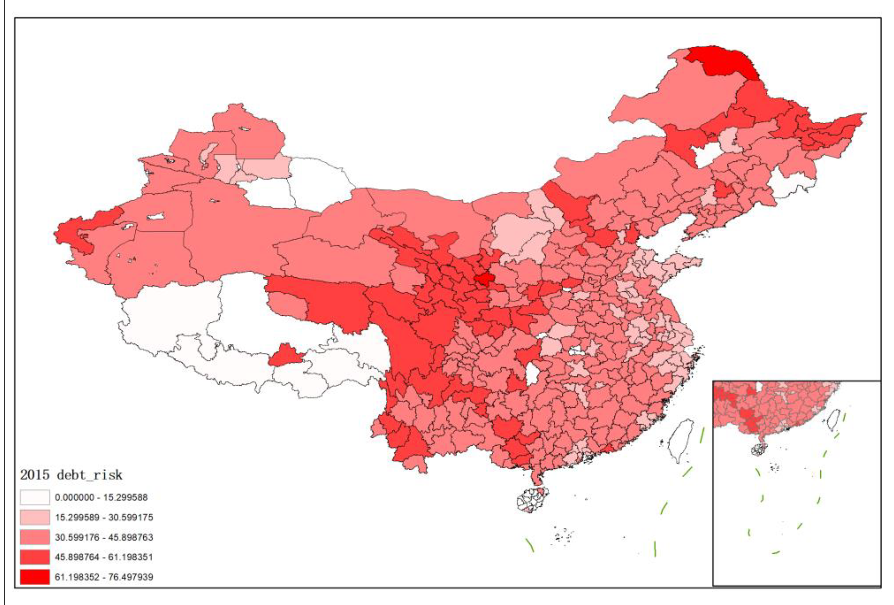
4.1.3. Risk Measurement Results

The obtained risk scores are as follows (the

Table 2. Estimation results of hidden debt risks of local government in some regions.

Hidden Debt Risk Score of Local Governments from 2015 to 2019
City	2015	2016	2017	2018	2019
DaLian	28.91195865	27.01909757	27.01909757	26.82933379	27.13279683
FoShan	24.88427547	20.69429354	21.00837985	20.68418926	22.80717264
GuiYang	35.82599862	41.29675679	42.89506015	43.58357522	46.21221067
HangZhou	22.31973813	22.68887937	23.97975023	24.96269211	25.67033526
HeFei	26.44453195	27.38022434	28.66337798	27.63176307	28.6051096
ChengDu	29.09142402	31.38266027	32.27327735	32.299866	33.69958921
NanJing	31.58680464	35.4738262	37.70630978	37.75690817	38.34087508
QingDao	22.63640076	23.48652464	23.96435764	24.89896249	25.40073198
XiaMen	20.56937056	21.98883352	21.86581334	22.43105817	22.51233708
WuHan	26.24344645	29.10143112	32.36544172	32.88963164	35.74540001
ChangSha	29.77736434	31.85709377	33.90888629	33.77429626	33.64897213
TaiYuan	36.81320446	36.99256896	37.21894672	35.06612106	36.15748302
YinChuan	30.97243077	31.59271035	31.80064509	32.68492259	34.39953412
ZhengZhou	24.82557524	27.16760343	30.26104457	31.36780589	31.92575389
ZunYi	36.95828029	39.5503283	41.18212671	43.50457706	44.21434143

contains only the calculation results of some prefecture-level cities).

Judging from the calculation results, the risk value of hidden debt in most regions from 2015 to 2019 has shown an increasing trend, and the risk value of different regions has a certain difference.

The hidden debt risks of local governments are presented using the map in Figure 1 using Arcmap software. We take the 2015 data as an example.

Excluding the areas with missing data, there were 337 prefecture-level administrative units with observable hidden debt risks in China in 2015. It can be seen that the implicit debt risk scores of various prefecture-level administrative regions are mostly in the range from 30 to 45, indicating that the overall risk is controllable. At the same time, from the perspective of spatial distribution, debt risk presents certain characteristics of “high-high” and “low-low” aggregation, among which the central, western, and northeastern regions of China and individual prefecture-level administrative regions in the western border show relatively high level of risk, while many prefecture-level administrative regions in southwest Tibet are at the lowest level of debt risk.

4.2. Systemic Financial Risks Measurement

4.2.1. Model Selection and Indicator System Construction

This paper uses the CRITIC-TOPSIS method when calculating systemic financial risk. When selecting the evaluation indices for measuring risk, on the one hand, the study by Wei Jinming, 2016 [42] is referred to. On the other hand, the data validity and availability are taken into account. The evaluation indicators selected are shown in

Table 3. Systemic financial risk measurement indicators.

Index Name	Calculation Method	Indicators Category
A bank’s equity to debt ratio	Owner’s equity/the total amount of liabilities	Negative
Income ratio on bank assets	Earnings before interest and tax/the total assets	Negative
Bank loan provision ratio	Loss reserve balance/loan balance	Negative
Foreign exchange deposit growth ratio of local banks	Increase in foreign exchange deposits/balance of previous period	Negative
Local GDP growth rate	Local GDP value added/GDP of the previous period	Negative
Local government expenditure growth ratio	Increase in government expenditure/expenditure of the previous period	Positive
Local government revenue growth ratio	Increase in government revenue/revenue in the previous period	Negative
The depth of the insurance	The premium income/the local GDP	Negative
The density of insurance	The premium income/population of prefecture-level cities	Negative
Premium income growth ratio	Premium Income appreciation/stock of premium income for the previous period	Negative
House price growth ratio	Increase in house price/house price for the previous period	Positive
Registered urban unemployment rate	Number of registered unemployed in urban areas/(number of urban employees + the number of registered unemployed in urban areas which was actually recorded)	Positive
Growth rate of foreign investment	Increase in actual foreign investment/investment in previous period	Negative
Debt to assets ratio	Total liabilities of enterprises above designated size/total assets	Positive
Rate of profit growth	The increase in profits of enterprises above designated size/profit of previous period	Negative

below.

4.2.2. Analysis of Measurement Results

The risk scores obtained are as follows (

Table 4. Measurement results of systemic financial risks in some regions.

Local Systemic Financial Risks Score from 2015 to 2019
City	2015	2016	2017	2018	2019
ChangZhou	38.20756056	42.30275228	28.98779277	24.45106123	27.48464988
ChaoYang	89.56932006	69.98286175	65.83319308	41.31064849	60.90540575
ChengDu	33.55807298	53.64490021	22.94075988	29.17260199	9.368536512
DaLian	78.09844909	26.22328099	11.48458561	26.1926513	31.14410454
DeYang	45.42555018	42.33301124	44.59671256	22.16285414	43.36796506
GuangZhou	25.74234059	41.50747432	19.74169279	25.19470724	33.14337413
QingDao	25.19847995	31.98539797	32.47204164	39.23882547	26.02047333
WeiHai	29.9857466	33.16174856	25.84446234	56.07923056	28.32955548
WuHan	25.76591622	31.63427358	20.49237223	18.02283144	20.90894899
XiAn	12.12126201	17.45043196	4.782075525	14.65546229	14.15206846
ChangChun	42.45182789	34.73496561	40.09737321	35.33977111	27.02704911
ZhuHai	24.17845354	24.22689292	34.67281304	17.42236564	20.52817343
HangZhou	15.37049824	25.03725261	14.01116599	8.260911013	21.37019523
NanJing	20.11287882	19.11042375	36.56750808	18.34679802	37.53503965
FuXin	100	70.26313263	56.41968825	52.7655466	66.54459868

only contains the measurement results of some prefecture-level cities).

From the calculation results, we can see that there is a large gap in the systemic financial risks in different regions, and the fluctuation trend of systemic financial risks in different regions is not very different, indicating that there are significant differences in the financial risk prevention and control capabilities of different regions.

At the same time, in order to meet the needs of early risk warning, based on the systemic financial risks score and according to the [0%, 33%], [34%, 66%], [67%, 100%] interval segments, systemic financial risks are divided into three types of risk early warning states. That is, the score ∈ [0, 33] is divided into risk low warning, the score ∈ [34, 66] is the risk middle warning, and the score ∈ [67, 100] is the risk high warning.

5. Research Design

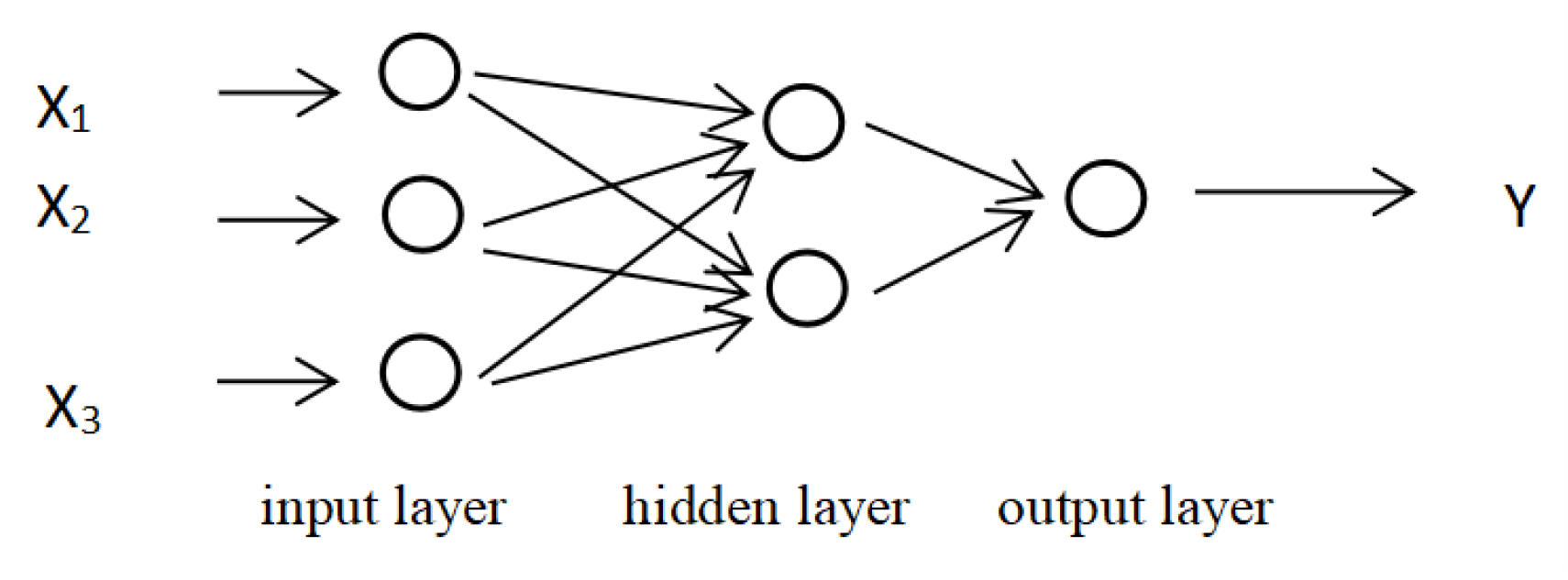
5.1. Introduction to BP Neural Network Model

BP neural network is a type of artificial neural network, and it is one of the most widely used neural networks in various fields of academic research. In 1986, the BP neural network was proposed by a scientific group represented by Rumeihart and McClelland, who generalized it as a feedforward network trained according to the error back propagation algorithm.

Drawing on the introduction of neural networks by Rumelhart et al. (1986) [43], the BP neural network consists of three parts: input layer, hidden layer, and output layer. Each layer structure has different neurons, and neurons in different layers are connected to each other. The original index data onto the research object is input from the input layer, and the hidden layer in the middle position realizes nonlinear processing on the input of the input layer node through the activation function, thereby connecting the input layer and the output layer of the network, and the obtained result is finally output by the output layer. If the input layer of the BP neural network has three neurons, the hidden layer has two neurons and only one layer, the output layer has one neuron, and the BP neural network is obtained in Figure 2.

The learning algorithm of the BP neural network model includes forward propagation to obtain the output layer error, according to the expected value and the error obtained from the output layer to judge whether to carry out back propagation. If the error is not reduced to the range of the pre-set value range, we carry out the error inversion. Then, the weights and thresholds between layers are continuously revised, and the training is stopped when the error is reduced to a predetermined value range.

The forward propagation process includes inputting the vector matrix X of the independent variable from the input end and adjusting the vector matrix of the input layer through the weight (W₁) and the threshold (b₁) to obtain the input Z₁ at the hidden layer end. The formula is as follows.

Z₁ = X*W₁ + b₁

(1)

Select an appropriate activation function in the hidden layer (f₁ is the activation function from the input layer to the hidden layer) to activate Z₁ to obtain A₁. The formula is as follows.

A₁ = f₁(Z₁)

(2)

After A₁ is adjusted by the weight (W₂) and the threshold (b₂), Z₂ is obtained. The formula is as follows.

Z₂ = A₁*W₂ + b₂

(3)

In the transmission from the hidden layer to the output layer, we select an appropriate activation function (f₂ is the activation function from the hidden layer to the output layer) to activate Z₂, and obtain the output layer estimated value A₂. The formula is as follows.

$$\widehat{Y} = {\mathrm{A}}_2 = {\mathrm{f}}_2\left({\mathrm{Z}}_2\right)$$

(4)

After comparing the estimated value of the output layer with the real value, the loss is calculated according to the loss function to determine whether to carry out error back propagation. The gradient descent method is commonly used in backpropagation. The principle is to randomly assign weights and thresholds to the weights and thresholds. After calculating the error, the output layer is reversely derived. In autonomous learning, the weights and thresholds are changed according to the gradient direction. The process iterates continuously until the output error value can be within the preset error range, then stops the iteration, and selects the weight and threshold at this time as the most suitable point to save.

5.2. Index System Construction and Data Processing

5.2.1. Determination of Explanatory Variables and Explained Variables

This paper studies the contagion of local government implicit debts to systemic financial risks, and on this basis carries out early risk warning. Therefore, in

Table 5. Core explanatory variables and explained variable indicators.

		Variable Symbol	Variable Name
Explained Variable		fr_topsis	The level of systemic financial risk
Core explanatory variables	Macro core explanatory variables	dr_topsis	The level of hidden debt risks of local governments
	Micro core explanatory variables	platform	Scale of financing platform bank debt
		bond	Scale of urban investment bonds
		PPP	Scale of PPP

, the systemic financial risk (fr_topsis) is selected as the explained variable, and the implicit debt risk of local governments (dr_topsis) is the core explanatory variable at the macro level. In order to distinguish it from previous early warning studies that mostly use macroeconomic variables, this paper gradually introduces PPP project scale (PPP), financing platform bank debt scale (platform), and urban investment bond scale (bond) as the core explanatory variables at the micro level in the research to study whether each micro-indicator has an impact on systemic financial risk, so as to optimize the risk early warning model. Due to the lack of data on the scale of government guidance funds, which is not conducive to model training, it is not included in this study.

In addition, referring to Chen Shoudong et al. (2020) [44], the factors affecting systemic financial risk are constructed from three aspects: financial environment, real economy, and economic participants. The indicators are selected as the control explanatory variables in

Table 6. Control explanatory variables.

Variable Symbol	Variable Name	Variable Definitions
X1	GDP per capita	GDP/total population of the region
X2	Loan-to-deposit ratio	RMB loans/RMB deposits
X3	Economic openness	total import and export/GDP
X4	Proportion of real estate development investment	real estate development investment/GDP
X5	Urbanization level	urban population/total population
X6	Proportion of retail sales of social consumer goods	retail sales of social consumer goods/GDP
X7	Proportion of fixed asset investment	total fixed asset investment/GDP
X8	Urban basic education level	—
X9	The proportion of value-added in secondary production	secondary industry added value/GDP
X10	Population density	population/land area

.

5.2.2. Data Sources and Data Processing

The data in this paper are mainly collected through Wind database, China Economic Net, government PPP project database, enterprise early warning, private equity, and statistical yearbook.

This paper selects the data of cities in China from 2015 to 2019. After eliminating the prefecture-level cities with missing data and processing outliers, 970 samples were finally left, with a total of 194 prefecture-level cities.

5.3. BP Neural Network Model Optimization

5.3.1. Input and Output Data Preprocessing

First of all, for the needs of financial risk early warning, the data of prefecture-level cities from 2015 to 2018 (80% of all samples) are used as the training set for the study, and the data of prefecture-level cities in 2019 (20% of all samples) are used as a test set.

Then, we normalize the input and output data. On the one hand, it can make the model converge faster, and on the other hand, it can also meet the requirements of the activation function of the neural network for the value range, that is, it is limited to the range of [0, 1]. The specific formula of the normalization method in this paper is as follows.

y_i = (x_i − x_min)/(x_max − x_min)

(5)

Among it, y_i represents the data processed by this method, x_i represents a certain data of the input indicator, x_min represents the minimum data value of the indicator, and x_max represents the maximum data value of the indicator. The index data of the input layer and the output layer are normalized by the normalization function mapminmax in Matlab20a.

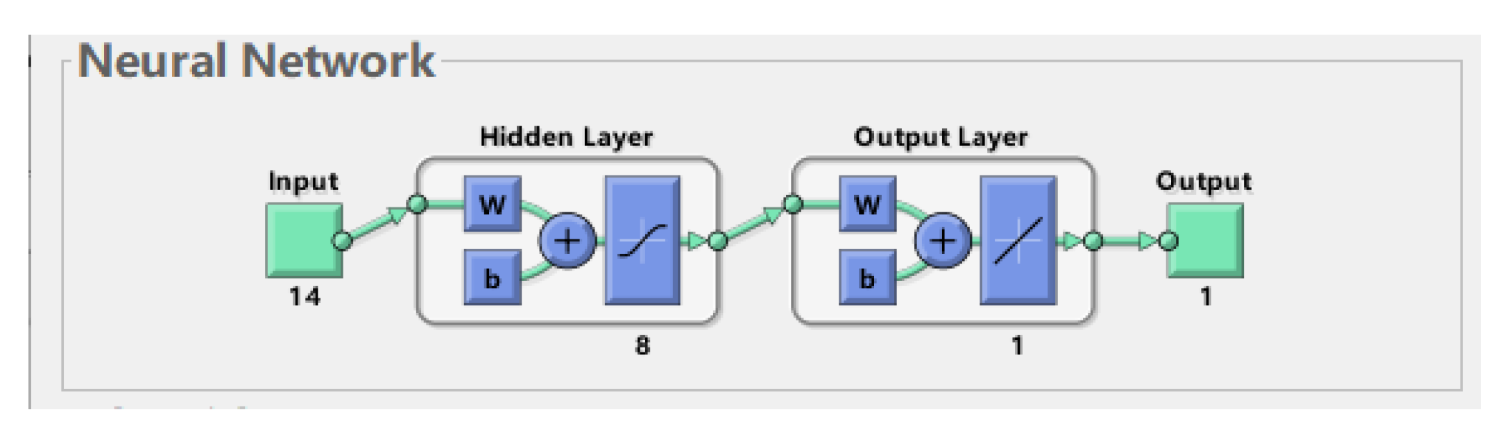
5.3.2. BP Neural Network Structure Design

In the process of designing the structure of the neural network, Li Lizhen (2021) [45], Yan Peiyu (2018) [46], and Wu Wenqian (2020) [47] set the number of network layers, network nodes, activation functions, training methods, and parameters of the BP neural network. The design process of this article is as follows.

1. Setting the number of network layers.

The BP neural network has three parts: input layer, hidden layer, and output layer. The higher the number of network layers, the better the neural network training effect will be from a theoretical point of view. However, deepening the number of network layers may lead to over-fitting problems and increase the difficulty of model fitting. Therefore, in the selection of the number of network layers, on the one hand, we draw lessons from the setting of the model structure in the previous research (Wu Wenqian (2020) [47]), and on the other hand, we constantly deepen the number of layers to compare the model training effect. When the number of layers of the hidden layer is 1, the training effect of the model is the best.

2. Setting the number of network nodes.

In this paper, the input layer inputs explanatory variables, and the output layer outputs an explained variable, so the number of nodes in the input layer is set as the number of explanatory variables, and the number of nodes in the output layer is 1.

The setting of the number of hidden layer nodes is the key to model training, which has a great impact on the performance of the BP neural network. Generally speaking, the more the number of hidden layer nodes is set, the better the performance will be that can be brought to the network. However, at the same time there may be an overfitting problem. Therefore, in terms of the setting of hidden layer nodes, an empirical formula is used to give a setting range of the number of nodes, and then the optimal number of hidden layer nodes is found through repeated network training. The empirical formula is as follows:

$$\left(1\right) \mathrm{m}=\sqrt{\mathrm{n}+\mathrm{l}}+\propto ,$$

(6)

$$\left(2\right) \mathrm{m}={\log }_2\mathrm{n},$$

(7)

$$\left(3\right) \mathrm{m}=\sqrt{nl}.$$

(8)

Among them, m represents the number of hidden layer nodes, n represents the number of input layer nodes, l represents the number of output layer nodes, and ∝ represents a constant from 1 to 10. According to the empirical formula, the value range of the number of hidden layer nodes can be obtained, and then the size of m is adjusted in turn during the training process to obtain the number of hidden layer nodes when the training performance is the best.

3. Activation function selection of the neural network.

The activation function is an important part of building a neural network. It operates between neurons in different layers of the network structure, and it determines whether a neuron is activated. The activation function mainly maps the input of the upper layer node to the output, realizes the nonlinear transformation of the input value, and makes the network approximate any nonlinear function, so as to explore the nonlinear relationship between the input layer and the output layer indicators. In the existing research, the widely used activation functions are the Tan-sigmoid function, the Log-sigmoid function, and the Purelin function. Generally, according to the data characteristics of the research object, by drawing on the existing research of scholars and continuous trial and error through model training, the activation function that makes the best model training has been chosen. The activation function from the input layer to the hidden layer in this paper is the Tan-sigmoid function. It can map the data interval to (0, 1), and the formula is as follows:

$$\tan \mathrm{sig}\left(\mathrm{x}\right)=\frac{2}{1+{\mathrm{e}}^{-2\mathrm{x}}}-1 .$$

(9)

The activation function from the hidden layer to the output layer is the Purelin function, which is a linear function.

4. Selection of the training method of the neural network.

The initial training method of the BP neural network is the gradient descent method. The Levenberg–Marquardt algorithm is the most common nonlinear least squares algorithm used so far. It uses a gradient to find the maximum value as an optimization algorithm. In this paper, when selecting the training method, based on the advantage of the LM algorithm’s faster optimization speed, combined with the characteristics of the research data, the LM algorithm is selected as the optimization algorithm of the gradient descent method for model training.

5. Parameter design of the neural network.

When choosing different parameters, on the one hand, we refer to the settings of the network parameters that have been studied, and on the other hand, we adjust the network training constantly to compare the training efficiency under different parameters. Finally, we set the model to have 5000 iterations, the learning accuracy to 0.01, and the learning rate to 0.01.

5.3.3. Comparative Analysis of the Results of Different BP Neural Network Models

This paper first introduces the implicit debt risk at the macro level into the neural network, and then introduces three indicators at the micro level in turn: PPP project scale (PPP), financing platform bank debt scale (platform), and urban investment bond scale (bond). We explore whether micro-level indicators have an impact on financial risks, and through comparative analysis, we get the best explanatory variable selection for model training. The results are placed in

Table 7. Comparison of the training effects of adding explanatory variables in turn.

Core Explanatory Variables	MSE	Training:R	Validation:R	Test:R	ALL:R
dr_topsis	0.0115	0.63208	0.54175	0.51753	0.59908
dr_topsis, PPP	0.0108	0.67956	0.58974	0.55209	0.64012
dr_topsis, PPP, platform	0.00994	0.74429	0.61186	0.49528	0.68938
dr_topsis, PPP, platform, bond	0.00976	0.7572	0.59618	0.69377	0.71284

.

It can be seen that when the core explanatory variable only has macroscopic implicit debt risk, the error of the neural network model is 0.0115, and the overall goodness of fit (R) is only 0.59908. After adding the three indicators of PPP project scale, financing platform bank debt scale, and urban investment bond issuance scale in turn, the mean square error (MSE) is gradually decreasing, and the goodness of fit of the model is gradually increasing. It shows that the three microscopic explanatory variables introduced in this paper all have a certain impact on systemic financial risk, and they also need to be introduced in the risk early warning model.

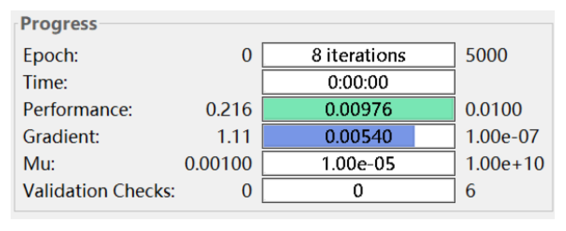
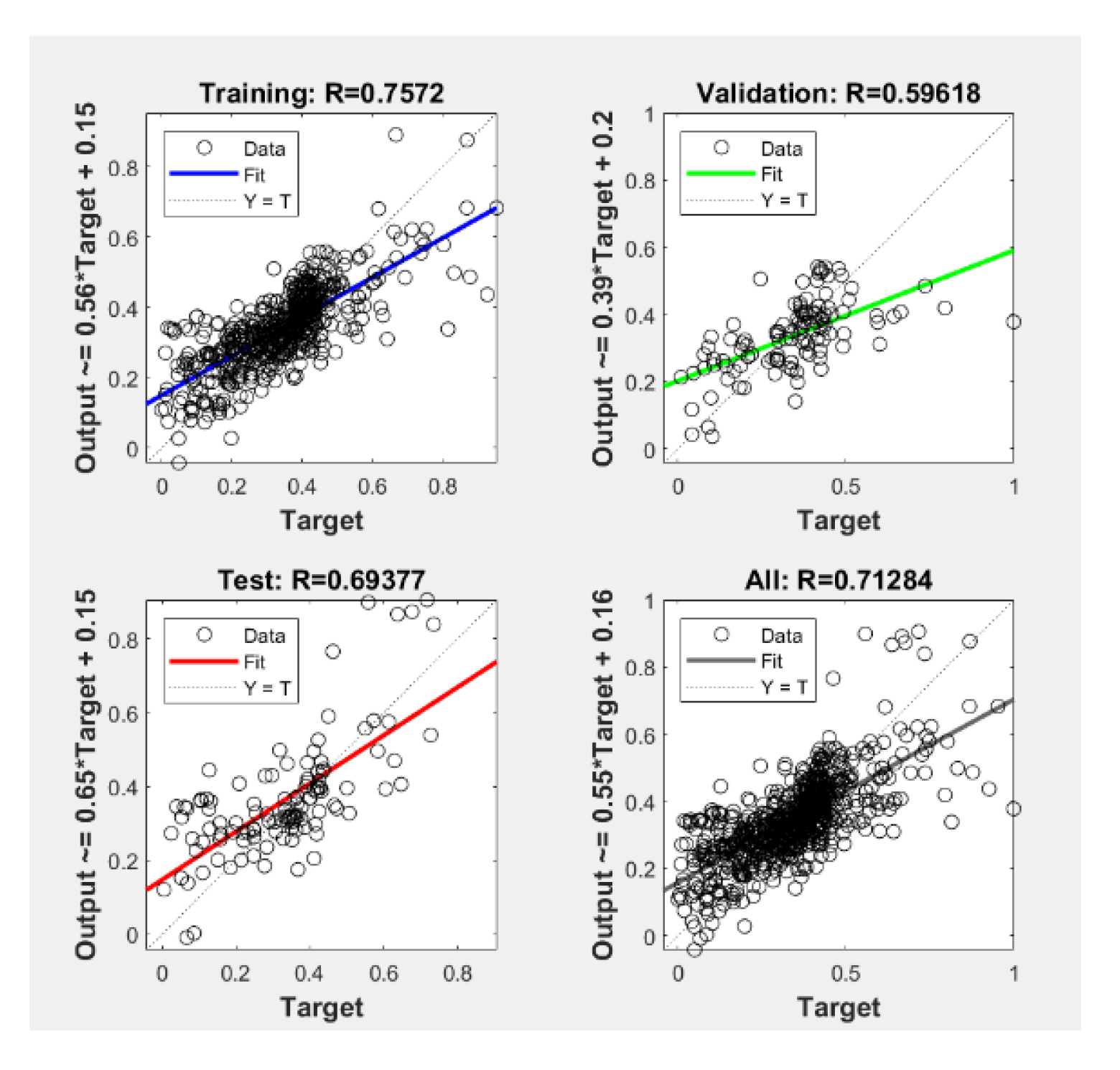
5.4. Analysis of Training Results of BP Neural Network Model

Based on the above analysis, when the core explanatory variables include the four core explanatory variables: implicit debt risk, PPP scale, financing platform bank debt scale, and urban investment bond scale, the neural network training effect is the best, so the risk early warning model introduces the above four core explanatory variables simultaneously. The model is trained by Matlab2020a, in Figure 3, the input layer has 14 neurons, the output layer has 1 neuron, the network contains a hidden layer, and the hidden layer has 8 neurons.

The results of the BP neural network model training are in Figure 4. After eight iterations of the model, the MSE (mean square error) of the model is less than the preset learning accuracy of 0.01, and the model training ends.

$$MSE=\frac{1}{n} {\sum }_{i=1}^n{W}_i{\left(y_i-{\widehat{y}}_i\right)}^2.$$

(10)

It can be seen from the training results of the neural network that the network performance is good. After eight iterations, the MSE drops to the preset learning accuracy, and the MSE is 0.00976. From the regression of the neural network in Figure 5, it can be seen that the overall goodness of fit (R value) is 7.13 × 10⁻¹, the goodness of fit of the training set is7.57 × 10⁻¹, and the goodness of fit of the test set is 6.94 × 10⁻¹. Most of the data can be concentrated around the fitted function, which means that the neural network is well trained.

6. Analysis of Early Warning of Systemic Financial Risks

6.1. Risk Contagion Effect Analysis

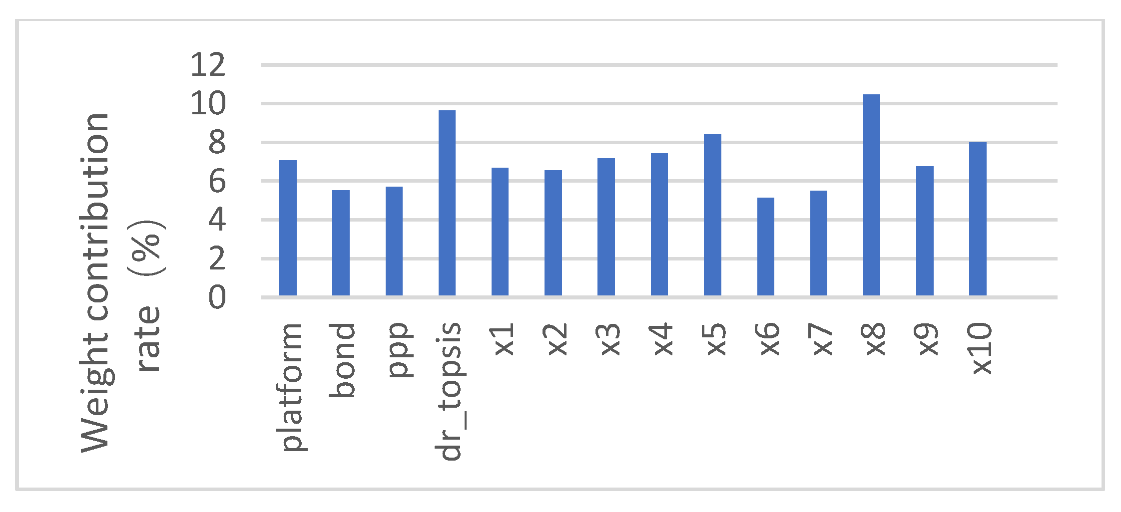
6.1.1. The Weight Contribution Rate of the Input Node

In the process of studying the contagion effect of local government implicit debt on systemic financial risks, after storing the weights and thresholds of the trained network, the input layer of BP neural network is calculated by referring to the factor weight analysis method used by Li Zuoyong et al. (2004) [48]. The weight analysis of factors refers to calculating the proportion of the connection weights of the neurons connected to the input factors to the total connection weights of all neurons in the input layer, so as to obtain the contribution ratio of different input factors to the output factors. The effect of the explanatory variables on the explanatory variables is determined by comparing the weight contribution rate of the different input factors to the output factors. The expression of the contribution rate of different input index weights is:

$$b_i={\sum }_i\left|W_{ij}\right|·[\left|V_j\right|·\left(\ln \left|W_{ij}\right|/\ln {\sum }_i\left|W_{ij}\right|\right)].$$

(11)

In the above formula, $W_{ij}$ is the weight of the input index i to the hidden layer node j, and $V_j$ is the weight between the hidden layer node j and the output node. The weight contribution rate of the input index i subjected to the normalization process is:

$$c_i=b_i/{\sum }_i{b}_i.$$

(12)

The calculated explanatory variable factor weight contribution rate is in

Table 8. Weight contribution rate of explanatory variables.

Explanatory Variable Symbols	Weight Contribution Rate (%)	Explanatory Variable Name
platform	7.06017419973742	Scale of financing platform bank debt
bond	5.5089920219434	Scale of urban investment bonds
ppp	5.7141804836627	Scale of PPP
dr_topsis	9.63355766336391	The level of hidden debt risks of local governments
x1	6.67543190738213	GDP per capita
x2	6.53953061839073	Loan-to-deposit ratio
x3	7.17573766322704	Economic openness
x4	7.41645669864381	Proportion of real estate development investment
x5	8.40474594921744	Urbanization level
x6	5.14368458380196	Proportion of retail sales of social consumer goods
x7	5.48470869969032	Proportion of fixed asset investment
x8	10.4681165059406	Urban basic education level
x9	6.75215545564988	The proportion of value added in secondary production
x10	8.0225275493487	Population density

.

6.1.2. Analysis of Explanatory Variable Importance

Referring to the factor weight analysis method, the histogram of the weight contribution rate of different explanatory variables is obtained in Figure 6.

As the results shown in Figure 6, the higher the weight contribution rate column, the greater the weight contribution rate of the variable, and the greater the influence of the explanatory variable on the explained variable. After sorting the weight contribution rate of explanatory variables, we can see that the weight contribution rate of local government implicit debt risk to systemic financial risk is 9.63%, which is higher than the weight contribution rate of most other explanatory variables to systemic financial risk. It shows that among the many influencing factors, the implicit debt risk of local governments has a greater impact on systemic financial risk. On a micro level, the scale of financing platform bank debt has the greatest impact on systemic financial risk, and the scale of PPP and urban investment bonds also have a certain degree of impact on systemic financial risk.

In general, both macro and micro variables of local government implicit debt will have a greater impact on systemic financial risks, which also shows that local governments borrow debt through financing platforms, issue urban investment bonds, or invest in PPPs, which can infect systemic financial risk.

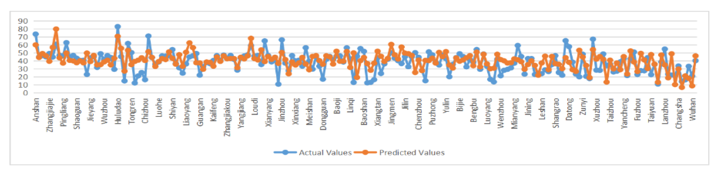
6.2. Risk Early Warning Analysis

After the BP neural network is trained, the model can be applied to the early warning study of systemic financial risk. The test set of this paper is the prefecture-level city data of 2019, and after the data input of the previous four years is better trained and the weights and thresholds are saved, the systemic financial risk data of 2019 is then predicted. The risk prediction effect is then tested by comparing its predicted value with the actual value to achieve the purpose of risk early warning.

Through the simulation test code and inverse normalization code in MATLAB, the actual value of systemic financial risk is compared with the predicted value output by network training, and the comparison figure is as follows:

It can be seen that most of the predicted values of the test set can be better approximated to the actual values. Combined with the fitting results obtained from the training model (the goodness of fit is 0.69377), it shows that there is some reliability in predicting systemic financial risk using the constructed and trained BP neural network model. That is, when the relevant indicators of local government hidden debt risk are signaled, the systemic financial risk can be predicted by the neural network, which plays a certain role in the early warning of systemic financial risk.

From the comparison between the systematic financial risks prediction results and the true value of the prefecture-level cities (Figure 7), it can be seen that the relative error between most of the prediction results and the true values is controlled within ±20%, indicating that the BP neural network financial risks early warning system constructed in this paper has a good early warning effect and has certain reference significance for a local government to carry out financial risks warning. At the same time, in view of the risk states of the predicted systemic financial risks of prefecture-level cities (“low warning”, “middle warning”, and “high warning”) (

Table 9. Comparison of predicted and actual values of test sets for some prefecture-level cities.

City	Heihe	Wuzhong	Tonghua	Huludao	Yueyang	Weihai	Huzhou	Fuzhou	Yibin
Actual Values	44.81	44.91	44.69	82.90	44.87	28.33	17.77	22.85	40.52
Predicted Values	44.22	46.32	56.81	70.69	46.53	31.38	18.98	26.59	40.03
Relative Error	−1%	3%	27%	−15%	4%	11%	7%	16%	−1%
Risk State	Middle Warning	Middle Warning	Middle Warning	High Warning	Middle Warning	Low Warning	Low Warning	Low Warning	Middle Warning

), a local government can take targeted preventive measures to achieve a more targeted purpose of preventing systemic financial risks.

6.3. Early Warning Stress Test

The early warning stress test is used to examine the early warning situation of systemic financial risks after training and testing the constructed BP neural network. The test set data in the simulation model are in different stress states. In this paper, the scale of financing platform bank debt, the scale of urban investment bonds, the scale of PPP, and the level of hidden debt risk are within a relatively large stress range: an increase of 10% (mild stress), 20% (moderate stress), and 30% (severe stress). The changes in systemic financial risks are obtained as follows (

Table 10. Stress test results (increase by 10%, 20%, and 30%).

		Platform (Change Value)	Bond (Change Value)	Ppp (Change Value)	Dr_Topsis (Change Value)	Fr_Topsis (Change Value)
Stress range	Mild stress	10%	10%	10%	10%	13.36%
		10%				1.06%
			10%			6.66%
				10%		1.97%
					10%	11.43%
	Moderate stress	20%	20%	20%	20%	18.41%
		20%				2.02%
			20%			4.16%
				20%		3.67%
					20%	20.23%
	Severe stress	30%	30%	30%	30%	22.87%
		30%				1.26%
			30%			4.44%
				30%		1.57%
					30%	19.14%

).

In general, when the implicit debt of local governments changes under different stress, the constructed neural network model can sensitively predict changes in systemic financial risks, and has a good early warning effect. When the four core explanatory variables increase by 10% at the same time, the level of systemic financial risk increases greatly. The average value increases by 13.36%. When it increases by 20%, the systemic financial risk value increases by 18.41%, and when it increases by 30%, the systemic financial risk value increases by 22.87%. When the hidden debt risk of local governments increased by 10%, 20%, and 30%, the systemic financial risk value increased by 11.43%, 20.23%, and 19.14%. Changes in the implicit debt stress of local governments will be significantly transmitted to systemic financial risks, which will have a greater negative impact on the stability of the financial system. Among the specific types of local government implicit debts, when the scale of urban investment bonds increases by 10%, 20%, and 30%, the systemic financial risk value increases by 6.66%, 4.16%, and 4.44%. When the PPP scale increases by 10%, 20%, and 30%, the systemic financial risk value increases by 1.97%, 3.67%, and 1.57%. When the scale of financing platform bank debt increases by 10%, 20%, and 30%, the systemic financial risk value increases by 1.06%, 2.02%, and 1.26%. Stress changes in the micro-variables of local government implicit debt will also be significantly transmitted to systemic financial risks.

7. Conclusions and Recommendations

7.1. Conclusions

This paper uses a micro-level local financing platform bank debt scale, urban investment bond scale, PPP scale, and macro-level local government implicit debt risk level as the core indicators of the input layer, and systemic financial risk as the output layer indicator, using a neural network model to study the contagion of local government implicit debt to systemic financial risk, and then use the trained model to give an early warning of systemic financial risk, and draw the following conclusions:

(1)

Local government hidden debt has a significant contagion effect on systemic financial risk. Among the many factors affecting systemic financial risk, macro indicators of local government hidden debt risk explain the systemic financial risk to a higher extent. The scale of financing platform bank debt at the micro level has a greater impact on systemic financial risk, and the scale of PPP and urban investment debt also have a certain degree of impact on systemic financial risk;

(2)

All categories of local government implicit debt indicators, including macro and micro levels, are the best early warnings of systemic financial risks. Through the training and testing of the BP neural network, the systemic financial risk at the prefecture-level city level can provide an early warning with a certain degree of reliability. That is, the signals from the data of relevant indicators of local government hidden debts can be used to provide an early warning of systemic financial risks in China through neural network models with high applicability;

(3)

When the implicit debt of local governments changes under different stress, the constructed neural network model can sensitively predict changes in systemic financial risks, which has a good early warning effect. When the level of hidden debt risk, the scale of financing platform bank debt, the scale of urban investment bonds, and the scale of PPP pressure changes simultaneously, or when the level of hidden debt risk and different types of micro-variables undergo stress changes independently, they will all significantly transmit to systemic financial risks. It has a large negative impact on the stability of the financial system.

7.2. Suggestions

In terms of macro regulation of local government hidden debt. A large-scale inspection of local governments’ hidden debts should be conducted to fully sort out local government’s sources of debt financing, debt maturity, and repayment, and to monitor the debt risk level in real time. At the same time, to strengthen the supervision of local government hidden debt and to further clarify the definition and classification of hidden debt, local governments should ‘do something and not do something’ to prevent the impact of China’s systemic financial risks.

In terms of micro regulation of different types of local governments’ hidden debts, first, whether it is local financial difficulties or the current impact of COVID-19 pandemic, the state should not relax the control of local governments through the financing platform irregular debt, the flow of funds, and the future repayment of local financing platform bank debt rectification and regulation, clear flow of funds, the development of a more reasonable debt borrowing and repayment mechanism. Secondly, the issuance of urban investment bonds should also realize more scientific information disclosure, monitor the flow of funds of urban investment bonds, and reasonably control the scale of urban investment bonds. Thirdly, due to the long cycle of PPP projects, the flow of government financial funds should be continuously monitored to reasonably match the government’s financial strength with the scale of PPP projects and strengthen the awareness of risk prevention under a stable infrastructure.

In terms of early warning of systemic financial risk based on local government implicit debt data, the neural network model constructed in this paper can be used to predict China’s future systemic financial risk based on macro and micro level local government hidden debt big data to achieve timely risk warning for local government hidden debt signals. At the same time, differentiated prevention and control measures have been adopted for different types of local government implicit debt risk conditions to effectively prevent systemic financial risks.

References

1. Wang, T.; Jin, H.; Zhu, J. Research on regional financial risks arising from local government debts and countermeasures. Inn. Mong. Financ. Res. 2012, 4, 38–40. [Google Scholar]
2. Harvey, S.R. Fiscal Science; People’s University of China Press: Beijing, China, 2002. [Google Scholar]
3. Brixi, H.P. Contingent Government Liabilities: Fiscal Threat to the Czech Republic? Post-Sov. Geogr. Econ. 2000, 41, 63–76. [Google Scholar] [CrossRef]
4. Ponds, E.; Severinson, C.; Yermo, J. Implicit Debt in Public-sector Pension Plans: An International Comparison. Int. Soc. Secur. Rev. 2012, 65, 75–101. [Google Scholar] [CrossRef]
5. Wenxiu, H.; Cheng, L. Potential and Sustainability of Active Fiscal Policy; Economic Science Press: Beijing, China, 2000; Chapter 4; pp. 62–81. [Google Scholar]
6. Shaobo, L.; Wenqing, H. Study on the status of local government hidden debt in China. Fisc. Res. 2008, 9, 64–68. [Google Scholar]
7. Moody. Public Finance-General Obligation Bonds Issued by U.S. Local Governments. Rat. Methodol. 2009, 7, 11–19. [Google Scholar]
8. Ming, Y. An analysis of local government hidden debt risk prevention—Based on information disclosure and full-caliber budget supervision. Financ. Account. Newsl. 2019, 35, 106–109. [Google Scholar]
9. Pabuçcu, H.; Ayan, T.Y. The development of an alternative method for the sovereign credit rating system based on adaptive neuro-fuzzy inference system. Am. J. Oper. Res. 2016, 7, 41–55. [Google Scholar] [CrossRef] [Green Version]
10. Sarlin, P. Sovereign debt monitor: A visual self-organizing maps approach. In Proceedings of the 2011 IEEE Symposium on Computational Intelligence for Financial Engineering and Economics (CIFEr), Paris, France, 11–15 April 2011; pp. 1–8. [Google Scholar]
11. Lehar, A. Measuring Systemic Risk: A Risk Management Approach. J. Bank. Financ. 2005, 29, 2577–2603. [Google Scholar] [CrossRef] [Green Version]
12. Matheson, T.D. Financial conditions indexes for the United States and euro area. Econ. Lett. 2012, 115, 441–446. [Google Scholar] [CrossRef]
13. Celik, S. The More Contagion Effect on Emerging Markets: The Evidence of DCC-GARCH Model. Econ. Model. 2012, 24, 1946–1959. [Google Scholar] [CrossRef]
14. Shoudong, C.; Dakun, Z.; Xianliang, C. Using binary choice model to establish a financial early warning model in China. Learn. Explor. 2006, 1, 237–239. [Google Scholar]
15. Shoudong, C.; Hui, M.; Chunzhou, M. MS-VAR model for financial risk early warning in China and the study of zone system state. J. Soc. Sci. Jilin Univ. 2009, 49, 110–119+160. [Google Scholar]
16. Mengyu, L. Research on the construction of financial risk early warning system in China based on K-mean clustering algorithm and BP neural network. J. Cent. Univ. Financ. Econ. 2012, 10, 25–30. [Google Scholar]
17. Yin, D.; Ziqing, M.; Tao, Z.; Dongfa, F. Progress in the application of big data methods in systemic financial risk monitoring and early warning. Financ. Dev. Res. 2022, 2, 3–12. [Google Scholar]
18. Sosa-Padilla, C. Sovereign defaults and banking crises. J. Monet. Econ. 2012, 99, 88–105. [Google Scholar] [CrossRef]
19. Gennaioli, N.; Martin, A.; Rossi, S. Sovereign default, domestic banks, and financial institutions. J. Financ. 2014, 69, 819–866. [Google Scholar] [CrossRef] [Green Version]
20. Magkonis, G.; Tsopanakis, A. The financial and fiscal stress interconnectedness: The case of G5 economies. Int. Rev. Financ. Anal. 2016, 46, 62–69. [Google Scholar] [CrossRef] [Green Version]
21. Silva, T.C.; Guerra, S.M.; Tabak, B.M. Fiscal risk and financial fragility. Emerg. Mark. Rev. 2020, 45, 100711. [Google Scholar] [CrossRef]
22. Zhengyao, W. Research on the Linkage between Fiscal Risk and Financial Risk in China during the Transition Period; Southwest University of Finance and Economics: Chengdu, China, 2006; p. 212. [Google Scholar]
23. Shucai, M.; Xia, H.; Yunhong, H. The transmission mechanism of local government debt affecting financial risk--a study based on the perspective of real estate market and commercial banks. Financ. Forum 2020, 25, 70–80. [Google Scholar]
24. Xudong, Z. Local Government Debt and Regional Financial Risks; Lanzhou University: Lanzhou, China, 2021; p. 51. [Google Scholar]
25. Kotlikoff, L. Is the United States Bankrupt? Fed. Reserve Bank St. Louis Rev. 2006, 88, 235–249. [Google Scholar] [CrossRef] [Green Version]
26. Moro, B. Lessons from the European economic and financial great crisis: A survey. Eur. J. Political Econ. 2014, 34, S9–S24. [Google Scholar] [CrossRef]
27. Sibbertsen, P.; Wegener, C.; Basse, T. Testing for a break in the persistence in yield spreads of EMU government bonds. J. Bank. Financ. 2014, 41, 109–118. [Google Scholar] [CrossRef] [Green Version]
28. Ludwig, A. Credit risk-free sovereign bonds under Solvency II: A cointegration analysis with consistently estimated structural breaks. Appl. Financ. Econ. 2014, 24, 811–823. [Google Scholar] [CrossRef]
29. Gruppe, M.; Lange, C. Spain and the European sovereign debt crisis. Eur. J. Political Econ. 2014, 34, S3–S8. [Google Scholar] [CrossRef]
30. Basse, T.; Wegener, C.; Kunze, F. Government bond yields in Germany and Spain—Empirical evidence from better days. Quant. Financ. 2018, 18, 827–835. [Google Scholar] [CrossRef]
31. Hsing, Y. Determinants of the government bond yield in Spain: A loanable funds model. Int. J. Financ. Stud. 2015, 3, 342–350. [Google Scholar] [CrossRef] [Green Version]
32. Aizenman, J. The eurozone crisis: Muddling through on the way to a more perfect euro union? Soc. Sci. 2013, 2, 221–233. [Google Scholar] [CrossRef] [Green Version]
33. Merrick, J.J., Jr. Crisis dynamics of implied default recovery ratios: Evidence from Russia and Argentina. J. Bank. Financ. 2001, 25, 1921–1939. [Google Scholar] [CrossRef] [Green Version]
34. Hébert, B.; Schreger, J. The costs of sovereign default: Evidence from Argentina. Am. Econ. Rev. 2017, 107, 3119–3145. [Google Scholar] [CrossRef]
35. Feng, X. Local government debt and municipal bonds in China: Problems and a framework of rules. Cph. J. Asian Stud. 2013, 31, 23–53. [Google Scholar] [CrossRef] [Green Version]
36. Zhenhua, M.; Haixia, Y.; Xinhe, L.; Qiufeng, W.; Yuanhui, W. Analysis of current local government debt risk and transformation of financing platform in China. Fisc. Sci. 2018, 5, 24–43. [Google Scholar]
37. Ben, Y.; Yanjin, L.; Shengyin, O.; Shourong, M. Statistical Accounting and Causal Analysis of Local Hidden Debt Scale. Financ. Theory Pract. 2022, 43, 95–103. [Google Scholar]
38. Diakoulaki, D.; Mavrotas, G.; Papayannakis, L. Determining objective weights in multiple criteria problems: The critic method. Comput. Oper. Res. 1995, 22, 763–770. [Google Scholar] [CrossRef]
39. Hwang, C.L.; Yoon, K. Methods for multiple attribute decision making. In Multiple Attribute Decision Making; Springer: Berlin/Heidelberg, Germany, 1981; pp. 58–191. [Google Scholar]
40. Huaidong, Y.; Shuyue, C. Term mismatch, shadow banking interest rates and local government implicit debt risk. Wuhan Financ. 2021, 10, 35–42+77. [Google Scholar]
41. Zhenyi, X. Local Government Hidden Debt Risk Measurement and the Contagion Effect on Systemic Financial Risk; Sichuan University: Chengdu, China, 2021; p. 77. [Google Scholar]
42. Jinming, W. The measurement and influencing factors of systemic financial risk. Bus. Res. 2016, 2, 73–80. [Google Scholar]
43. Rumelhart, D.E.; Hinton, G.E.; Williams, R.J. Learning Representations by Back-propagating Errors. Nature 1986, 323, 533–536. [Google Scholar] [CrossRef]
44. Shoudong, C.; Zhuo, L.; Sihan, L. The spatial spillover effect of local government debt risk on regional financial risk. J. Xi’an Jiaotong Univ. Soc. Sci. Ed. 2020, 40, 33–44. [Google Scholar]
45. Lizhen, L. Research on the construction and application of local government contingent hidden debt risk early warning system--based on BP neural network analysis method. Financ. Econ. Ser. 2021, 3, 14–25. [Google Scholar]
46. Peiyu, Y. Research on the Impact of Two-Child Policy on China’s Population Structure Based on BP Neural Network; Qingdao University: Quingdao, China, 2018; p. 44. [Google Scholar]
47. Wenqian, W. Research on Factors Influencing Credit Spreads of Real Estate Enterprises’ Bonds Based on BP Neural Network Model; Shanghai University of Finance and Economics: Shanghai, China, 2020; p. 50. [Google Scholar]
48. Zuoyong, L.; Hengkang, D.; Jing, D. BP network weighting analysis model for atmospheric particulate matter source analysis. J. Sichuan Univ. Nat. Sci. Ed. 2004, 5, 1026–1029. [Google Scholar]
Figure 1. The value–at–risk of local government implicit debt risk.
Systems 10 00207 g001
Figure 2. Three-layer BP neural network structure.
Systems 10 00207 g002
Figure 3. BP neural network structure.
Systems 10 00207 g003
Figure 4. BP neural network training results.
Systems 10 00207 g004
Figure 5. Regression analysis of BP neural network.
Systems 10 00207 g005
Figure 6. Histogram of the weight contribution rate of the explanatory factors.
Systems 10 00207 g006
Figure 7. Comparison of the actual and predicted values of systemic financial risk values for prefecture-level cities in 2019.
Systems 10 00207 g007