1. Introduction
Teachers have to constantly estimate the probable effect of their decisions on the long-term learning achieved by their students. For each learning objective of the national curriculum, teachers have to make the students practice enough exercises. A key decision they must make is between asking students to perform exercises more carefully or perform more exercises. Thus, every month, teachers face the dilemma of what and how many exercises their students should practice, and what their consequences are on long-term learning. For that, they need to have a good prediction mechanism. This dilemma presents several challenges.
First, the mechanism should predict their students’ long-term learning. This is not straightforward because long-term learning is not always the same as short-term learning [
1]. Long-term learning is the learning evaluated at the end of the year, while short-term learning is learning evaluated during the session. This is a well-known, unintuitive phenomenon, where fast progress measured on real time generates an illusion of mastery in the students [
2,
3]. This illusion makes it difficult for the teachers to make a good prediction of the long-term learning of each of their students. Second, we must consider that teachers prefer to design their own questions. This generates a huge diversity and number of questions, each answered by very few students. Therefore, the data gathered are not suitable for typical big-data mining, such as deep learning algorithms. For example, Ref. [
4] found that logistic regression leads to data sets of a moderate size, whereas deep knowledge tracing leads to data sets of a large size.
Third, from one month to the next, teachers need a simple update mechanism. For example, they could use the average score on the answers to questions posed on the current month and an accumulative score of the previous months. There is no need for the whole history of scores of all answers to previous questions. The mechanism must also combine in a simple way, hopefully additively, with information on other personal attributes of students, their class and their school. These are personal attributes, such as student beliefs, course attributes, such as classroom climate, and school attributes, such as its historical performance on national standardized tests.
Fourth, the mechanism should facilitate simulating different practice strategies for the coming months. These strategies, together with the assessment in the current month, should be enough to predict the effect on the long-term learning. Teachers normally use grade point average (GPA) for this purpose. GPAs are very simple to understand. They are just averages of partial grades obtained across the year. Teachers could welcome a better predictor of long-term learning if it is as simple and interpretable as GPAs. However, they do not consider all the exercises performed by the students. There is also no evidence of its predictive power. If we were to use nonlinear models for this prediction, such as gradient boosted machines, k-nearest neighbors or random forests, this goal would not be possible. Non-linear intertwined relationship between the estimated model parameters and the predicted score are difficult to interpret. Most machine learning models are designed with features and combinations of them that maximize prediction performance. There is no consideration to generate solutions that are meaningful to domain experts, such as teachers [
5]. They are typically black boxes that are not transparent to users [
6]. However, interpretability is critical for teachers to adopt the model, to simulate instructional strategies to follow in the coming months, and to use them to base their decisions.
Therefore, in order to improve the quality of education, teachers need to be able to predict for each student her long-term learning and how different strategies can impact this prediction. One way to do so is to know the current state of long-term learning of each student, and how different strategies could interact with each student’s current state. Thus, based on an estimation of the actual state of long-term learning of each student and the effects of different strategies that actuate on the current state of each student, the teacher has to adjust her strategies of exercise practice in order to reach a specified long-term learning target.
3. Theoretical Framework
An important part of the learning challenge of school mathematics is due to an evolutionary mismatch or evolutionary trap [
12]. Our brain is the product of a long process of evolution that has taken place over millions of years. In this time, the mechanism of natural selection has evolved highly efficient mechanisms to acquire the knowledge and skills required for the life of hunter–gatherers. These are the learning mechanisms of imitation, play, storytelling, and teaching, which enable us to learn to walk, talk, gather food, hunt, cook, fight other tribes, and maintain a productive social life in our own small groups. These types of knowledge and skills are called biologically primary [
13]. However, because of the enormous strides in cultural evolution over the past 5000 years, we now need students to learn an incredible volume of radically new concepts in just a few short years. Many of these concepts are unintuitive and seem to contradict our innate ideas. We need students to learn abstract concepts that are very different from those acquired by their ancient ancestors, ideas such as positional notation, negative numbers, fractions, and algebra. These are biologically secondary knowledge [
13]. Given the learning challenges identified in this evolutionary framework, students need well-designed and tested lesson plans to guide them along proven learning paths.
A widely tested strategy in laboratories is that of deliberate practice. This is a strategy where the students occupy their time with performing exercises instead of passively listening, restudying or rereading. Thus, after reading a text, or studying it, or attending a lecture, students practice answering quizzes or tests. These quizzes and tests are low-stakes or no-stakes assessments. These formative assessments provide a reliable estimate of the state of knowledge reached by each student during the session. However, it is very important to distinguish between the knowledge reached just after doing learning activities and the definitive knowledge that the student will reveal in the long term [
14]. They are not the same thing. There is a big difference between what the student demonstrates during or just after attending a lesson, studying or doing exercises, and what they reveal months or years later.
To estimate the long-term learning is a big challenge for the teacher since there are many examples in the literature of very good learning measured immediately after the intervention but declining in the long term. However, it is not only a phenomenon of decaying and forgetting. It is a much more complex dynamics. There are alternative interventions where the dynamics is the other way around [
1]. These alternative interventions require more effort from the student and cause a slower progress. Students reach a weak performance in the short term. However, they reach good performance in the long term. In these alternative teaching strategies, the long-term learning beats the long-term learning obtained with the first interventions. This reversal phenomenon is difficult to swallow. On each session, based on quizzes or formative assessments, the teacher can obtain an estimate of what each student knows at that moment. However, it is much more difficult to obtain a good prediction of what students will know at the end of the year. According to [
1], during teaching, what we can observe and measure is performance, which is often an unreliable index of long-term learning. Ref. [
1] make a critical distinction between performance, measured during acquisition, and learning, measured by long-term retention or transfer capacity. This is an unintuitive phenomenon, where fast progress generates an illusion of mastery in the students [
2,
3]. This illusion also hinders the teacher, and makes it difficult for her to make a good prediction of each of her students’ long-term learning.
There is empirical evidence that the effect on log-term learning of practice testing is higher than using the time for studying, summarizing or rereading. This finding is known as the testing effect [
15]. However, there are no implementation studies in schools with typical situations. These are situations where teachers design their own questions and there are very few answers per question. Additionally, teachers need clear guidelines on how to use the accumulated information. It is critical for the teacher to use that information to decide how to adjust teaching strategies for the months that follow. In this paper, we explore those challenges. More precisely, the research questions are the following:
Research Question 1: To what extent can teacher-designed questions (low- or no-stake quizzes) help predict students’ long-term learning as measured by end-of-year standardized state tests?
Research Question 2: To what extent can a hidden Markovian state of the student’s accumulated knowledge up to the current month be estimated so that, along with the probable deliberate practice on the next months, it is sufficient to predict with good accuracy the end-of-year standardized state tests?
Research Question 3: To what extent can a state-space model help teachers to visualize the trade-off between asking students to perform exercises more carefully or perform more exercises, and thus help drive whole classes to achieve long-term learning targets?
This hidden state would capture the knowledge stored in long-term memory as well as the ability to retrieve it and apply it properly.
The objective is to optimize long-term learning as measured in end-of-year state standardized tests. This is different to short-term learning, and particularly to the performance of the next question. One key restriction of the problem is that the questions of the formative assessments were proposed by the teacher. Therefore, they are questions that were not previously piloted. Moreover, for every question, there are very few students that have attempted it. This situation makes it very different from the ones where big data algorithms can be used.
4. Materials and Methods
In this paper, we use the questions and answers in ConectaIdeas [
16,
17,
18,
19,
20,
21]. This is an online platform where students answer closed- and open-ended questions. On ConectaIdeas, teachers develop their own questions, designing them from scratch, or they select them from a library of questions designed previously by other teachers. Then teachers use those questions to build their own formative assessments composed by sets of 20 to 30 questions. Students answer them in laboratory sessions held once or twice a week, or at home.
The decision to work with fourth grade students is due to three facts. First, every year in Chile, there is a national standardized end-of-year test at that grade level. This is only true for the 4th, 8th and 10th grades. This fact is, therefore, very important for schools and teachers. Second, at a younger age, the return on investment is greater than with older students, as shown by the Heckman curve [
22]; see, however, [
23]. Third, in the fourth grade, students can autonomously login and answer on their devices.
We used data from 24 fourth-grade courses from 24 different schools with low socio-economic status in Santiago, Chile. Each school has two fourth-grade courses. In each school, an independent third party selected a course at random. We used data from all students in those selected courses. From those classes, there were a total of 256 boys and 244 girls that took the pretest and the national standardized end-of-year test. On average, we have 20.8 students per class. The average age at the beginning of the school year was 9.5 years with SD of 0.6 years. The courses belong to high vulnerability schools. The official vulnerability index of the schools is 0.28 SD above the national average. The historical performance of these schools in mathematics is very low. The historical score on the national standardized end-of-year test of the previous 3 years of the schools is 0.74 SD below the national average. All data correspond to the 2017 school year.
Unlike intelligent tutoring systems, teachers select a list of questions for the whole class and even write their own questions. Those students who manage to correctly answer 10 questions in a row in the session become candidates to be tutors of the session. From that list, the teacher selects 2 or 3 students as tutors. So, when a student asks for help, a tutor can help them. In those moments of the session when there is an option to select a peer or the teacher, students prefer a student tutor [
24]. Additionally, the ConectaIdeas early warning system tracks the behavior of students’ responses. If a student makes too many mistakes or is answering too slow, the system alerts the teacher to help the student or assign a tutor to help the student.
From a total of 2386 closed questions, only 60 questions were attempted by at least 90% of the students. Moreover, only 8.6% of the closed questions were attempted by at least one student of all of the participating classes. On the other hand, from a total of 1071 open-ended questions, only 8 questions were answered by more than 5% of the students. In this paper, we do not analyze the answers to open-ended questions. Although there are much fewer open questions than closed ones, the answers to open-ended questions also manage to make a contribution to learning and improve the prediction of the score in the national standardized end-of-year test [
25]. This improvement is achieved even when the standardized national test at the end-of-the-year only has closed questions and they only are of the multiple-choice type.
Each month, the students carried out closed-ended exercises on the ConectaIdeas platform. The exercises are from the five strands of the fourth-grade Chilean mathematics curriculum:
Numbers and operations;
Patterns and algebra;
Geometry;
Measurement;
Data and probabilities.
In the school culture, teachers use periodic evaluations. In the vast majority of cases, these are monthly evaluations. Based on these evaluations, teachers make decisions to adjust the development of their lessons for the next month. Therefore, in this paper, we explore making long-term learning predictions based on the performance of the exercises done each month. Ref. [
7] also made predictions based on monthly evaluations.
Table 1 shows the average number of closed-ended exercises performed each month and the corresponding standard deviations. The table shows that the students performed an average of 1089 exercises during the year. The month with the most exercises performed was October, just before the year-end national test. The strand with the most exercises is numbers and operations. A total of 65.2% of the exercises performed are from that strand.
In order to select the features to be used in the models, we calculated the correlation of 68 variables with the national standardized end-of-year test. From those, we chose 28 variables with which we trained linear models in a set of training courses to predict the end-of-year scores in the national standardized end-of-year test. We then selected the variables that achieved the best prediction in a set of test courses. These variables were the pre-test, a variable of students’ beliefs (the degree of agreement on a scale of 1 to 5 with “Mathematics is easy for me”), one variable that indicates the climate of the class (the average of all the students of the class to the degree of agreement of each student on a scale of 1 to 5 with “My behavior is a problem for the math teacher”), and two performance variables on the formative assessments. These performance variables are the percentage of correct answers on the first attempt, and the difference between the number of questions answered correctly on the first attempt and the number of questions answered correctly not on the first attempt. Every time the student makes a mistake, the system notifies them of the error. Thus, in the long run, the student correctly answers the question, and thus can continue with the next question. We normalize each of these variables.
4.1. The Sequence of Linear Regression Models
We previously studied both linear regression models [
16,
21,
26,
27,
28], and state-space models [
27,
28]. In this paper, we develop them in much more detail.
The first type of models is a sequence of linear regression models. For each month of the school year, we trained an optimal model. The model for each month is a linear regression for the month with an optimal forgetting rate (LRMOFR). This is a model that for each month finds an optimal combination of pre-test, one student and one classroom feature, and the two historic performance variables up to the current month on formative assessments. The historic performance is the addition of all the discounted average performance of each month up to the current month. The discounting is computed with an optimal forgetting rate. Thus, for each month, we have a prediction model. The model for a new month does not use the finding of the optimal parameters of the previous months. They are completely new optimization models. The only common optimal parameters are the forgetting or discount rate and the regression intercept.
The central problem in this type of models is to find the contribution to the prediction of each component of the model. It is then necessary to find in each month how much an increase of one standard deviation of the pretest contributes to the national standardized end-of-year test (SIMCE) test score, how much an increase of one standard deviation in the student’s subjective appreciation that math is easy contributes to the SIMCE score, how much a one standard deviation increase in poor classroom climate contributes to the SIMCE score, and how much a one standard deviation increase in both historical performance features contributes to the SIMCE score. Here, the historical performance until each month is the weighted average of the monthly percentage of exercises solved correctly on the first attempt in the formative evaluations from the beginning until the month, and the difference between the number of exercises solved correctly in the first attempt and the number of exercises solved correctly not in the first attempt.
More precisely, for a student
i from a school
j, with information until month
t, the linear regression for each month with the optimal forgetting rate model (LRMOFR) predicts the SIMCE score:
: pretest of the student i (, normalized).
: class j average for “My behavior is a problem for the math teacher”.
: student i response to “Math is easy for me”.
: percentage of exercises solved on the first attempt for a student i, on the k strand, at month t (normalized for each strand month).
: the difference between exercises solved on the first attempt and those that took more than one for a student i, on the k strand, at month t (normalized for each strand month).
On the model, the parameters are and where (from March until October since the test was on November), . This means that the and parameters are shared by every model and each has its specific and estimates. Then, that makes it that each LRMOFR has 15 parameters and for the 8 months overall, that is 106 estimates.
To find these values, we minimize the average RMSE across months:
and
is the OLS problem for each linear regression, making it a 106-parameter model.
A good characteristic of these linear models is that each of their parameters is clearly understood and they have direct implications in the prediction. Their effects are independent of each other, and the total effect is just an addition of each separate effect. However, it is one model per month. In each month, there are 13 parameters. That means 104 parameters. If we add the 2 overall parameters, we have a total of 106 parameters. This is a huge number of parameters. It is very difficult to memorize, which can make analysis difficult for a teacher.
Ref. [
28] analyzed other possibilities of models with linear regressions. The one presented in this paper has the best prediction error and, at the same time, is the one with the least number of parameters.
4.2. The State-Space Model
The second type of model is an accumulator model. In the first month, it is fed with three inputs: the contribution of the pretest, the contribution of the student’s subjective appreciation that math is easy, and the contribution of poor classroom climate indicator. More precisely, as in the linear regression models, the contribution to the prediction of the national standardized end-of-year test of each of the three inputs is proportional to the difference in standard deviations of the input and its population average. Then on each of the next months, we add the contributions of the corresponding two monthly formative assessments’ performance. More precisely, from month
t to the next month
, we have the following:
where
,
y
are the noise with variances
.
is the hidden state that represents the long-term knowledge of a student.
are the observed measurement as a grade or score.
has historical variables at and dynamic ones for .
With this structure, we can predict with information until month
with the equations:
where
is estimated repeating the last known value of
(
) and
K is Kalman gain matrix (from the respective steady state Riccati equation).
This is a much simpler model than the linear regression model. The main reasons are the following five.
First it is just one model, not a sequence of models. Therefore, it requires a much smaller number of parameters. The same parameters are used on the different months. We have a total of 17 parameters. This is a much smaller number than the 106 parameters in the LRMOFR models.
Second, the model is a simple accumulator. It is similar to a tank fed with water. From one moment to the next, we add water to the already accumulated water. In the accumulator model, instead of water, a hidden state accumulates 10 different contributions. These are two contributions for each one of the five strands of the curriculum. Additionally, the update of the hidden state is a very simple additive mechanism. In the next month, we have to just add the contributions of this new month. It is a Markovian model, which means that future states depend only on the current state, not on the events that occurred before it.
Third, to make predictions from the accumulator, we need to simulate teaching strategies in the next months with an estimated performance of the student. We can input different strategies and student performance, and compute the prediction. This is a powerful tool that gives great flexibility to the teacher. In the sequence of linear regression models, the process is more complex. There is no single place to input and simulate different teaching strategies. The model is fixed and makes predictions assuming the teacher follows the pattern of strategies used in 2017.
Fourth, the accumulator model is more robust than the sequence of linear regression of models. The sequence of linear regression models is more prone to capture patterns that could have been produced in a particular month of 2017, for example, the impact on some months of a teacher strike, social riots, or the educational effect of a big natural disaster, such as an earthquake. On the contrary, the accumulator model has a mechanism for updating from one month to the next, and therefore fits patterns of the whole year without overfitting to each month.
Fifth, the accumulator model provides a simple conceptual construct that is similar to a grade point average that all teachers use. It is a single number that represents the long-term learning of the student. It also provides an understandable and transparent updating mechanism. Moreover, it integrates personal and historic information of the student and her classroom with the student performance on the formative assessments. It converts all the information in a single currency, and provides a change mechanism for converting different educational, personal, and social information into that currency.
In both types of models, a detailed specification of the contribution of the formative assessments is critical. Given that students respond to the formative assessments in each session and that the teacher has their performance results for each month, she needs that information to conduct a what-if type of analysis. For example, to estimate the effect on the SIMCE predictor, if in a given month the student increases their performance by one standard deviation in the formative assessment of that month, clearly, the effect must be null in the months prior to the month in which the performance increases. However, in that and subsequent months, an effect should be provoked. In the language of dynamical systems, we are estimating the impulse response. That is, if in month s, the student experiences a shock or impulse of additional performance, then we estimate its effect on the predictor of the SIMCE score that is computed in a month t.
5. Results
We tried 12 linear regression models and 12 state-space models. We tested four variants corresponding to the student’s pretest: no pretest, with pretest, with third grade GPA instead of pretest, and with fourth grade GPA instead of pretest. On the other hand, we included three variants for performance month by month: without performance variables, for each of the 5 math strands of the curriculum, we included only the percentage of correct answers in the first attempt, and for each of the 5 math strands of the curriculum, we included the percentage of correct answers in the first attempt and the difference between the number of correct answers on the first attempt and the number of correct answers not on the first attempt.
In total, there are 12 linear regression models and 12 state-space models. We performed 200 cross validations, each time training in 18 classes and testing in 6 classes. The models with lowest RMSE were the linear regression and the space-state models with the following options: pretest and both monthly performance measures. In
Table 2, we show, month by month, the percentage of times in which the linear regression model and the state-space model with those options had the lowest RMSE within the 24 models. The RMSE was measured in the testing classes.
Therefore, in what follows, we report only the two best models. These are the linear regression for each month with optimal forgetting rate (LRMOFR) and the state-space (SS) model with the following variables: pretest, the personal belief variable, the class climate variable, and the two monthly performance variables. These performance variables are the percentage of correct answers on the first attempt, and the difference between the number of correct answers on the first attempt and the number of correct answers not on the first attempt.
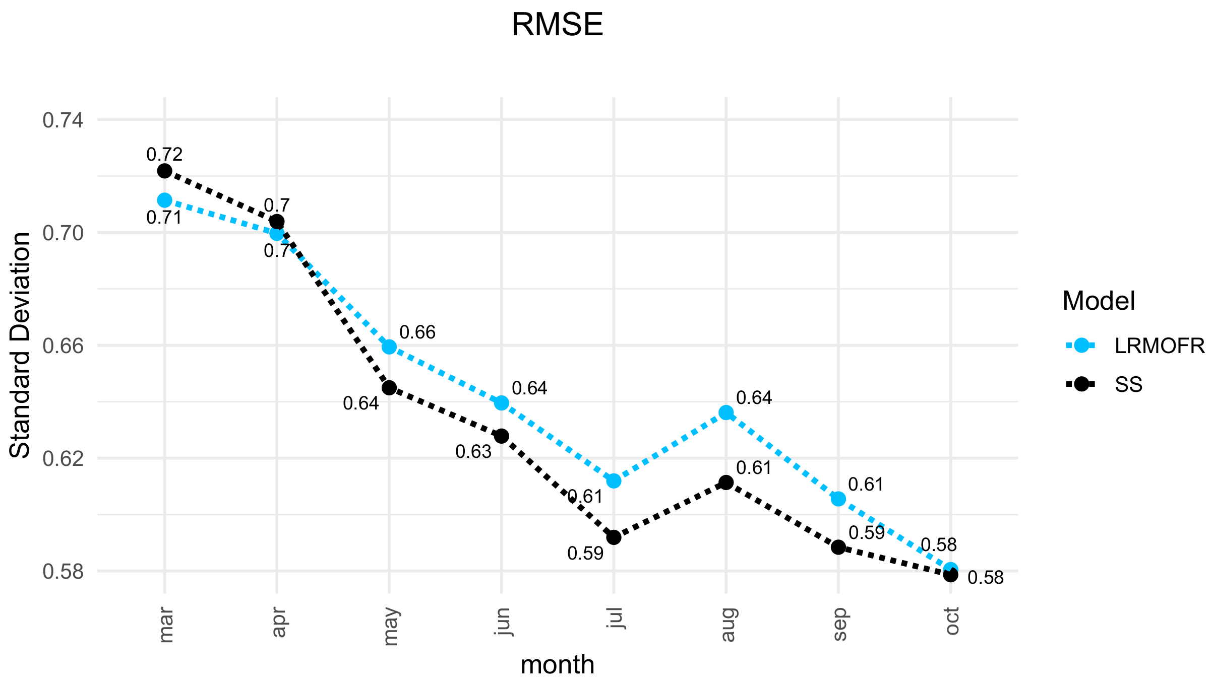
5.1. Prediction Errors of Both Models
We found that in both models, their prediction error generally decreases as the school year progresses (
Figure 1). Coincidentally, the fit between the prediction and the SIMCE results improve as the year progresses (
Figure 2). This trend is expected since the models are receiving the results of the deliberate practice of the students. Every week, students carry out one or two sessions and in each of them, they answer about 24 questions that are part of the formative assessments. However, RMSE does not reach zero. This is partly because the error of the SIMCE test is between 0.26 and 0.35 standard deviations. Therefore, it is not possible for the models to go below that level of error.
It is interesting to observe that in August, both indicators worsen a little bit. Apparently, this is due to the two-week winter break in July. The models receive much less information. In July, students take half of the formative assessments of what they do on the other months.
Figure 1 shows that the RMSE of the state-space model is generally lower than that of the linear regression model, except for the first two and the last month.
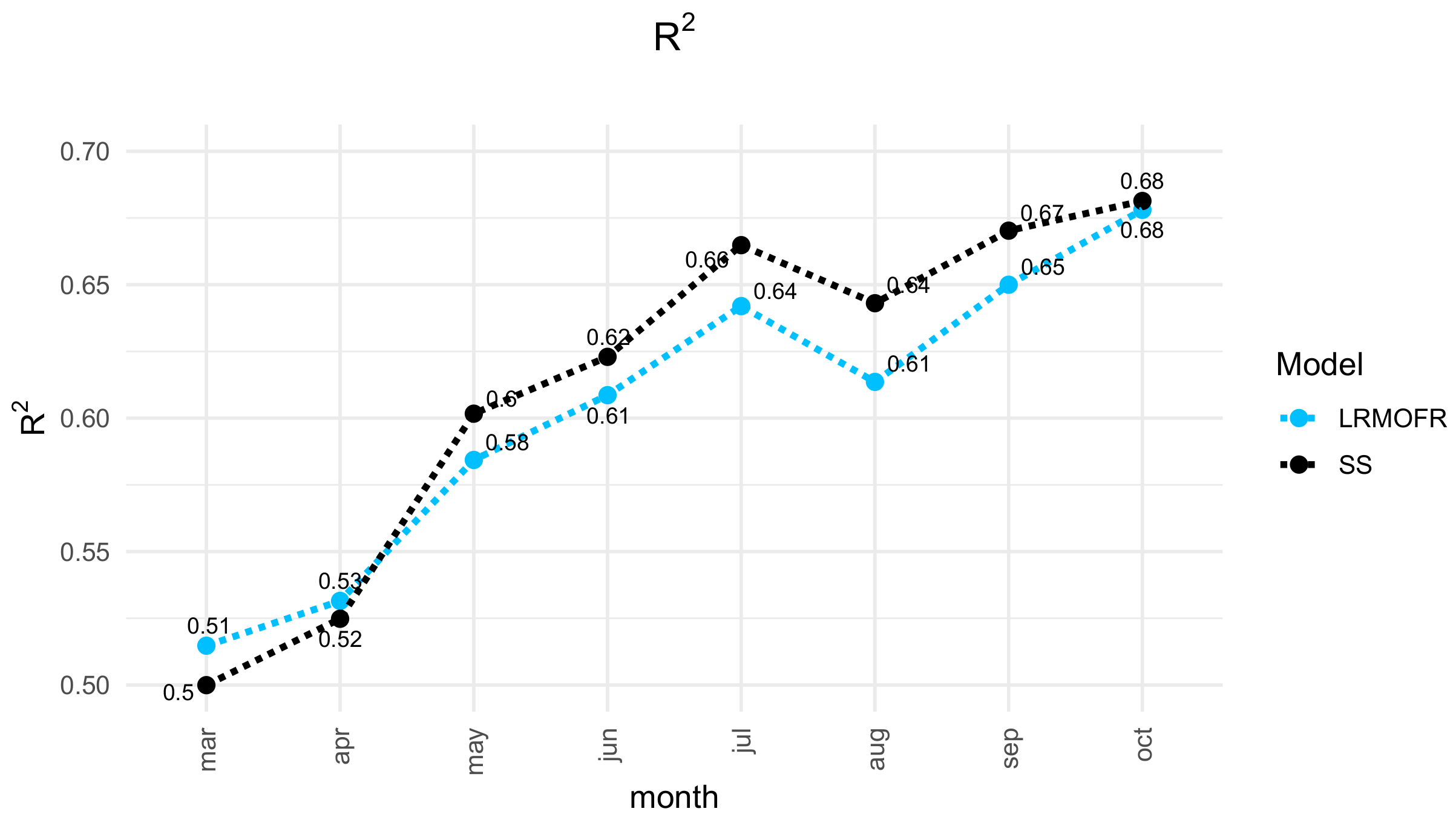
Figure 2 compares R
for the LRMOFR model with R
for the SS model. We see again that in most months, the state-state model has better R
.
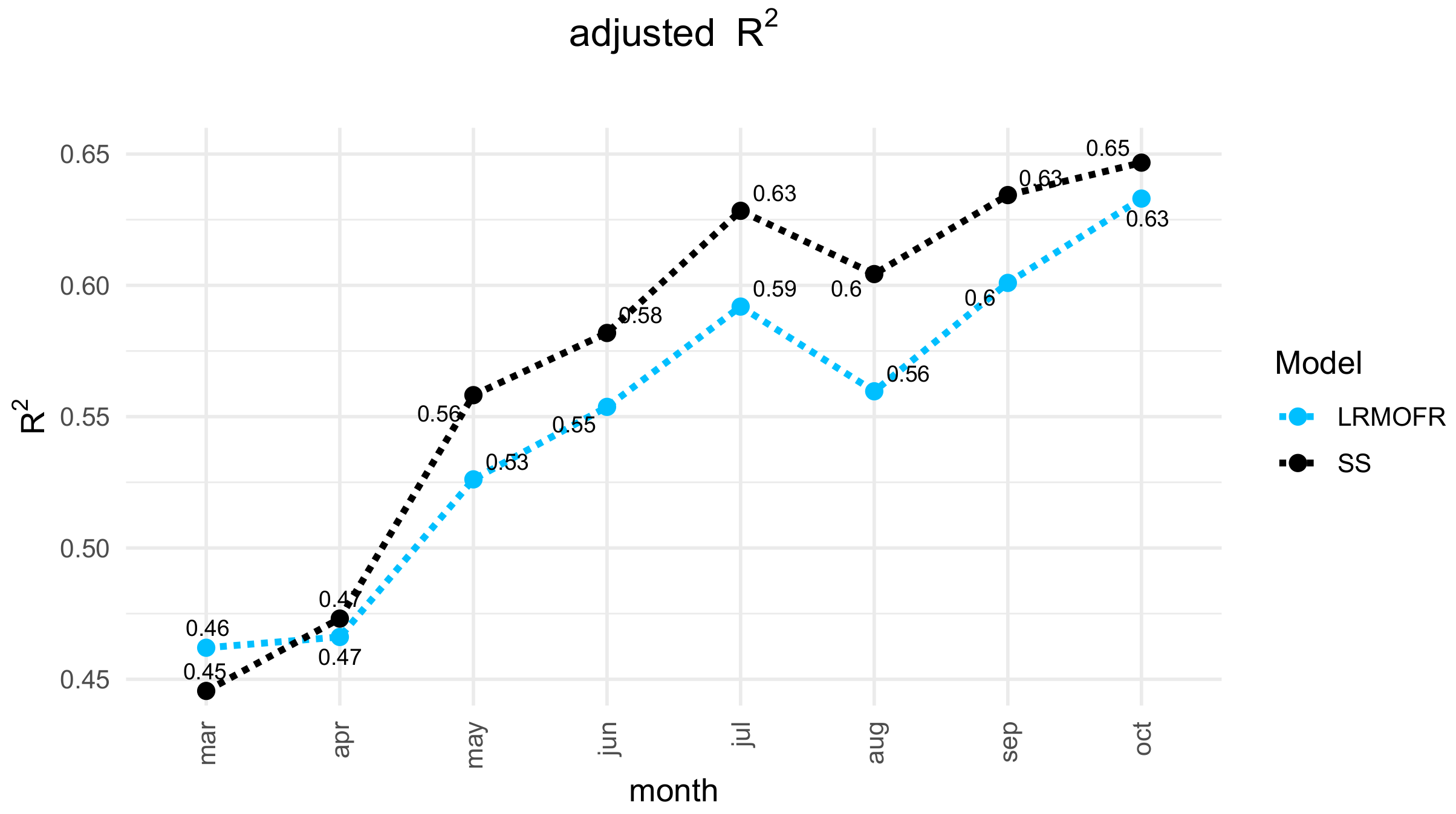
Since the state-space model has much fewer parameters, adjusted R
is even better for the state-space model (
Figure 3).
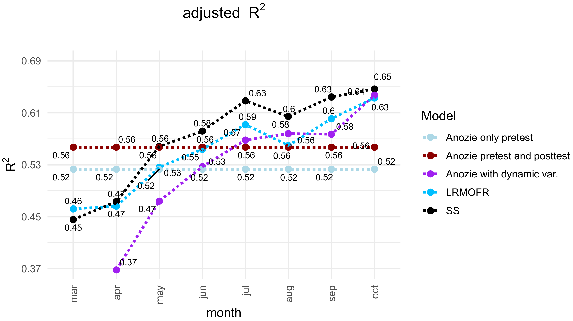
The use of adjusted R
allows comparison with models developed by other authors in other educational systems, for example, with the models of Anozie et al. [
7]. We changed the month in order to be able to compare with those of the Chilean school year. As shown in
Figure 4, the adjusted R
of the state-space model is superior to the other models.
5.2. Optimal Values of the Parameters
For the regression model, we performed 200 cross validations for each month. The results are in
Table 3. The parameters are quite stable.
For the state-space model, we also performed 200 cross validations, but not separated by month. The results are in
Table 4. Again, the parameters are quite stable. We found that
A is basically 1. That is, the state space is a pure accumulator.
A is 1, but K is 0.08. Therefore, is 0.9175. Thus, the predictor uses a forget rate that is close to 8% from one month to the next one. The standard deviation of the random forcing term is low and equal to 0.9 SIMCE points. The standard deviation of the measurement noise is about 10 SIMCE points, which is in the order of that reported by the SIMCE year-end national statistical test.
For the accuracy indicators, the highest parameter B that translates accuracies in SIMCE points is for the data and probabilities strand. However, it does not stand out much from the others. For the other performance indicator, the difference between the number of questions answered correctly on the first attempt and the rest of the questions, the number and operatives strand has a B above the rest of the strands. It is a much larger B than the B’s of the rest of the strands. That is expected, given that the largest number of exercises performed belongs to the numbers and operations strand, and also to the fact that the year-end national standardized test has a lot more questions from that strand. There are some values of B that are negative. This may be because it is perhaps convenient to do fewer exercises of those strands that have less weight in the end-of-year test, and then spend more time practicing exercises of the other strands.
5.3. Contribution of the Different Variables to the Prediction
If we expand the state-space expression, we can compare term by term with the LRMOFR model as shown in
Table 5.
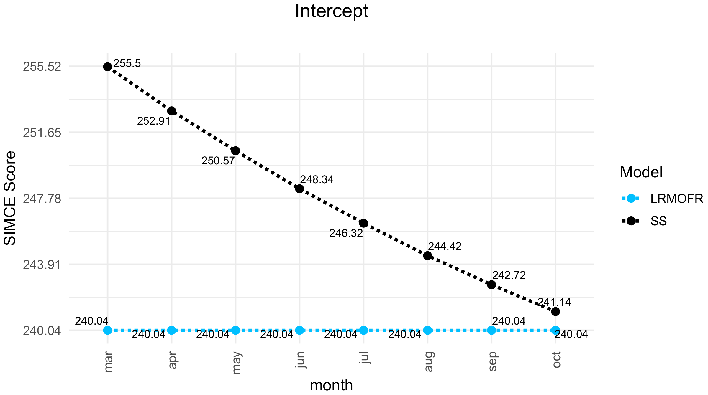
We first analyze the intercept. It is the prediction made each month if we did not have any data on the student. In the case of the LRMOFR model, we impose the same value for all months. In the SS model, there is an initial estimate that falls but is corrected with the observations of each month. The expression for SS is
Since
A is 1, this expression is
We see in
Figure 5 that the values of the intercept of both models are similar and in the last months they coincide.
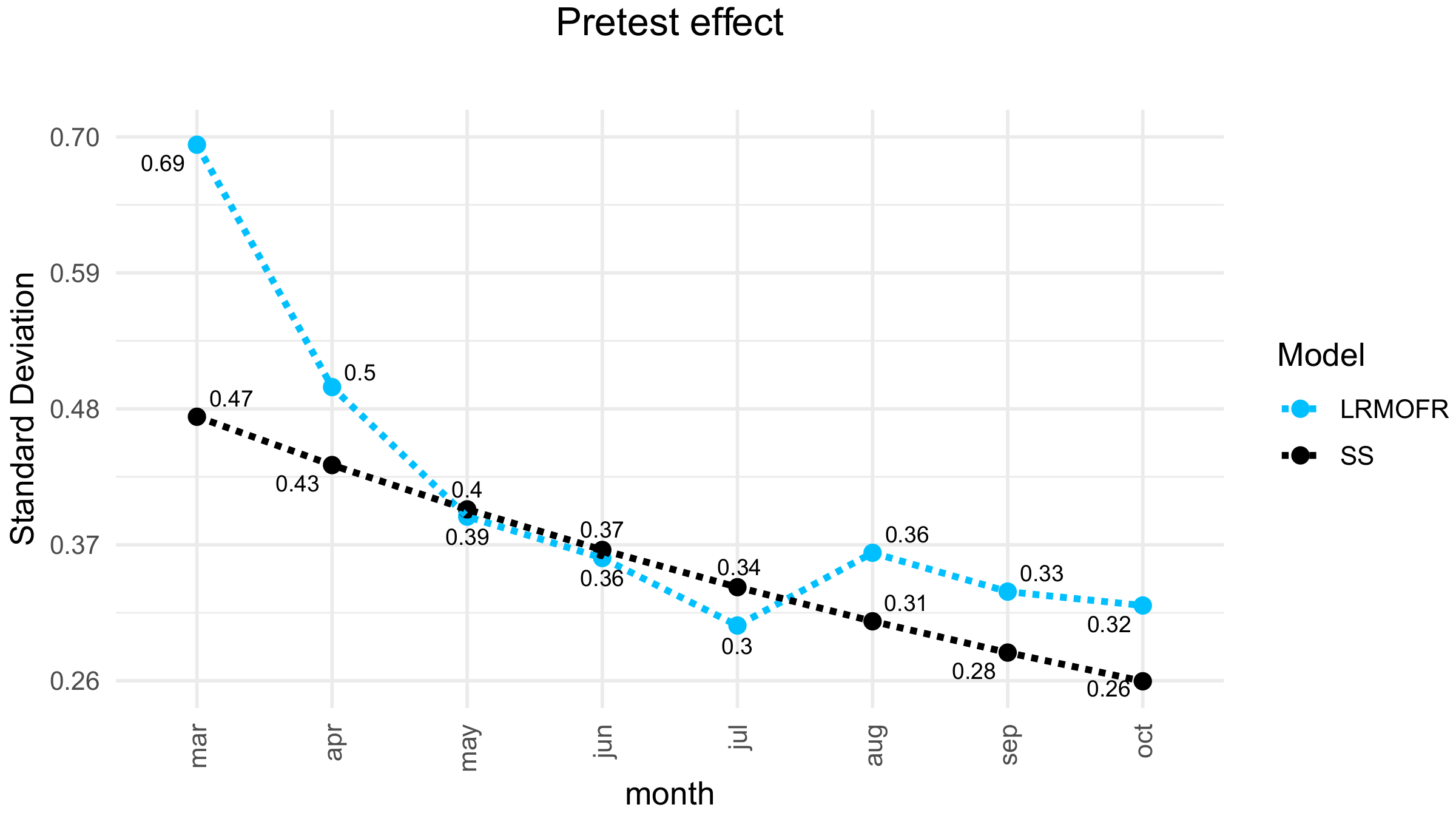
Next, we analyze the effect of the pretest. We increase the pretest on standard deviation and compute its effect on the prediction. In both models, in the first months, the effect of the pretest is much higher than in the later month of the school year (
Figure 6). For the state-space model, the effect is monotonically and exponentially decreasing. In March, one standard deviation increase in the pre-test causes an increase of 0.54 standard deviations in the prediction of the SIMCE score, whereas in October it causes an increase of 0.28 standard deviations. This means that the effect decreases to one half. In the sequence of linear regressions, the effect is also decreasing but rapidly reaches a plateau in May. The graph shows the values of the parameter
presented in
Table 3 and the values of the expression
with the value of the parameters presented in
Table 4 but scaled to standard deviations of the SIMCE test score.
The decay of the effect of the pretest is natural and expected. Given that the platform constantly accumulates the performance of hundreds of exercises performed by the student, then as the times passes by, the pretest information is decreasingly important to predict the result of the end-of-year test. Only at the beginning of the year, the pretest is a highly valuable information. What these models add is the quantification of the decay. In the case of the state-space model, the decay is at a rate of 91.75% from one month to the next. This is a loss of more than 8% per month.
At the classroom level, the greatest effect was one that is a proxy for the classroom climate. It is the average of the responses of all the students in the class to the degree of agreement in a scale from 0 to 5 with the statement that “My behavior is a problem for the teacher”. At the beginning of the school year, in March, an increase of one standard deviation in this response generates a decrease of 0.27 standard deviations in the prediction of the SIMCE score of each student in the course (
Figure 7). By the end of the year, this negative contribution decreases by approximately half. As
Figure 7 shows, the decay of this classroom climate effect in the state-space model is exponential, while in the linear regression model, it is more complex. Moreover, it basically reaches a plateau in June. In the state space, again the decay from one month to the next one of the classroom climate is 91.75%. This is the same as the decay of the pretest. This means that in each variable, the contribution to the end-of-year test drops by 8% from one month to the next.
Figure 7 shows the values of the parameter
presented in
Table 3 and the values of the expression
with the value of the parameters presented in
Table 4, but scaled to standard deviations of the SIMCE test score.
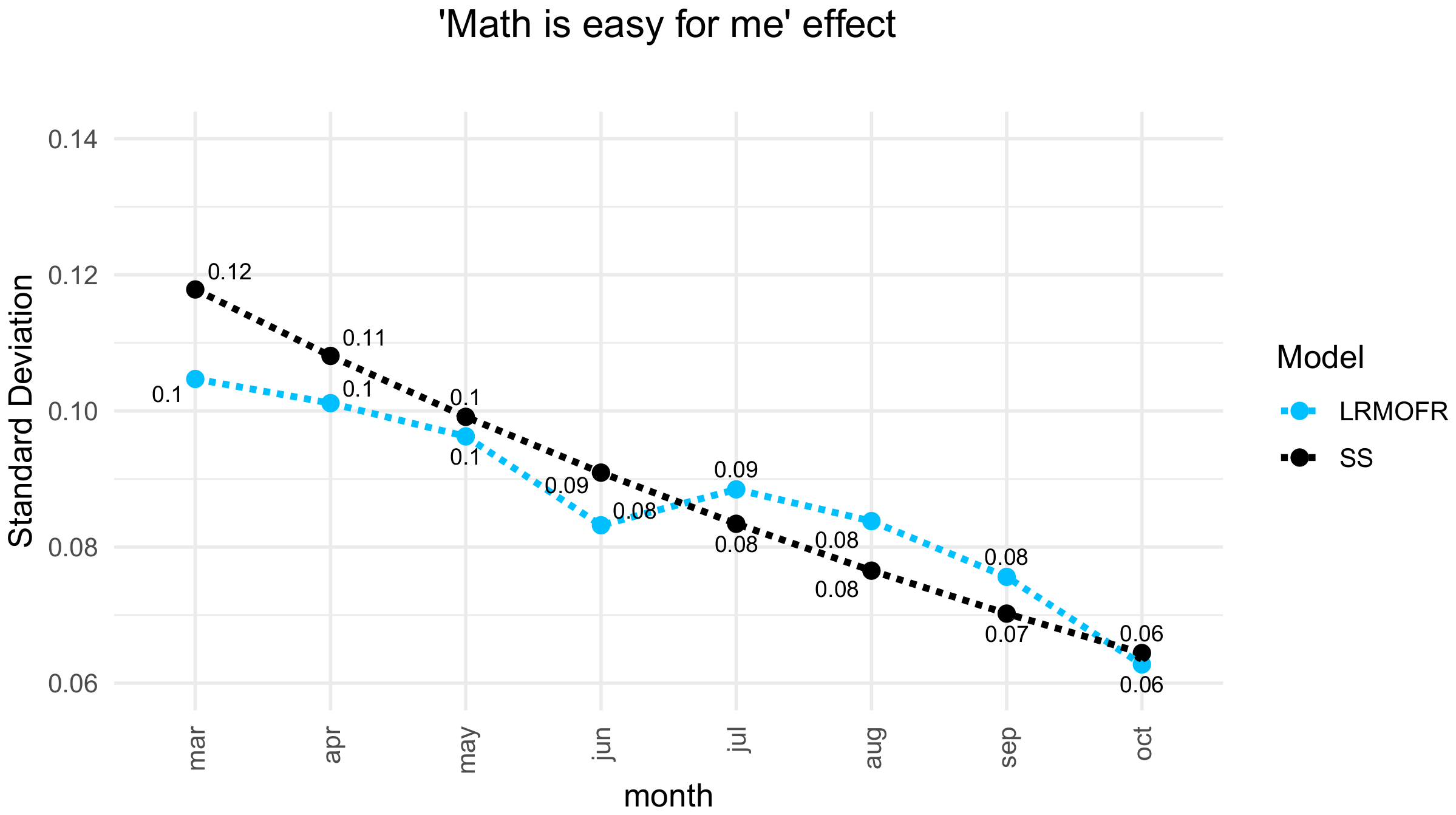
The personal variable that contributes the most to the prediction of the SIMCE score is the belief that mathematics is easy for me (
Figure 8). This is the degree of agreement on a scale of 1 to 5 with “Mathematics is easy for me”. At the beginning of the school year, in March, a student’s one standard deviation increase in that belief causes a 0.12 standard deviation increase in the predicted SIMCE score. However, as the school year progresses, this contribution decreases. At the end of the year, the contribution of this belief reaches half of what it had in March. As
Figure 8 shows, the decay of this effect in the state-space model is exponential, while in the linear regression model, it is more complex. In the state space, the decay of this belief is again a 91.75% from one month to the next, the same as the decay of the pretest and of the class climate.
Figure 8 shows the values of the parameter
presented in
Table 3 and the values of the expression
with the value if the parameters presented in
Table 4 but scaled to standard deviations of the SIMCE test score.
We now compare the effects of the deliberate practice of exercises from each of the five strands of the national curriculum. In each month, we have two performance metrics for the five strands. On the one hand, we have the accuracy. This is the rate of exercises answered correctly on the first attempt. On the other hand, we have the difference between the number of exercises answered correctly on the first attempt and the number of exercises answered correctly on other attempts.
For the LRMOFR model,
Table 3 shows the effects on the prediction of the end-of-year test of a one standard deviation increase in the accuracies. These effects are measured by the parameters
for each curriculum strand and for each month. In general, the effects are positive. The first month of the school year is March. However, this is a month with very little activity since the implementation started in the fourth week of that month. In general, the numbers and operations strand is the one with the greatest effect. Students perform most of the exercises corresponding to this strand. The percentage of exercises that the students performed that belong to this strand is 58.78%. On the other hand, this strand is the one with the most items in the end-of-year SIMCE test. The second strand with the greatest effect is patterns and algebra, which has the greatest effect in July. Then there is the measurement strand, which is the one with the most effect in June. In July and August, the geometry strand has a great effect. Only in October, just before the SIMCE test, does the data and probability strand have the higher effect. This pattern is typical in fourth grade classes in Chile. The data and probability strand is taught at the end of the year.
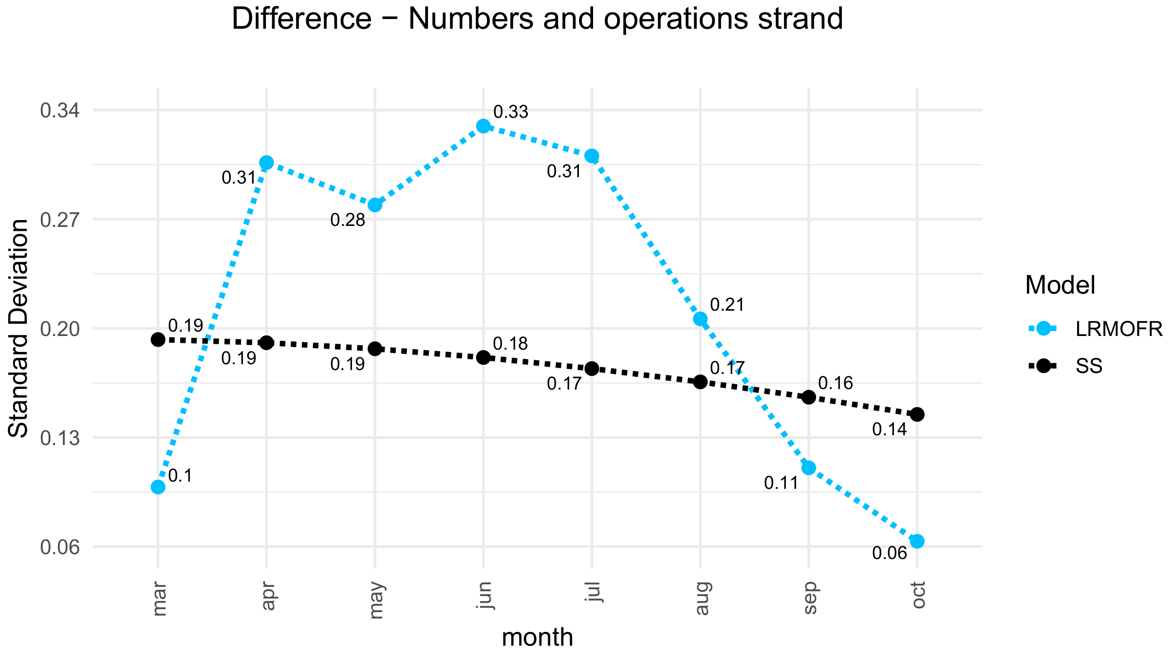
On the other hand, an increase of one standard deviation in the difference between the number of questions answered correctly on the first attempt and the number of questions answered correctly on other attempts generates far more effect on the strand of numbers and operations. This large effect is shown in
Table 3 in the
parameters. The only different month is the final month, October, where the patterns and algebra strand has the highest effect.
Reviewing
Table 4 and comparing the effect values between the LRMOFR and SS models, we see that the effects of the LRMOFR model decay at the rate
. This decay is much faster than the one in the SS model, whose decay rate is
. On the other hand, in the SS model, the effect of the difference in the number of exercises answered correctly on the first attempt and the rest of the exercises is much greater in the numbers and operations strand than in the rest of the strands. However, additionally, that effect is much greater than that of accuracy. Since increasing accuracy can require much more effort, the large effect of this difference suggests that in many cases, it may be worthwhile to increase the number of exercises. For example, if we have an accuracy of 0.7 with 10 exercises, then the difference is 7 − 3 = 4. If we go up to 20 exercises while maintaining the accuracy, then the difference is 14 − 6 = 8. Since B6 is more than three times B1, and since the variables are normalized, then the performance in terms of the difference between questions answered correctly in the first attempt and the number of those not answered correctly in the first attempt has three times the effect of the accuracy. That is, increasing one standard deviation in the difference has three times the effect of raising the accuracy by one standard deviation.
We show in
Figure 9 and
Figure 10 only the case of the numbers strand, which is by far the strand with the highest percentage of exercises performed. The percentage is 65% of the exercises performed in the year.
Figure 9 shows the effect of a student who is one standard deviation above the mean in accuracy each month. In the SS model, we assume that in the future, the student will perform one standard deviation above the mean.
Figure 10 shows the effect of a student who in each month is one standard deviation above the mean in the difference between the number of correct answers in the first attempt and the number of correct answers in another attempt, but assuming that the accuracy is equal to the mean. This means that the student has performed many more exercises, but with accuracy equal to the average of all the students. For example, if the average accuracy is 0.7, then if they performed 7 good exercises on the first attempt and 3 correct exercises on other attempts, there is an accuracy of 0.7 and a difference of 4, whereas if they performed 70 good exercises on the first attempt and 30 correct ones on other attempts, then there is also an accuracy of 0.7 but the difference is 40.
In the SS model, we assume that in the future, the student will continue with a performance of one standard deviation above the mean.
5.4. The Optimal Control Problem: Ask Students to Do Exercises More Carefully or Do More Exercises
In each session, the teacher must decide how many exercises to place and what level of performance will be acceptable. If students make a lot of mistakes, then the teacher may need to stop the practice and explain the core concepts in more detail. The teacher can also assign student monitors to explain and give help to peers as well as asking the students to perform the exercises more carefully and seek help. There may be students responding very quickly and even randomly.
That is, the teacher must decide whether to give more importance to the percentage of correct answers in the first attempt or to the total number of exercises attempted by the students. For example, the teacher has to decide between getting the class to perform 30 exercises per student with 70% of them solved correctly at the first attempt, or to perform only 20 exercises but with 80% them solved correctly at the first attempt. The dilemma is: Which strategy causes better long-term learning? Or, more precisely, which strategy of exercise practicing causes a prediction of a highest score at the end-of-the-year national test?
Consider that we are in the month of
, that is, with complete information on the students up to that month. For the following month
s, the teacher is planning to carry out exercises of strand
k. Therefore, if a student achieves in that month the performance given by
and
, then the predictor of the SS model year-end test result will add the effect
In terms of the accuracy
a, the number of exercises solved correctly at the first attempt
N, and number of exercises solved correctly in other attempts
M, the effect is
with mean and deviation
for
, and
the mean and deviation for
,
.
Rewriting in terms of accuracy and total number of exercises
L, the effect on the predictor of an accuracy
a, and a number of exercises
L to be performed in a month
s after the current month
is given by
Then for a level
, the pairs of accuracies and number of exercises
L for a strand
k with the effect
on month
s posterior to
, the last month with student data, is given by
This expression describes a curve in the
plane.
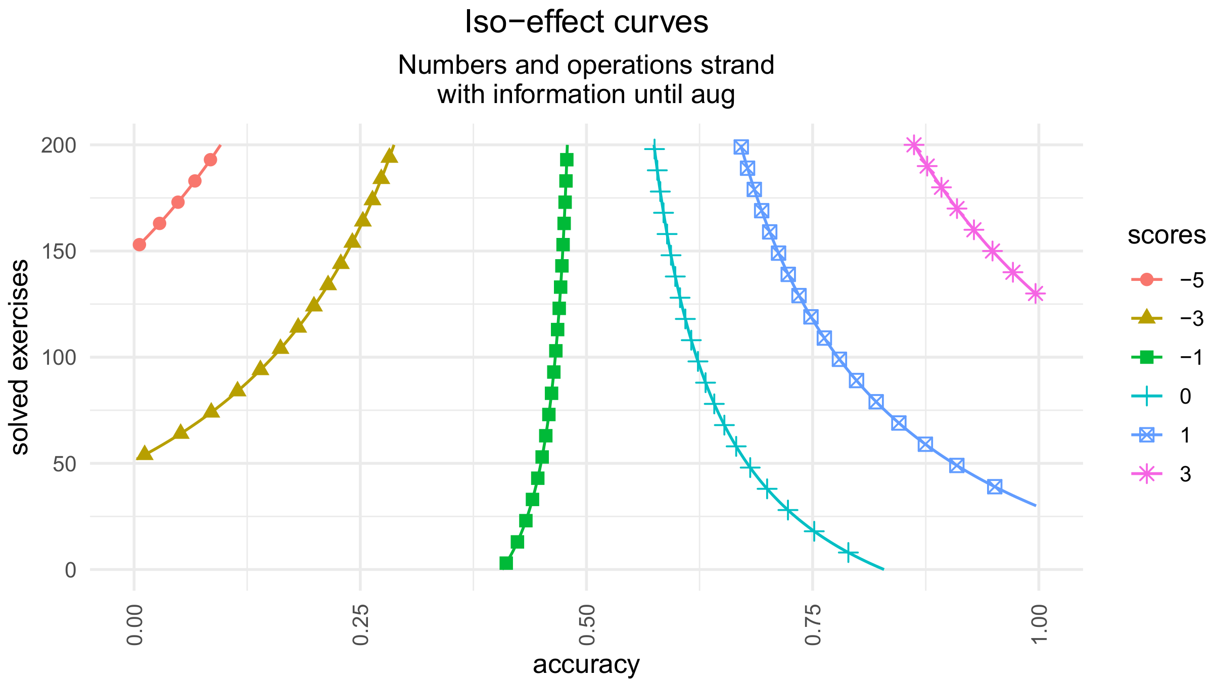
Figure 11 shows the iso-effect curves as a function of the accuracy
a, and the number of exercises
L. Since
A is basically 1, the iso-effect curves do not depend on the month s. However, they do depend on
, through the means and standard deviations of the accuracy and the difference.
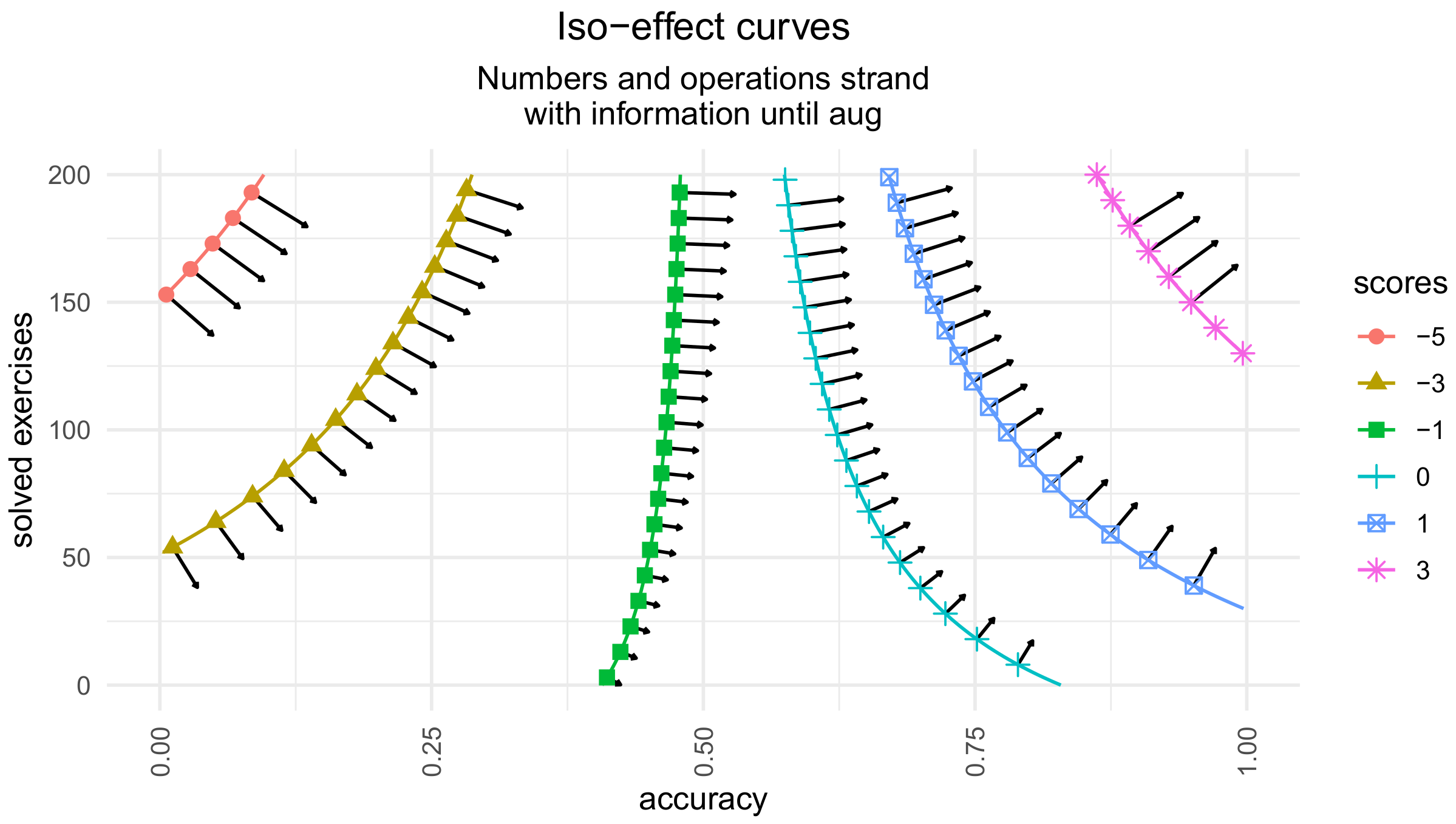
The gradient of the effect with respect to a and
L is
Figure 12 shows the vector field of the gradients superposed to the iso-effect curves for the number and operations strand for the month September when we have information up to August.
From
Figure 12, we see that if the accuracy is below 50%, then it is convenient to reduce the number of exercises to be done but to do them more carefully to improve the accuracy. For example, if we have been doing 130 exercises with an accuracy of 30%, then in order to increase the result of the year-end test, it is better to lower the number of exercises and improve the accuracy. This is due to the fact that in the coordinate (0.30, 130) of the plane
, the gradient points to having higher accuracy
a, but to do fewer exercises,
L.
Let us consider that performing
L exercises with an accuracy
a means an average effort
for the students of the class. It is reasonable, within a range, that by doubling the number of exercises to be performed in a session, the effort doubles. However, the dependence of effort on accuracy is more complex. Let us assume the following dependency:
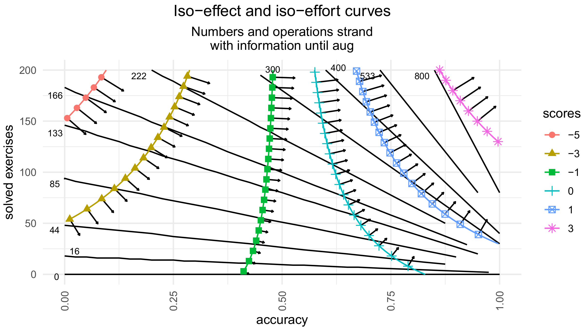
Then, for a given strand of the curriculum, the iso-effort curves are those of
Figure 13. By considering the iso-effect curves or the vector field of gradients, for each strand of the curriculum, for a given level of effort, we can find the optimal combination of accuracy and number of exercises to perform in the session.
In
Figure 13, we can see that for an effort less than or equal to 166, in the numbers and operation strand, the best combination is to plan to perform 40 exercises and with an accuracy of 95%. At that point on the
plane, the effect gradient is perpendicular to the iso-effort curve.
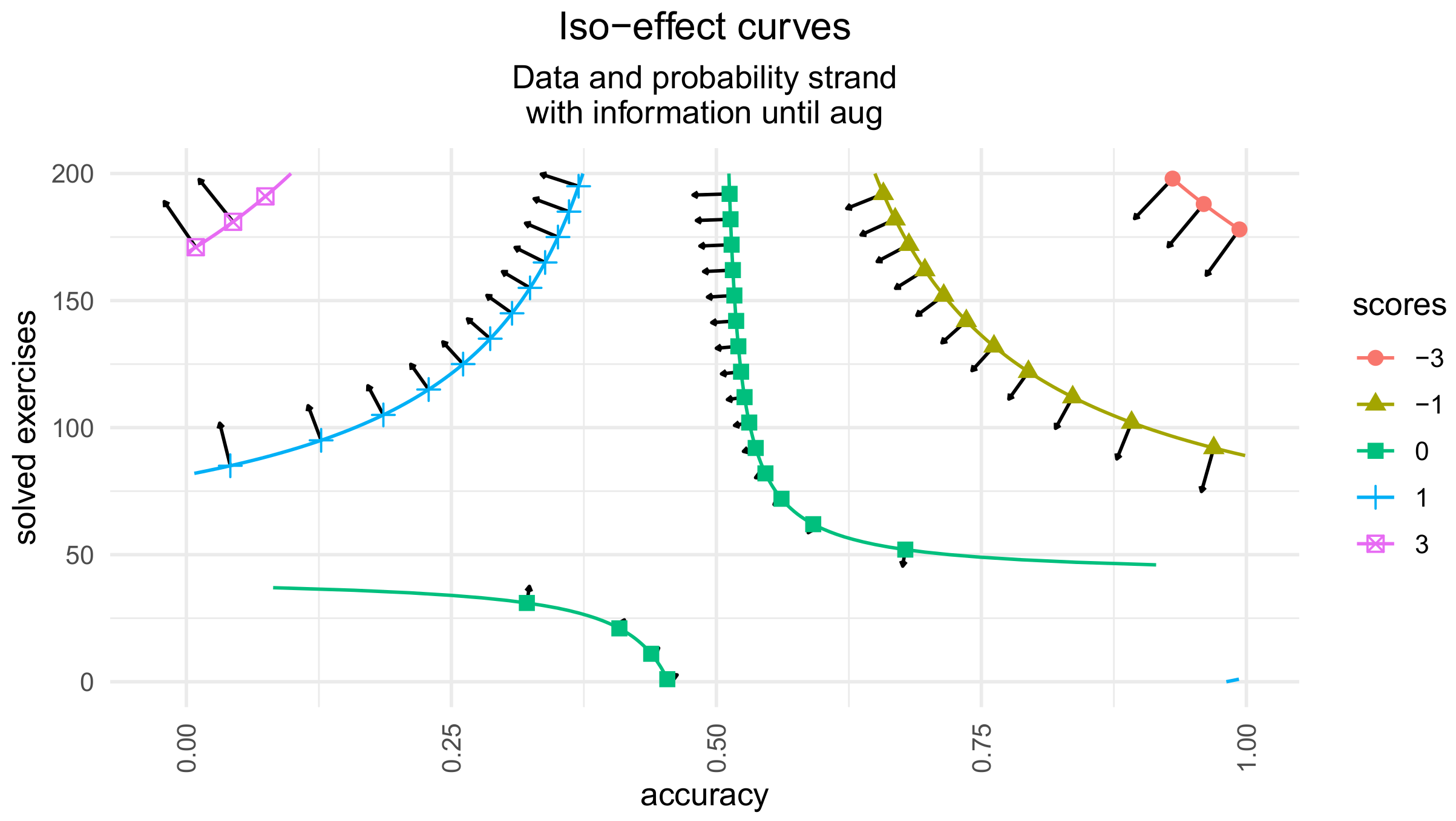
Figure 14 shows that in the data and probability strand, the gradient always points to lower accuracy. One possible explanation is that this may be because it is more effective to spend that effort on other strands.
6. Discussion
Improving the quality of education depends on the quality of transmission of pedagogical practices. Like any cultural phenomenon, improvement depends on access to reliable performance indicators. Good indicators of teaching practices are those that achieve good long-term learning in students. It is therefore necessary for each teacher to be able to estimate and understand the effect of teaching practices on long-term learning. The teacher can then use these estimates to make teaching decisions for every lesson. Therefore, teachers need to be able to predict the effect of applying, in the remaining months, the different options of teaching strategies. In this paper, we consider for each month and curriculum strand two options: how many exercises and with what level of accuracy.
To solve this problem, teachers face several challenges.
First, given that they prefer to pose their own exercises, this generates a large number of questions, each one attempted by a small number of students. Thus, we could not use models based on big data, such as deep learning.
Second, the questions of the national end-of-year tests are unknown to the teachers and there is no public information available on the results of students in each of those questions. For this reason, predicting the results on those tests is much more complex than in other tests. Strategies to predict students’ performance in a question based on the data of the performance of many similar students in similar questions, such as the algorithms used by matrix or tensor factorization or deep learning networks, cannot be directly applied.
Third, another difficulty with predicting long-term learning is that it is not the same as short-term learning. It is not only a phenomenon of decaying and forgetting. It is much more complex. According to [
1], during teaching, what we can observe and measure is performance, which is often an unreliable index of long-term learning. There are strategies that lead to less learning than others in the short term, but generate more learning than the rest over in the long term.
With the information from the responses of 500 students from 24 courses who completed an average of 1089 closed-question exercises on the ConectaIdeas platform during the year 2017, we built two types of models: linear regressions and state-space models. We chose the best option of variables for each of them. We selected those variables analyzing information from 18 courses and we calculated the prediction errors in the remaining 6 courses. We carried out this cross-validation process 200 times. With these results, we can now answer affirmatively the three research questions.
Research Question 1: To what extent can teacher-designed questions (low- or no-stake quizzes) help predict students’ long-term learning as measured by end-of-year standardized state tests?
Despite having questions designed by teachers and each of them answered by few students, the linear regression and state-space models achieve predictions with errors comparable to those of the literature [
7,
29]. We found that with both types of models, we were able to improve the month-to-month predictions. Additionally, the state-space model is in general better than the linear regression model. This better performance is very important because it achieves it with much fewer parameters. The state-space model has only 17 parameters to fit, whereas the linear regression has 106 parameters. That is, the SS model has only 16% of the parameters of the linear regression model. This means that it must be more robust and generalizable to other schools and years.
Research Question 2: To what extent can a hidden Markovian state of the student’s accumulated knowledge up to the current month be estimated so that, along with the probable deliberate practice on the next months, it is sufficient to predict with good accuracy the end-of-year standardized state tests?
The SS model is a simple accumulator that adds monthly performance. From month to month, the predictor adds the score for the new month to the score for previous months. Additionally, the mechanism of the SS model adds the score that it estimates for the following months according to the strategy that the teacher plans to follow. In the first month, the mechanism includes a base score, and the contribution of three sources of information: a pretest, the beliefs of each student, and estimation of the climate of the class. The predictor translates these three contributions into three scores, and adds them. Thus, the teacher has the initial prediction in view and, with the performance of each month, an additive combination to predict long-term learning.
Both models estimate the impact of the pretest and how its impact decreases as the year goes by. This is expected since, as the ConectaIdeas platform accumulates information on student performance, the initial information is less relevant. Likewise, they estimate the impact of students’ beliefs about mathematics. This is very relevant for the teacher, as it gives a clue to determine the importance of this emotional factor and how much effort should be put into dealing with it. Both models also estimate the impact of the class climate on the prediction of each student’s end-of-year test. Again, dimensioning this effect is very relevant for the teacher. It guides to quantify how much effort should be dedicated to improving the climate of the class. In both cases, these effects also decline over the course of the year. In the case of the state-space model, the three effects decay at the same rate. Both models also estimate the effect of the practice of exercises in each of the five strands of the curriculum. The teacher can thus compare the effect of performance on each strand on the prediction of each student’s results on the end-of-year national test. This helps to decide how much intensity to devote to each strand of the curriculum.
A central element of the models is the information for each month. It has two performance elements: the accuracy, which is the percentage of questions answered correctly on the first try; and the difference between the number of questions answered correctly on the first attempt and the rest of the questions. They are very meaningful and very common elements in the daily practice of the teachers. The predictor mechanism just adds those contributions.
A particular characteristic of the SS model is that it includes the effect of strategies on future months. If we use the typical pattern of the student shown in previous months, the predictor uses that pattern and achieves a good prediction in the national end-of-year test. However, the teacher can also try different options for the following month.
Research Question 3: To what extent can a state-space model help teachers to visualize the trade-off between asking students to perform exercises more carefully or perform more exercises, and thus help drive whole classes to achieve long-term learning targets?
The state-space model provides a very transparent and simple prediction mechanism. First, it has very few parameters. They are just what is needed. As there are 5 strands in the Chilean mathematics curriculum, and in each one we have 2 performance metrics, this already brings together 10 parameters. They are parameters that translate both performances in the five strands into the corresponding contribution to the test score. The rest are that the parameters translate into the test score the contribution of the pretest, the beliefs about ease in mathematics, and the climate of the class. Finally, there is the rate of forgetting from one month to another.
Second, the whole mechanism is an additive one. The score of each contribution is added with the rest.
Third, the peculiarity of the state space model is that from one month to another, the mechanism updates the prediction in a Markovian way. It is enough to have the predictor of the last month, not the whole history of information. This is a huge advantage, as last month’s predictor sums it all up. It is not necessary to go to gather information from previous months.
Fourth, for each month and for each strand, the mechanism is a tool that helps the teacher to see the effect of her decisions. She can visualize ahead the effect of choosing how many exercises to request and what minimal accuracy to request. In a 2D graph, the teacher can see the iso-impact curves of these two decisions.
Fifth, the teacher can also visualize the arrows of the gradients. They are an intuitive visualization that indicates how to move to achieve more impact in the national test at the end-of-the-year. This allows the teacher to design her optimal strategy for driving the entire class toward the goal of greatest long-term learning. It is not a black box recommending what to do. It is a tool that allows the teacher to simulate and visualize the effect of different strategies.
Sixth, the teacher can also superimpose the iso-effort curves in order to find an optimal solution. That is, she can seek the combination of the number of exercises and accuracy in order to achieve the greatest long-term learning while maintaining a limited and predefined level of effort. That is, not only the state-space model gives the teacher an understanding of the factors involved and how they contribute to the result of the end-of-year summative test. It also gives her a tool to simulate the effect of various practice strategies. It is a very natural and intuitive way to visualize the trade-off between asking students to perform exercises more carefully or perform more exercises. In summary, in this paper, we built a state-space model with control variables that allow the teacher to visualize an optimal control strategy in order to conduct sessions that achieve the best long-term learning.
Although there are applications of optimal control to student learning strategies [
30,
31,
32,
33], these are problems formulated with abstract situations. They do not include empirical data on classes with students, models that fit those data, and end-of-year national standardized tests that independently measure long-term learning. To the best of our knowledge, this is the first time that the problem faced by each teacher is presented as an optimal control problem, with whole year empirical data of hundreds of students in several classrooms, and where a very practical solution is proposed. Moreover, we developed a graphical tool, intuitive and easily understandable, that helps teachers visualize the effect of strategies. With this state-space formulation and with the iso-impact and iso-effort curves, at each session, the teacher can review what students have achieved in previous sessions, and decide how to drive the entire class from then on.
There are several aspects to investigate and develop in the future. One is to include an interaction between strands of the curriculum. In a previous study, we empirically identified the effect of some topics on others [
16]. We plan to include this interaction in the state-space model. Another aspect is to incorporate the effect of written answers to open questions [
21,
25]. We already did this for a linear regression model. We plan to include this information in the state-space model. There is also the effect of different strategies that the teacher can choose for deliberate practice. For example, the effect of spacing and interleaving [
34,
35]. Spacing is not doing all the exercises at once. For example, 6 h of deliberate practice in a type of exercise is not the same as doing it in spaces of 1 h for six different days. On the other hand, in interleaving, in each session, students solve a random mixture of different types of problems. Interleaving and spacing are cases of variability in practice. Experimental evidence has shown that variability generates more long-term learning and generalization, and in various domains and tasks [
36]. Another important topic is to include the effect of conducting peer reviews of the written response to open-ended questions. Finally, there is the effect of peer tutors [
24]. We plan to include these strategies in future state-space models.
7. Conclusions
This work connects with previous literature in several respects. On the one hand, it implements in several schools the strategy of systematic deliberate practice. This strategy has been studied mainly in research laboratories for the study of human cognition and learning [
1,
2,
3]. Instead, in this paper, we study the typical situations found in schools. It is a situation where instructors choose or create their own questions to adjust better to the realities of their classes. Furthermore, we adhere to the tight restrictions of low SES schools. On the other hand, in this paper, we connect with the long-term learning prediction literature [
7,
8,
9]. Moreover, we connect with the month-by-month predictions proposed by [
7]. However, we do so with a state-space model that has the advantage of few parameters and greater interpretability. Additionally, we connect with the literature on optimal control in learning [
30,
31,
32,
33], but we do it contextualizing in elementary education and with empirical data from hundreds of students who answered a large number of questions during the year. We also do it by proposing a graph that gives the teacher a direct visualization of the impact of two basic strategies: for each strand of the curriculum, how many more exercises to include and what percentage of correct answers students should try to achieve in the following month.
7.1. Theoretical Implications
In the theoretical framework of the evolutionary educational psychology, the challenge of teaching school mathematics is due to an evolutionary mismatch or evolutionary trap [
12]. The evolved cognitive systems and inferential biases that define the natural knowledge required for hunting–gathering life are not sufficient for academic learning [
37]. Our brain is not adapted to learning these types of radically new concepts. It does not cost us very much to learn to walk or speak. We do it even without a teacher. However, learning to read and write provokes a huge change that greatly affects different brain areas [
38]. Similarly, learning the mathematical concepts of the curriculum requires a lot of effort and deliberate and constant practice, day by day, for many years.
However, implementing a deliberate practice strategy is not easy. There are several challenges. On the one hand, the teacher has a huge motivational problem to solve. It is easy to say that you have to make students practice, but actually making all students do it systematically is not that simple. The teacher has to deal with the motivation and beliefs of each student, as well as with the climate of the entire class. The teacher must also take into account the prior knowledge of each student and the progress they are making. The teacher must continually decide between how much to exercise, what level of difficulty and what percentage of correct answers to achieve. There is a curriculum to cover and a national end-of-year test target. All students must perform well. This is an optimal control problem, where the teacher must guide dozens of autonomous agents, each one with their own strengths and motivations. The teacher has to lead a complex swarm of agents in order to reach a predefined target. Every student must achieve the optimal long-term learning, given their initial condition and the condition of the class.
To reach this goal, the teacher needs to be able to predict the effect of deliberate practice on the long-term learning of each student. However, the teacher also needs to have a simple-to-understand tool that allows to simulate deliberate practice alternatives for the next month and know the impact they will have on long-term learning.
In summary, we found that this type of system is feasible to implement. With the ConectaIdeas platform, students carry out intensive deliberate practices that allow the teacher to predict their long-term learning each month. In addition, the platform can provide the teacher with tools to guide on how to conduct the practice of the whole class in the next month.
7.2. Managerial Implications
The results found in this paper give some ideas to introduce management components in online platforms that support the teacher to lead the whole class to the learning target. We learned three practical ideas.
First, it is possible to build a module that each month tells the teacher the prediction of long-term learning for each student. We found that the prediction error is reasonable and decreases month by month.
Second, the module can indicate the weight of socio-emotional factors, such as students’ beliefs about mathematics. It can also include the effect that the climate of the class can have for the prediction of the long-term learning of each student. This will allow the teacher to take personalized strategies to handle socio-affective states of each student. It also supports the teacher to design strategies directed to improve the learning environment of the whole class. The teacher will know how important these factors are for her course and then decide on a plan of action. She will be able to compare the effect of these variables with respect to others, such as initial performance and the effect of practice.
Third, the module can help the teacher visualize how to plan a deliberate practice schedule for the coming month. It will help her to determine, for each student and each strand of the curriculum, the effect of planning a given number of exercises and trying to achieve a percentage of correct answers. These are basic indicators for action in the following month.


