Applications of Markov Decision Process Model and Deep Learning in Quantitative Portfolio Management during the COVID-19 Pandemic

Abstract

Whether for institutional investors or individual investors, there is an urgent need to explore autonomous models that can adapt to the non-stationary, low-signal-to-noise markets. This research aims to explore the two unique challenges in quantitative portfolio management: (1) the difficulty of representation and (2) the complexity of environments. In this research, we suggest a Markov decision process model-based deep reinforcement learning model including deep learning methods to perform strategy optimization, called SwanTrader. To achieve better decisions of the portfolio-management process from two different perspectives, i.e., the temporal patterns analysis and robustness information capture based on market observations, we suggest an optimal deep learning network in our model that incorporates a stacked sparse denoising autoencoder (SSDAE) and a long–short-term-memory-based autoencoder (LSTM-AE). The findings in times of COVID-19 show that the suggested model using two deep learning models gives better results with an alluring performance profile in comparison with four standard machine learning models and two state-of-the-art reinforcement learning models in terms of Sharpe ratio, Calmar ratio, and beta and alpha values. Furthermore, we analyzed which deep learning models and reward functions were most effective in optimizing the agent’s management decisions. The results of our suggested model for investors can assist in reducing the risk of investment loss as well as help them to make sound decisions.

1. Introduction

Quantitative portfolio management (QPM) is a basic financial task to obtain optimal returns while avoiding risk at the same time. In recent years, due to the improvement of computational power and the increase of research on sequential decision making through Markov decision process (MDP), deep reinforcement learning (DRL) has achieved great success in many fields (such as self-driving technology [1], game playing [2,3], and resource optimization [4]), and more and more people are beginning to apply it in the field of quantitative management [5]. In essence, QPM involves continuous decision making of buying or selling assets according to the latest market information to achieve the management goal. The intrinsic advantage of reinforcement learning (RL) is that it can directly learn action strategies in the process of interacting with the dynamic financial environment and [6,7] has achieved promising results in QPM.

The financial market is highly volatile and non-stationary, which is totally different from game or robot control. A stable profit strategy is still the common pursuit of researchers. Yang et al. [8] employed three actor–critic-based algorithms and proposed an ensemble strategy that automatically selects the best-performing agent to trade based on the Sharpe ratio, allowing the trained agent to adapt to various market conditions. Chen and Huang [9] proposed a multimodal learning model that incorporates an influence model for assessing the impact of news on the market. The results of the experiment demonstrated that the influence model improved the ability of RL agents to generate profits. Liu et al. [10] utilized imitation learning techniques to balance the exploration and exploitation of the RL agent, and comparison results confirmed its ability to generalize to various financial markets.

However, the above studies ignore the augmentation of the original input features because the original price data and technical indicators are not suitable to be directly put into the state space. First, the high instability, low signal-to-noise ratio, and external shock characteristics of the real financial market mean that the input of the original financial features in the state space may bring serious problems to the estimation of the value function [11]. Second, putting the OHCLV (open, high, close, low, volume) data and a tremendous number of technical indicators into state space would result in the curse of dimensionality [12]. Many existing studies have simplified the state space as OHCLV data and a few technical indicators [13,14,15,16]. A better solution is to extract the latent feature through the feature augmentation model, which can reduce the calculation cost and time required for training and eliminate redundant information between related features [17].

To the best of our knowledge, there are few studies devoted to augmenting the quality of features before implementing the trading algorithms. Yashaswi [18] proposed a latent feature state space (LFSS) module for filtering and feature extraction of financial data. LFSS includes the use of the Kalman filter and a variety of machine-learning-based feature-extraction technologies to preprocess the feature space, including ZoomSVD [19], cRBM [20], and autoencoder (AE) [21]. Among them, the AE has the best effect and is superior to the preprocessed RL agent and five traditional trading strategies. Soleymani and Paquet [22] employed a restricted stacked autoencoder module in order to obtain non-correlated and highly informative features and the results demonstrated the efficiency of the proposed module. Li [23] proposed a feature preprocessing module consisting of principal component analysis (PCA) and discrete wavelet transform (DWT), and the numerical results demonstrate that feature preprocessing is essential for the RL trading algorithm.

Moreover, the high instability of the financial market will also make it difficult to define an appropriate reward function. The change rate of portfolio value is commonly defined as reward function. However, it represents less risk-related information than risk-adjusted technical indicators such as Sharpe ratio, Sortino ratio, and Calmar ratio. Thus, many studies [10,24,25,26] using Sharpe ratio [27] as the reward function and their back-test performance improved significantly in terms of maximum drawdown (MDD). Wu et al. [28] introduced the Sortino ratio as the reward, which only factors in the negative deviation of a trading strategy’s returns from the mean, and Almahdi & Yang [29] introduced the Calmar ratio based on MDD, all achieving better performance. However, the technical indicators we mentioned above only use the first two statistical moments of yield distribution, namely mean and variance, which does not take into account the high apex and thickness tail property and bias characteristics of the real return series [30]. In addition, MDD measures the maximum loss over a long period of time, which does not reflect the risk in the short period [31]. It is particularly vulnerable to extreme events, which can result in significant losses yet occur infrequently, so they are hardly probable. To address the defects of the above risk adjusted indicators, we introduced the omega ratio to construct a novel reward function to better balance the risk and profit. Compared with the three indicators mentioned above, the omega ratio is considered to be a better performance indicator because it depends on the distribution of all returns and therefore contains all information about risks and returns [32]. From the perspective of probability and statistics, it is a natural and enlightening in financial interpretation.

In this paper, to address the aforementioned challenges and issues, we propose a Markov decision process model-based deep reinforcement learning model for QPM, called SwanTrader. The proposed model consists of two main components: a multi-level state space augmentation (MSA) and a RL agent trained by an on-policy actor–critic algorithm. The MSA comprises a stacked sparse denoising autoencoder (SSDAE) network and a long–short-term-memory-based autoencoder (LSTM-AE) network. SSDAE is performed on the financial data to extract the robust features, and then, the timing-related information is further extracted by LSTM-AE. The RL agent is implemented by the advantage actor–critic algorithm (A2C) with augmented state features, action, and a novel risk-adjusted reward. To evaluate the performance of SwanTrader, we conduct experiments on a real-world dataset containing the COVID-19 period to extend the literature related to financial behavior of individual investors during the COVID-19 pandemic [33,34,35,36]. The results show that the management policy optimized by the proposed model strikes a good balance between risk and return. SwanTrader outperforms the traditional trading strategies (such as EW, CRP, EG, Anticor, CORN, and ONS), the state-of-the-art model [8], and other DRL-based state space augmentation models [23] in terms of accumulative return, Sharpe ratio, MDD, and alpha and beta. Specifically, our main contributions are summarized as follows:

• We suggest a RL model for quantitative portfolio management and propose a multi-level deep learning network that takes into account the instability and temporal correlation of the market.
• We extend the A2C to the stock market, and the experiments show that the proposed model is robust and practical during the COVID-19 pandemic with seven baselines.
• We introduce the omega ratio as our real-time reward function to address the defects in the Sharpe ratio, Sortino ratio, and MDD.

2. Related Works

2.1. Reinforcement Learning Algorithms

In the realm of quantitative management, the application of DRL has proliferated in recent years. There are three forms of algorithm usage: the value-based model, the policy-based model, and the actor–critic model [37].

The value-based approach, which is the most prevalent way and aids in solving discrete action space problems with techniques such as deep Q-learning (DQN) and its enhancements, trains an agent on a single stock or asset [38,39,40]. Due to the consistency of price data, it would be impractical to apply this model to the task of investing in a large quantitative management task. The policy-based approach has been implemented in [6,41,42]. Policy-based models, as opposed to value-based models, which may be the optimal policy for some issues, are capable of handling the continuous action space, but it will result in a high square difference and a sluggish learning speed [42].

The actor–critic model attempts to combine the benefits of the value-based and policy-based approaches. The objective is to simultaneously update the actor network representing policy and the critic network representing value function. The critic estimates the value function, and the actor uses the strategy gradient to update the critic-guided strategy probability distribution. The actor network learns to take better actions over time, while the critic network becomes more adept at evaluating these actions. Due to its outstanding performance, the actor–critic model has garnered considerable attention. Reference [43] compared the representative algorithms of the three mentioned models: PG, DQN, and A2C. The results present that the actor–critic model is better than the value-based and policy-based models, showing more stability and stronger profitability. Reference [28] showed that the actor–critic model is more stable than the value-based in the ever-evolving stock market. Reference [44] employed three actor–critic algorithms, including the proximal policy optimization (PPO), the deep deterministic policy gradient (DDPG), the advantage actor critic (A2C), and the twin delayed DDPG (TD3), and tested them on the Indian stock market. On comparing the results, the A2C indicates the best results. Reference [45] employed DDPG, PPO, and A2C in portfolio-management tasks, and the result indicates the PPO is slightly higher than the A2C in terms of the Sharpe ratio. Reference [8] conducted a comparison of PPO, A2C, and DDPG. Experimental results indicate that A2C outperforms other algorithms. In summary, this paper employed A2C and implemented it using stable-baselines3 [46].

2.2. Feature-Augmentation Model

Feature-augmentation models have been extensively studied in many fields. Reference [47] proposed a defense solution based on a deep denoising sparse autoencoder (DDSA) to improve the robustness of DNNs against adversarial attacks. The results on the MNIST and CIFAR-10 datasets indicate that DDSA defense is highly robust and outperforms state-of-the-art defense models. Reference [48] presented a stacked autoencoders (SAEs) network to generate deep high-level features for predicting the stock price. The results show that the proposed model outperforms other similar models in predictive accuracy. Reference [49] utilized an autoencoder-LSTM model to predict the volatility of FX, outperforming the traditional LSTM model.

Based on the above-mentioned study, we present the multi-level state space augmentation (MSA) for RL in quantitative trading. The MSA comprises a stacked sparse denoising autoencoder (SSDAE) network and a long–short-term-memory-based autoencoder (LSTM-AE) network. The SSDAE is performed on the financial data to extract the robust and informative features, and then, the timing-related information is further extracted by the LSTM-AE. Specifically, the reasons why we use LSTM-AE for higher level extraction are as follows: (1) considering that RL agents only rely on the latest state information to make decisions, the LSTM network can save the state information before inputting the network so that the extracted latent features contain historical information and (2) time series correlation of financial data. We utilize the LSTM module to capture the temporal patterns based on market observations.

3. Preliminary and Background

3.1. Markov Decision Process (MDP) Model

Our portfolio-management model assumes that the agent would invest in a portfolio over a period of time. As is customary, we keep a portfolio of m+1 assets, with one risk-free asset (balance b) and m risky stock assets, which can be modeled by the Markov decision process (MDP), and our goal is expressed as the maximization of total reward. MDP is defined as the tuple ($\mathcal{S},$$\mathcal{A},\mathcal{P},$$r$$,\gamma$: $\mathcal{S}={{\displaystyle \cup }}_t{\mathcal{S}}_t$ is a vector in which the information represents the environment information perceived by the agent. $\mathcal{A}={{\displaystyle \cup }}_t{\mathcal{A}}_t$ is a vector of actions over all assets. The allowed actions on each stock include selling, buying, or holding, which result in decreasing, increasing, or no change of the stock shares h, respectively. $\mathcal{P}$: $p\left(s_{t+1}\mid s_t,a_t\right)$ represents the probability of selecting action $a_t\in \mathcal{A}$ from $s_t\in \mathcal{S}$ to the next state $s_{t+1}\in \mathcal{S}$, and $r$ is the direct reward of taking action at state $s_t$ and arriving at the new state $s_{t+1}$, which indicates how well the agent is doing at a discrete time step t. γ ∈ (0, 1] is the discount factor. The policy $\pi$ is a mapping that specifies the action to take in a specific state, and the agent’s objective is to maximize its expected return to find an optimal policy ${\pi }^{\ast }$ given the initial distribution:

$${\pi }^{\ast }=\underset{\pi }{\arg max}{\displaystyle \sum }_{t=0}^T{\mathrm{E}}_{\left(s_t,a_t\right)\sim {\rho }_{\pi }}\left[{\gamma }^{t}r\left(s_t,a_t\right)\right]$$

(1)

where ${\rho }_{\pi }$ indicates the distribution of state-action pairs that RL agent will encounter under the control of policy $\pi$.

For each policy $\pi$, one can define its corresponding value function:

$$V_{\pi }\left(s_t\right)={\mathrm{E}}_{a_t\sim \pi }\left[Q_{\pi }\left(s_t,a_t\right)\right]$$

(2)

The management environment of this paper follows Yang et al. [8]. The state space of our trading environment consists of four components [$b_t,h_t,p_t,X_t$]. Here are the definitions for each letter:

• $b_t$ ∈ ${ℝ}_{+}^{}$:available balance at current time-step t;
• $h_t$∈ ${\mathbb{Z}}_{+}^n$: shares owned of each stock at current time-step t;
• $p_t$ ∈ ${ℝ}_{}^n$: close price of each stock at current time-step t;
• $X_t$ ∈ ${ℝ}_{}^n$: augmented features at current time-step t.

In the quantitative management task, it is the agent’s job to decide the buy and sell quantities of each stock in the portfolio. For a single stock, our action space is specified as {−k, −1, 0, 1, …, k}, where k and −k indicate the number of shares that can be purchased and sold, respectively, and $\mathrm{k}\le {\mathrm{k}}_{\max }$. ${\mathrm{k}}_{\max }$ is a predefined parameter that specifies the maximum number of shares for each buy/sell action. The action vector will be normalized to [−1,1], indicating that it is continuous.

3.2. Assumption and Constraints

In order to mimic the real market management process in this research, we conformed to the following widely held assumptions [7,22,50,51]: If the volume of traded assets on a market is high enough, adequate liquidity, minimal slippage, and no market influence are all attainable.

• Adequate liquidity: All market assets are liquid, allowing for the same conditions to be applied to every transaction.
• Minimal slippage: As a result of the high liquidity of the assets under consideration, orders can be executed swiftly at the close price with minimal or no loss in value.
• No market influence: The agent’s trading volume is so negligible relative to the size of the entire market that the agent’s transactions have no effect on the state transition of the market environment.

Additionally, we identify the following limits that represent our concerns regarding practice:

• In our action space, we prohibit shorting assets; we do not permit investors to borrow assets and return them in the future; and we do not permit investors to borrow assets and return them in the future.
• The transaction cost is a constant proportion of daily trade volume.
• Nonnegative balance b ≥ 0: Permitted acts should not result in a negative balance. The stocks are separated into sets for buy and sell action based on the activity at time t.

4. Data and Methodology

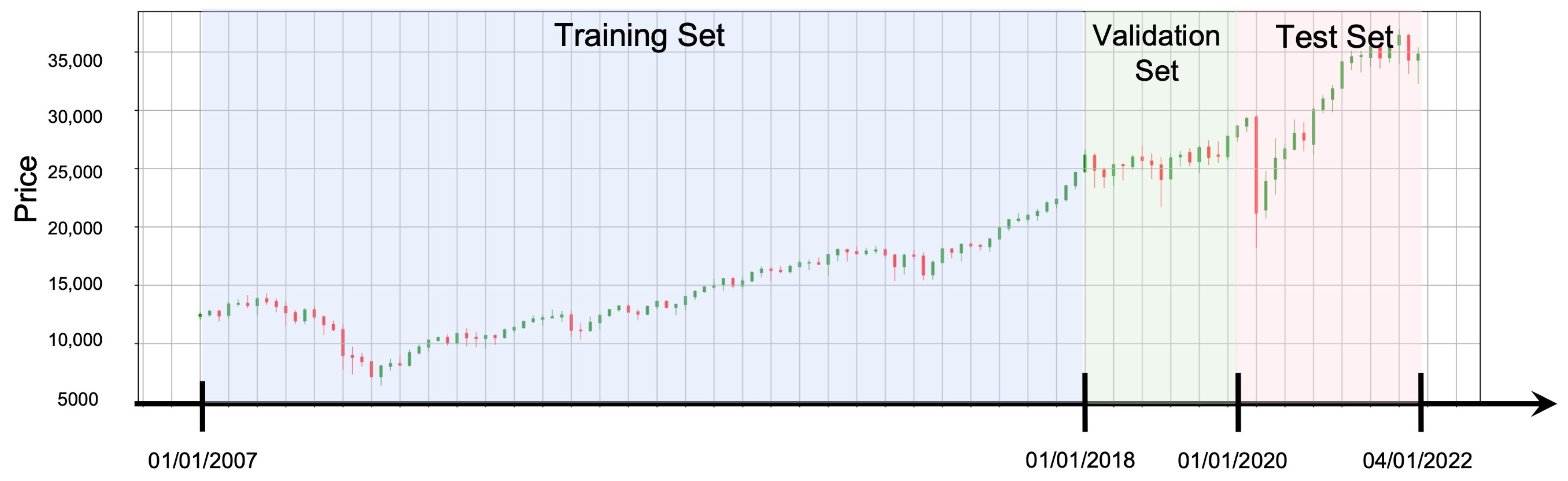
4.1. Data Selection and Preprocessing

This paper conducts a variety of tests to validate our proposed models by using the component stock of DJIA. Our original input data consist of the OHCLV and technical indicators. The OHCLV data utilized for this study are accessible on Yahoo Finance. Technical indicators characterize the market from several viewpoints, and the types and quantities of indicators used for this research are displayed in

Table 1. Summary of financial technical indicators.

Type	Name	Number
Moving averages	Simple Moving Average (SMA), Exponential Moving Average (EMA), Weighted Moving Averages (WMA), Bollinger Bands (BBANDS)	4
Volatility	Average True Range (ATR), True Range (TRANGE), Ulcer Index (UI)	3
Trend	Moving Average Convergence Divergence (MACD), Volatility Ratio (VR), Schaff Trend Cycle (STC), Days Payable Outstanding (DPO), Triple Exponential Average (TRIX), Know Sure Thing (KST)	6
Momentum	Relative Strength Index (RSI), Awesome Oscillator (AO), True Strength Index (TSI), Average Directional Index (ADX), Aroon Oscillator (AROON), Money Flow Index (MFI), Momentum (MOM), Rate of Change (ROC), Williams %R (WILLR), Stochastic (STOCH), Elder Ray Index (ERI)	11
Volume	On-Balance Volume (OBV), Force Index (FI), Accumulation/Distribution (AD), Ease of Movement (EM), Chaikin Money Flow (CMF), Volume Price Trend (VPT), Negative Volume Index (NVI)	7
Total	-	31

and calculated using Talib. Figure 1 depicts the division of our data set into three sections. The data from 1 January 2007 to 1 January 2018 are used for training, and the data from 1 January 2018 to 1 January 2020 are utilized for parameter validation and adjustment. The final test period ran from 1 January 2020 to 1 April 2022. Figure 1 also displays the DJIA’s trend across the whole timespan. We chose a lengthy and volatile period to ensure that the robustness and risk management skills of our trained agents are thoroughly examined. In order to utilize a long-term training set, we eliminated “V” and “DOW” from our portfolio.

For data preprocessing, we implemented a basic Z-score calculation with a rolling window. Specifically, we created a locally standardized characteristic matrix for the s-size rolling window and fed it into the neural network to enable RL agents to efficiently learn. The matrix of local standardized characteristics is defined as follows:

$$X_t=\left(\begin{array}{cccc}\frac{x_{\left(1,t-s+1\right)}}{x_{\left(1,t\right)}}& \frac{x_{\left(1,t-s+2\right)}}{x_{\left(1,t\right)}}& \dots & 1\\ \frac{x_{\left(2,t-s+1\right)}}{x_{\left(2,t\right)}}& \frac{x_{\left(2,t-s+2\right)}}{x_{\left(2,t\right)}}& \dots & 1\\ \dots & \dots & \dots & \dots \\ \frac{x_{\left(m,t-s+1\right)}}{x_{\left(m,t\right)}}& \frac{x_{\left(m,t-s+2\right)}}{x\left(m,t\right)}& \dots & 1\end{array}\right)$$

(3)

where $X_t$ represents one of the OHCLV data and technical indicators.

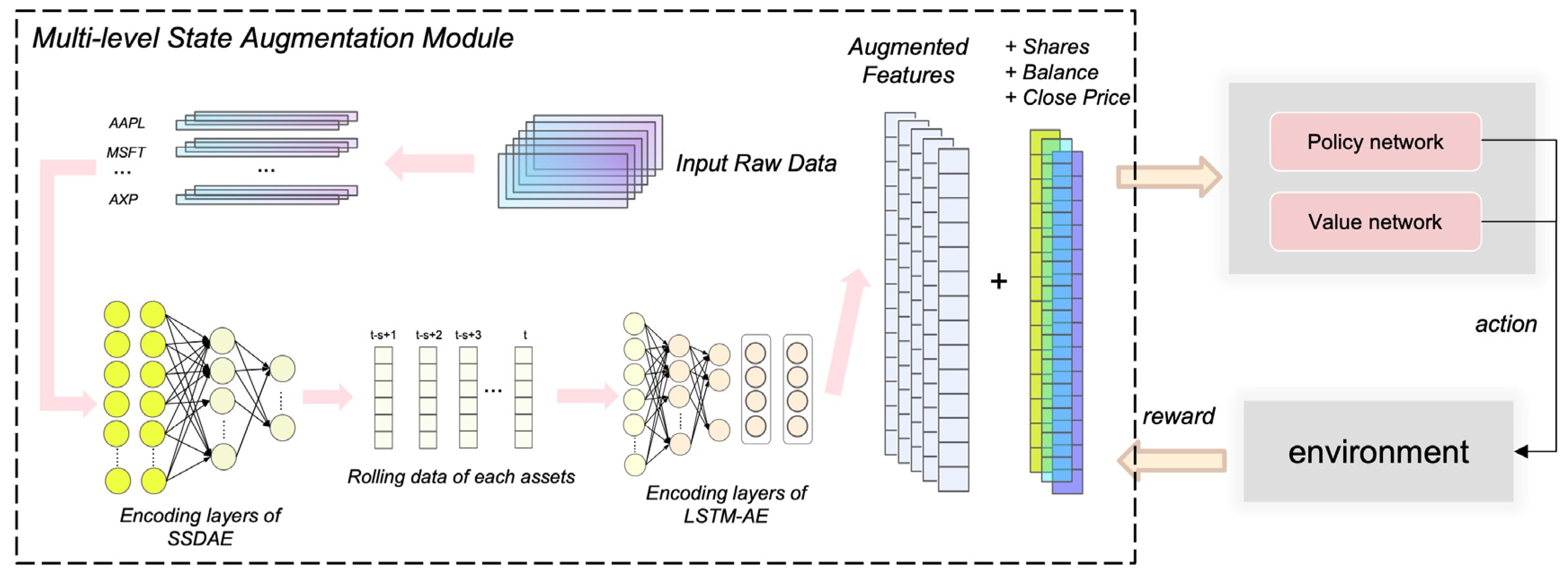
4.2. Multi-Level Augmented Portfolio-Management Model

Our model consists of two components. In the first section, multi-level augmentation was performed on raw financial data to be fed into the state space, and in the second section, the advantage actor–critic algorithm (A2C) was executed. SwanTrader processes each T round in four steps: (1) input of price data and technical indicators; (2) utilizing the MSA to enhance the feature quality and feed the augmented features into the state space; (3) outputting the action, that is, the volume of buy and sell of each stock in the portfolio; and (4) introducing the omega ratio to calculate reward and update the actor network’s trading rules based on the reward. The structure of the SwanTrader is shown in Figure 2.

As depicted in Figure 3, our MSA consists of two steps: extracting robustness information using the SSDAE network and utilizing the LSTM-AE to collect temporal patterns and historical information based on the previous observations. The SSDAE and LSTM-AE networks were trained offline through the training set prior to the trading process, and only encoding layers were used to output informative features in the online trading process.

4.3. Research Models

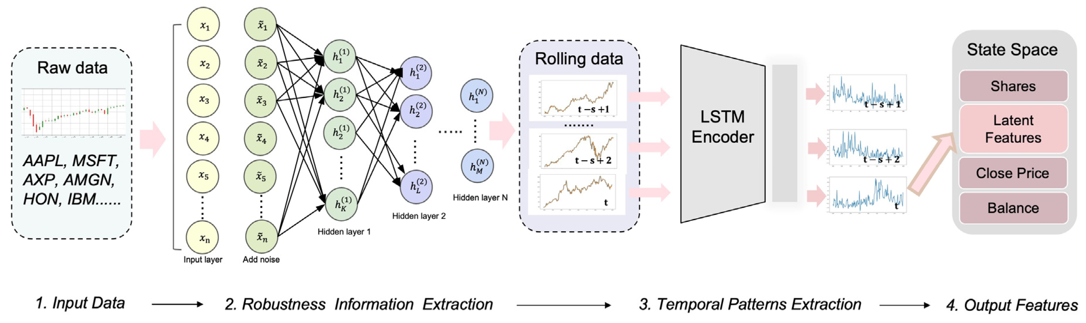
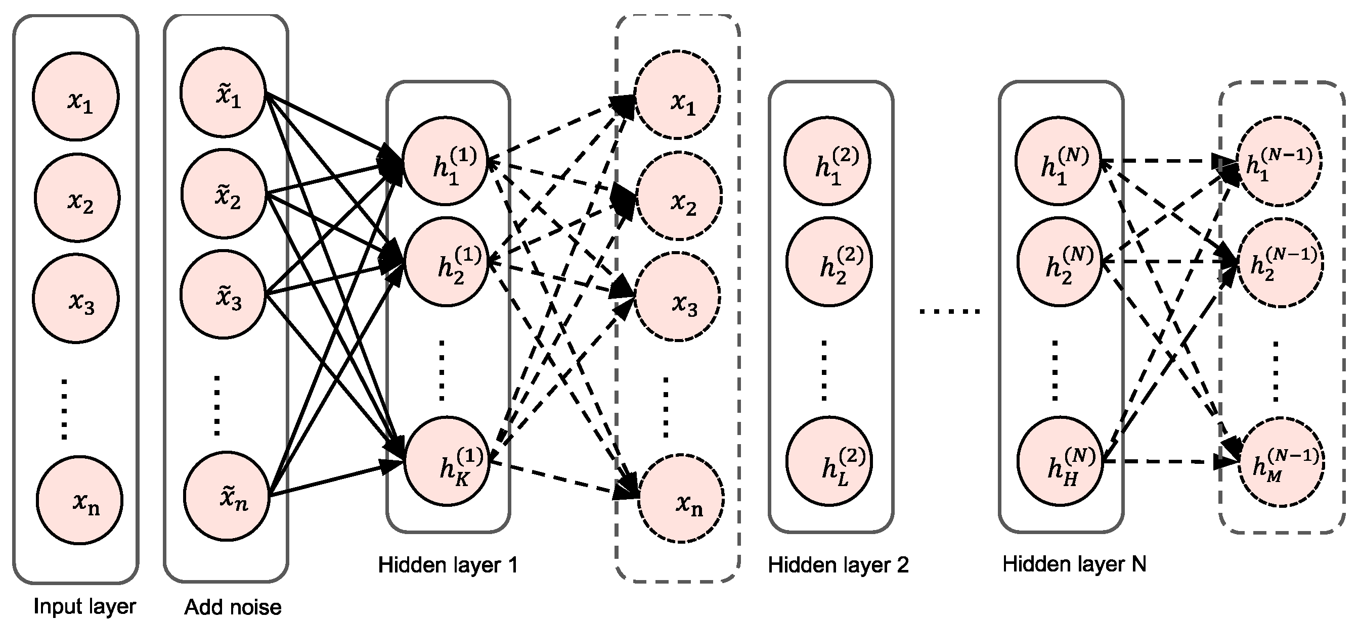
4.3.1. Stacked Sparse Denoising Autoencoder (SSDAE)

We utilized a stacked sparse denoising autoencoder (SSDAE) network to extract latent information to address the issues of high volatility, low signal-to-noise ratio, and external shock of financial data as well as the dimensional disaster caused by the high-dimension state space, which included OHCLV (open, high, close, low, volume) data and a vast number of technical indicators. Our inspiration is derived from past works: Reference [25] employed stacked denoising autoencoders (SDAEs), and reference [22] introduced a constrained stacked autoencoder for dimension reduction. In contrast, we inserted sparse terms, tested a range of network designs, and evaluated a structure for feature augmentation with superior performance under our model. The structure of the SSDAE autoencoder network is depicted in Figure 3. $x_i$ indicates the input data of the ith node, and $h_k^{\left(i\right)}$ represents the input data of the kth node of the ith hidden layer. The arrow in the network diagram reflects the weight of the connection between two neighboring layer nodes. The autoencoder (AE) [52] is a type of unsupervised machine learning that seeks to duplicate the input information using the hidden layer’s learned representation by setting the output values to match the input values. The AE can be viewed as a neural network with three layers. Given the raw training data set $D=\{(x_i\}$, where $i=1,2,\dots m$, m represents the figure for training samples. Following the weighted mapping algorithm, the feature vector for the hidden layer is $h=\left\{h_1,h_2,\cdots ,h_n\right\}$.

$$h=f_{\theta }\left(x\right)=s\left(Wx+b\right)$$

(4)

where $\theta =\left\{W^{\prime },b^{\prime },W,b\right\}$ is the set of the weights matrix and biases vector, and $s\left(t\right)=\left(1+\exp {\left(-t\right)}^{-1}\right)$ is the sigmoid function. Afterward, the hidden layer is inversely mapped, and the reconstructed output vector $z=\left\{z_1,z_2,\cdots ,z_n\right\}$ is by means of Equation (3), and this process is referred to as decoding.

$$z=g_{\theta }\left(h\right)=s\left(W^{\prime }h+b^{\prime }\right)$$

(5)

where $\theta$ are initialized with arbitrary values, and z is an estimate of x.

The objective of training is to minimize the following average squared reconstruction error, and we do this by using J($W$, b) to represent the cost function of AE in relation to all training data presented in:

$$J_{\mathrm{AE}}\left(W,b\right)=\frac{1}{m}{\displaystyle \sum }_{i=1}^m\left(\frac{1}{2}{\parallel z_{W,b}{(x)}^{\left(i\right)}-x^{\left(i\right)}\parallel }_2^2\right)$$

(6)

The AE depends solely on minimizing reconstruction error for network training, which may result in the network simply learning a replica of the original input. The denoising autoencoder (DAE) [53] is based on the AE and employs the noisy input to improve resilience. With the DAE, the expected potential representation has certain stability and resistance in the case of input corruption, so that trading tasks can be conducted more effectively. The initial input $x$ is corrupted into $\tilde{x}$ via a stochastic mapping, and the corrupted input $\tilde{x}$ is then mapped to a hidden representation, and the cost function of DAE is as follows:

$$J_{\mathrm{DAE}}\left(W,b\right)=\frac{1}{m}{\displaystyle \sum }_{i=1}^m\left(\frac{1}{2}{\parallel z_{W,b}{(\tilde{x})}^{\left(i\right)}-x^{\left(i\right)}\parallel }_2^2\right)+\frac{\lambda }{2}({\parallel W\parallel }_F^2+{\parallel W^{\prime }\parallel }_F^2)$$

(7)

where λ is the parameter for the weight decay term.

The SAE adds an additional restriction on the AE, ${\widehat{\rho }}_j=\rho$. The network units are randomly triggered to inhibit some neurons in the hidden layer in order to speed up the updating of network parameters. $\rho$ represents the sparsity term. The objective function adds a new penalty element, relative entropy (Kullback–Leibler divergence), which calculates the difference between two distributions, to achieve this restriction. Equation (7) illustrates the principle:

$$\mathrm{KL}\left(\rho \parallel {\widehat{\rho }}_j\right)=\rho \log \frac{\rho }{{\widehat{\rho }}_j}+\left(1-\rho \right)\log \frac{1-\rho }{1-{\widehat{\rho }}_j}$$

(8)

where KL is expressed in $\rho$, and ${\widehat{\rho }}_j$ is the relative entropy between two Bernoulli random variables with mean value; when ${\widehat{\rho }}_j=\rho$, $\mathrm{KL}\left(\rho \parallel {\widehat{\rho }}_j\right)=0$, and the size of KL increases with the difference between $\rho$ and ${\widehat{\rho }}_j$ increasing monotonically; and when ${\widehat{\rho }}_j$ approaches 0 or 1, the relative entropy becomes infinite; hence, minimizing the penalty factor can cause ${\widehat{\rho }}_j$ approaches $\rho$. Then, an additional penalty term should be introduced to the DAE to meet the sparsity objective, and the sparse denoising autoencoder (SDAE) is trained through:

$$J_{\mathrm{SDAE}}\left(W,b\right)=\frac{1}{m}{\displaystyle \sum }_{i=1}^m\left(\frac{1}{2}{\parallel z_{W,b}{(\tilde{x})}^{\left(i\right)}-x^{\left(i\right)}\parallel }_2^2\right)+\beta {\displaystyle \sum }_{j=1}^s\mathrm{KL}\left(\rho \parallel {\tilde{\rho }}_j\right)+\frac{\lambda }{2}({\parallel W\parallel }_F^2+{\parallel W^{\prime }\parallel }_F^2)$$

(9)

where $\beta$ indicates the sparsity term parameter.

Multiple single-layered autoencoders are piled together to create a deep neural model, which is often used to improve the learning capacity of autoencoder networks. The stacked AE network structure with N hidden layers is shown in Figure 4. Currently, the stacked AE network utilizes the greedy layer-by-layer training strategy [52], which mitigates the step dispersion phenomenon to some degree. The stacked autoencoder is trained without supervision. The output of the first hidden layer is then used to pre-train the second hidden layer. This process is repeated for each subsequent layer. After pre-training all layers, the encoding network in each layer is removed, leaving only the decoding network. The entire stacked network is then fine-tuned using gradient descent until the optimal network parameters have been determined. The SSDAE network transforms the original input into the extracted characteristics of the nth layer. During the phase of fine-tuning, the loss function of the SSDAE network is as follows:

$$J_{\mathrm{SSDAE}}\left(W,b\right)=\frac{1}{m}{\displaystyle \sum }_{i=1}^m\left(\frac{1}{2}{\parallel h_{W,b}{(\tilde{x})}^{\left(i\right)}-x^{\left(i\right)}\parallel }_2^2\right)+\frac{\lambda }{2}{\displaystyle \sum }_{l=1}^{2l}({\parallel W_l\parallel }_F^2)$$

(10)

where $W_l$ is the weight of the lth SSDAE layer. Since the pretrained weights would be used as regularization in our network, the sparsity term was deleted.

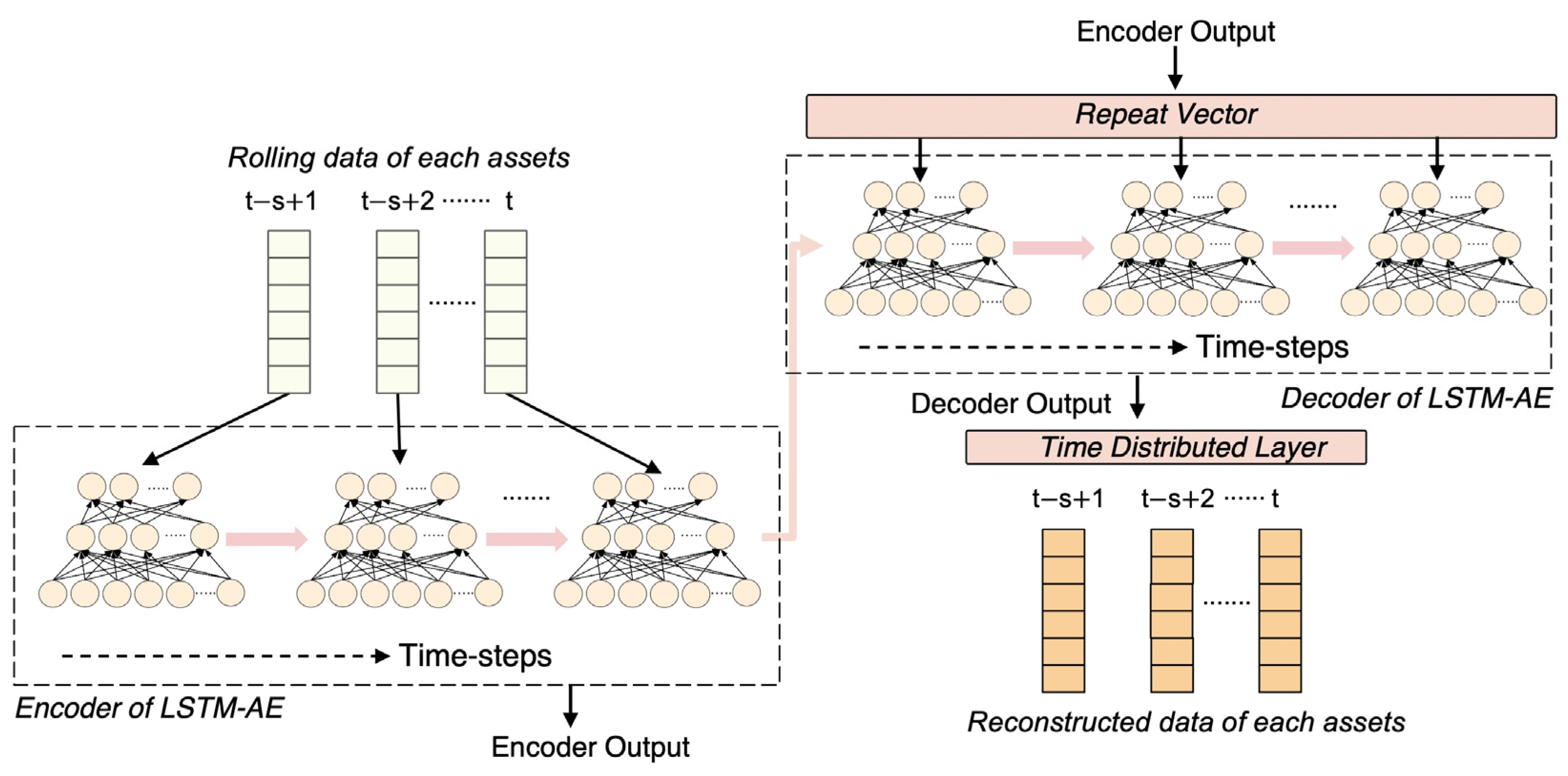
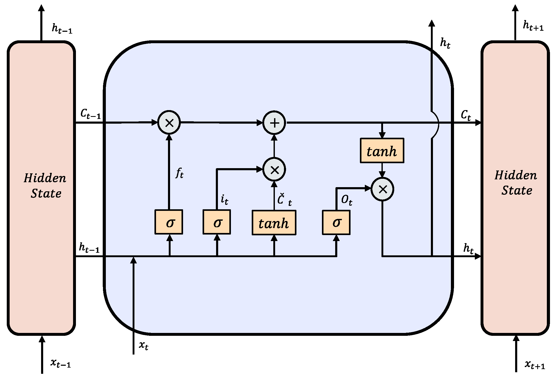
4.3.2. Long–Short-Term-Memory-Based Autoencoder (LSTM-AE)

The long–short-term-memory (LSTM) network is intended for sequential data processing. Due to its exceptional ability in retaining correlations between temporal sequences, the LSTM [54] has been extensively utilized to capture temporal patterns, such as stock market trend [55,56,57]. For decision making, RL agents only utilize the most current state data. Taking into account that LSTM networks can store state information prior to network input, the retrieved potential features contain historical data. In order to replicate the input sequence, the LSTM-AE is typically trained in the same manner as the AE model, and the reconstructed loss function is identical to that of a basic AE network. The encoder network discovers a fixed-length vector format from the time-series input data. This representation is utilized by the decoder network to reconstruct the time series using the previously predicted value and the current hidden state. The LSTM-AE structure is shown in Figure 5.

A LSTM unit is depicted in Figure 6. The LSTM cell structure controls the update and utilization of historical information mainly through three gates, thereby overcoming the vanishing gradient problem: input gate $i_t$ regulates the reading of fresh data, forget gate $f_t$ controls the erasure of data, and output gate $O_t$ controls the transmission of data. The following equations illustrate the LSTM operation:

$$f_t=\sigma \left(W_f\cdot \left[h_{t-1},x_t\right]+b_f\right)$$

(11)

$$i_t=\sigma \left(W_i\cdot \left[h_{t-1},x_t\right]+b_i\right)$$

(12)

$$O_t=\sigma \left(W_o\cdot \left[h_{t-1},x_t\right]+b_o\right)$$

(13)

$$\begin{array}{cc}\check{C_t}& =\tan \mathrm{h}\left(W_C\cdot \left[h_{t-1},x_t\right]+b_C\right)\end{array}$$

(14)

$$C_t=f_t\times C_{t-1}+i_t\times \check{C_t}$$

(15)

$$h_t=O_t\times \tan \mathrm{h}\left(C_t\right)$$

(16)

where $C_t$ indicates the cell state, $\check{C}{}_t$ indicates a vector of newly generated candidate values by a tanh layer, $x_t$ indicates the input data, $h_t$ is the output data, W and b represent the weights and biases respectively, and the × represents element-by-element multiplication.

4.3.3. Optimization Algorithms—Advantage Actor–Critic (A2C)

In this study, we employed one of the actor–critic algorithms, the advantage actor–critic (A2C), which prior research has shown to outperform other DRL algorithms in quantitative management tasks [44,58,59]. We implemented it using stable-baselines3 [46]. The A2C algorithm [60] presented by OpenAI is a variant of the asynchronous advantage actor–critic (A3C) algorithm [61]. A2C reduces the variance of the policy gradient by utilizing an advantage function. We updated our policy based on the objective function:

$$\nabla J_{\theta }\left(\theta \right)=\mathbb{E}\left[{\displaystyle \sum }_{t=1}^T{\nabla }_{\theta }\log {\pi }_{\theta }\left(a_t\mid s_t\right)A\left(s_t,a_t\right)\right]$$

(17)

where ${\pi }_{\theta }\left(a_t\mid s_t\right)$ denotes the policy network parameterized by θ, and $A\left(s_t,a_t\right)$ indiactes the advantage function defined as follows:

$$A\left(s_t,a_t\right)=q_{\pi }\left(s_t,a_t\right)-V_{\pi }\left(s_t\right)=r\left(s_t,a_t,s_{t+1}\right)+\gamma V_{\pi }\left(s_{t+1}\right)-V_{\pi }\left(s_t\right)$$

(18)

where $q_{\pi }\left(s,a\right)$ represents the expected reward at state $s_t$ when taking action $a_t$, and $V_{\pi }$ ($s_t$) is the value function.

The OpenAI gym [62] serves as the foundation for our portfolio trading environment. A2C is employed by using stable-baselines3 [46]. The size of the input sliding window is set to 20, the transaction cost rate λ is set to 0.2%, the time steps for each update are set to 5, the maximum value of gradient clipping is to 0.5, and the learning rate is to 0.0001. To prevent insufficient learning, such as local minimum and overfitting, gradient clipping is used, and our A2C actor network employs the Adam optimizer, which has been demonstrated in trials to enhance the training stability and convergence speed of the DRL model [63].

4.3.4. Setting of Reward Function

Typically, the formulation of the reward function is a difficult step in the design of a reinforcement learning problem. In reality, the return on an investor’s management is the change in their stock portfolio’s value that evening. In terms of RL, the reward is a profit or loss resulting from the action between states $s_t$ and $s_{t+1}$, as described by the reward function Equation (19).

$$r\left(s_t,a_t,s_{t+1}\right)=R_{t+1}-R_t-c_t$$

(19)

where $R_t=b_{t+1}+p_{t+1}^T{h}_{t+1}$ represents the portfolio value at t + 1 and t, respectively; the portfolio value is the total stock value plus the balance $c_t$ indicates the transaction cost, $p_t$ indicates the vector of the price of trading shares for the stocks in each step, and $p_t^T$ represents the transpose of matrix.

Despite the transaction costs, which can take many different shapes and are billed in various ways, this paper assumes our transaction costs to be a fixed proportion λ of the value of each trade (either buy or sell), as in [59]:

$$c_t=p^T{\sum }_{d=1}^D\left|k_t\right|\times \lambda$$

(20)

where $k_t$ represents the vectors of the stocks’ trading share numbers at each step.

In the real world, we commonly use the change rate of the portfolio value to judge profit and loss. However, it is challenging to offer consistent commentary on using this type of reward function. We suggest modifying the reward as follows by using the extra trade return:

$$Adj\_T{r}_t^s=ln\left(\frac{\left[\left(R_t-d_t\right)-\left(R_{t-s}-d_t\right)\right]}{R_{t-s}-d_t}\right)$$

(21)

where $Adj\_T{r}_t^s$ represents the realized logarithmic rate of excess trade return in a period of time t, the length of period is s, and $d_t$ represents the rate of the return of the baseline. The Dow Jones industrial average (DJIA) index serves as the reference point in this paper.

Moreover, this paper developed a novel reward function based on the omega ratio. The probability weighted ratio of return to loss under a specific predicted return level is known as the omega ratio. The omega ratio is seen to be a stronger performance indicator than the Sharpe ratio, Sortino ratio, and Calmar ratio since it depends on the distribution of all returns and thus contains all information regarding risks and returns [32]. The formula is described as follows:

$$O{r}_t=\frac{{{\displaystyle \int }}_{d_t}^{\infty }\left(1-F\left(x\right)\right)dx}{{{\displaystyle \int }}_{-\infty }^{d_t}F\left(x\right)dx}=\frac{{\sum }_{d=1}^D\left|k_t\right|}{{{\displaystyle \int }}_{-\infty }^{d_t}F\left(x\right)dx}$$

(22)

where $F\left(x\right)$ indicates the cumulative distribution function of $T{r}_t^1$ in an s-size period ($Adj\_T{r}_t^1$ is the daily return).

5. Experimental Setup and Results

5.1. Parameters of Network

Several preliminary evaluations are carried out to find the better AE network parameters. The input dimension is 36 (the number of OHCLV data is 5, and the number of technical indicators is 31). The sparsity is applied up to 10⁻⁸, and the regularization term is set as 10⁻⁵; the epoch of pre-training is 100, and the epoch of fine-tuning is 200; the average value of loss function of the SSADE on the training set is treated as the objective. Thus, the SSDAE captures the most robustness information, and the utilized structure is [36-48-64-128-64-48-36]. As for the LSTM network parameters, such as the number of hidden layers and the number of LSTM units for each layer, the network topology is achieved as [128-32-4-32-128], and 100 LSTM units for each layer are selected as the network parameters in this paper. The mean square error (MSE) between the true target value and the estimated target value is employed as the loss function. The ReLU is set as the activation function. The Adam optimizer is applied to update the weight and bias values and mitigate the gradient explosion problem. The learning is applied up to 120 epochs for training the network. For the above two AE networks, to prevent inadequate learning, the gradient clipping is all implemented through the grad_clip_norm in PyTorch, and we set the value as 10, and the L2 regularization term of weight (REG_LAMBDA) is set to 0.01.

5.2. Metrics

Six metrics are used in our experiments, which can be divided into three types: (1) profit metric, including accumulative rate of return (ARR) and alpha; (2) risk metric, including maximum drawdown (MDD) and beta; and (3) risk-profit metric, including Sharpe ratio (SR) and Calmar ratio (CMR). The ARR is a common metric used to evaluate strategic profits, and the greater the cumulative return, the greater the strategy’s profitability. The SR reflects the additional amount of return an investor receives for each unit of risk. The MDD is metric to assess the potential loss that seeks the maximum change from the highest to the lowest. The CMR [64] is used to measure the risk by using the concept of MDD, and the higher the Calmar ratio, the better it performed on a risk-adjusted basis. Alpha, commonly regarded as the active return, compares the performance of an investment to a market index or benchmark that is considered to represent the market’s overall movement. The calculation process of the alpha value is shown in:

$$\mathrm{Alpha}=R_p-\left[R_f+{\beta }_p\left(R_m-R_f\right)\right]$$

(23)

where $R_p$ is the yield of the model, ${\beta }_p$ is the beta value of the model, and $R_m$ is the yield of the benchmark strategy. Beta is widely employed as a risk-reward statistic that enables investors to assess how much risk they are willing to assume in exchange for a certain return. The formula is illustrated below:

$$\mathrm{Beta}=\mathrm{Cov}\left(R_p,R_m\right)/{\sigma }_m^2$$

(24)

where $\mathrm{Cov}$ is the covariance, and ${\sigma }_m^2$ is the variance of the benchmark strategy.

5.3. Baselines

The comparison models described below are trained and traded under the same trading environment, trading rules, and parameters.

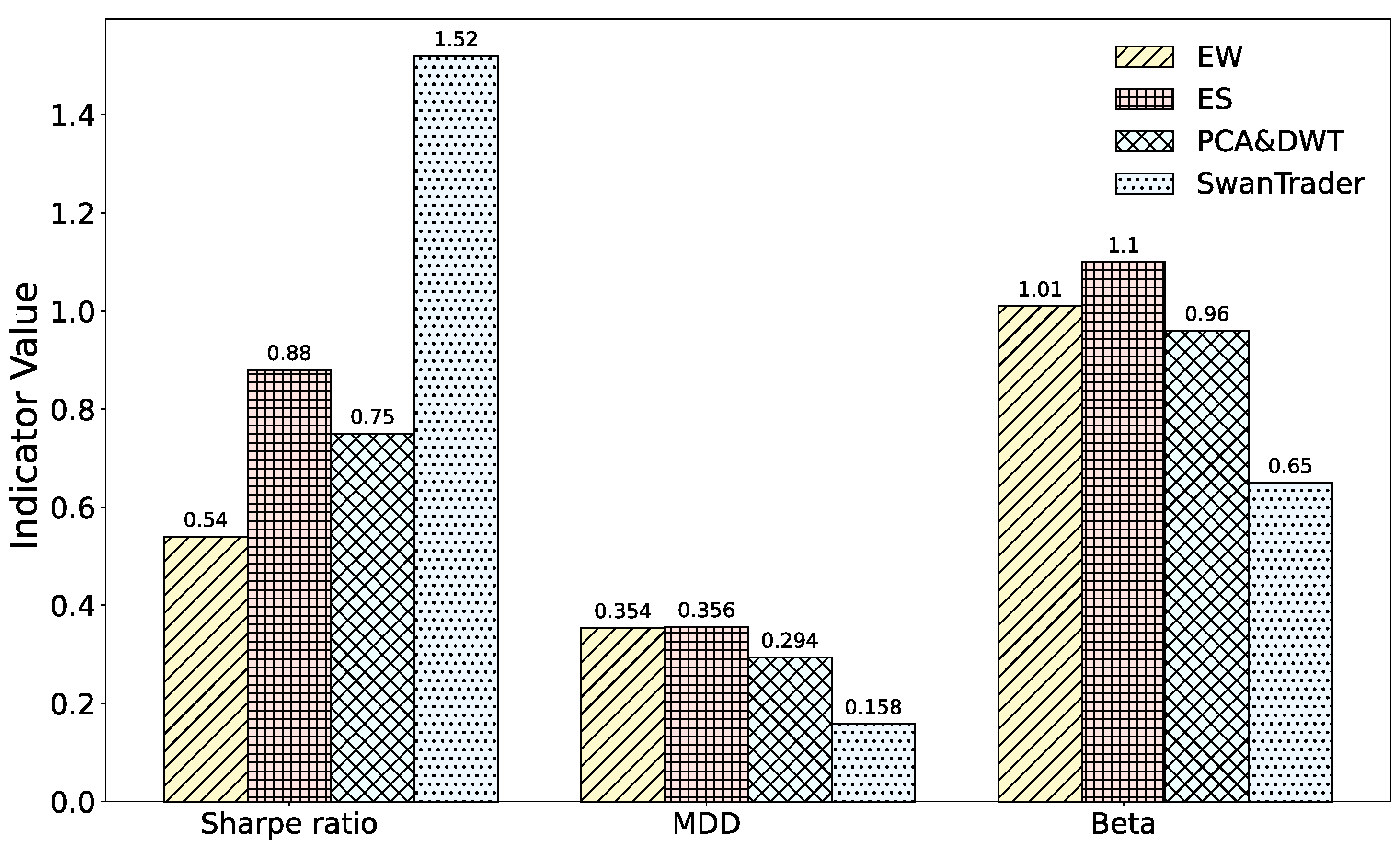
• EW (Equal weight baseline): a simplistic baseline that allocates equal weight to all portfolio assets;
• Anticor (Anti-Correlation) [65]: a heuristic technique for online portfolio selection that uses the consistency of positive lagged cross-correlation and negative autocorrelation to change portfolio weights according to the mean regression principle;
• CRP (Constant rebalanced portfolio) [66]: an investing strategy that maintains the same wealth distribution among a collection of assets on a daily basis, that is, the fraction of total wealth represented by a particular asset remains constant at the start of each day;
• CORN (CORrelation-driven nonparametric learning) [67]: a model for correlation-driven nonparametric learning that combines correlation sample selection with logarithmic optimal utility function;
• ONS (Online newton step algorithm) [68]: an online portfolio selection model based on the newton model which requires relatively weak assumptions;
• ES (Ensemble strategy) [69]: a recently developed RL-based open-source model that improves performance by integrating three actor–critic algorithms without the process of state space augmentation;
• PCA and DWT (Principal Component Analysis and Discrete Wavelet Transform) [23]: by combining PCA and DWT to extract features from financial data, it is found that the profitability is better than the setting without feature processing.

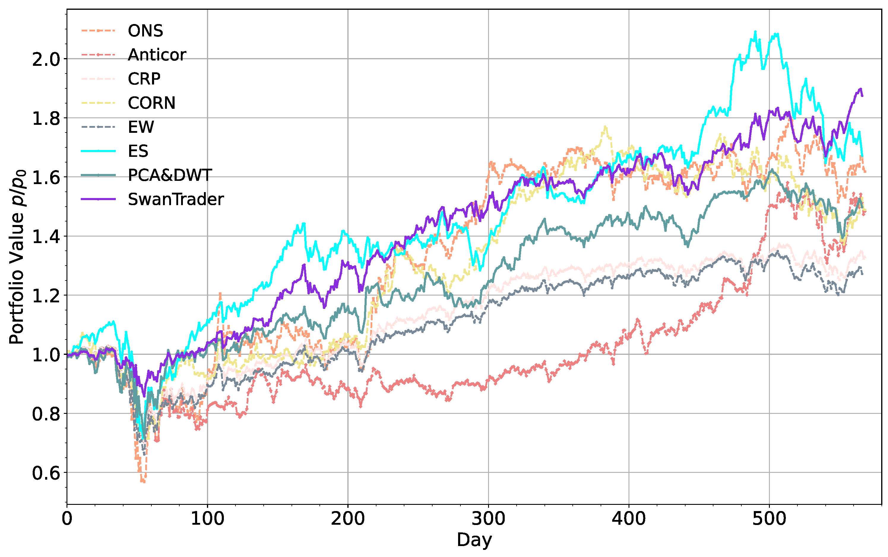
5.4. Result Comparison

To verify the superiority of our proposed approach, we employed some baselines that had been widely used in previous research [5,70,71] for comparative analysis: four online portfolio selection models, two state-of-the-art reinforcement learning-based portfolio-management models, and an equal weight (EW) baseline. Furthermore, we verified the generalization ability of all models using a long time-span dataset (from 1 January 2020 to 1 April 2022). The results tabulated in

Table 2. Evaluation on different models.

Model	ARR (%)	MDD (%)	SR	CMR	Alpha	Beta
EW	27.2	−35.4	0.54	0.32	−0.02	1.01
Anticor	48.4	−33.5	0.67	0.57	0.02	1.08
CRP	32.9	−33.2	0.62	0.40	−0.04	0.98
CORN	48.9	−33.4	0.71	0.58	0.05	0.93
ONS	61.8	−44.0	0.71	0.54	0.04	1.35
ES	67.2	−35.6	0.88	0.72	0.07	1.10
PCA and DWT	49.8	−29.4	0.75	0.67	0.04	0.96
SwanTrader	87.5	−15.8	1.52	2.04	0.19	0.65

and Figure 7 and Figure 8 indicate that the performance of the proposed approach is significantly better than all the models in terms of the accumulative rate of return (ARR), maximum drawdown (MDD), Calmar ratio, Sharpe ratio, and alpha and beta during the testing period. Specifically, SwanTrader achieves an ARR of 87.5%, which is greater by 20.3% than the second-highest approach, ES. The Sharpe ratio of SwanTrader is 1.52, which is 0.64 higher than the second-highest model, ES. The alpha value of SwanTrader is 0.19, which is 0.12 higher than the second-highest model, ES. When COVID-19 broke out, the market plummeted dramatically, and while the majority of trading strategies experienced big losses, the SwanTrader demonstrated the best ability to resist dropping prices. In the beta values and MDD (%), they reached 0.65 and −15.8, respectively. The ONS performs the best in four online portfolio selection models, reaching 61.8% in terms of ARR and −44.0 in MDD (%). However, there is a big gap compared with reinforcement learning-based models in Sharpe ratio and Calmar ratio, which are only 0.71 and 0.54. In conclusion, this demonstrates the superiority of our proposed model over other baselines, and the superior trading performance displayed by the proposed SwanTrader model indicates it not only reduces loss in the downward trend but also captures profits in the upward trend.

6. Analysis and Discussion

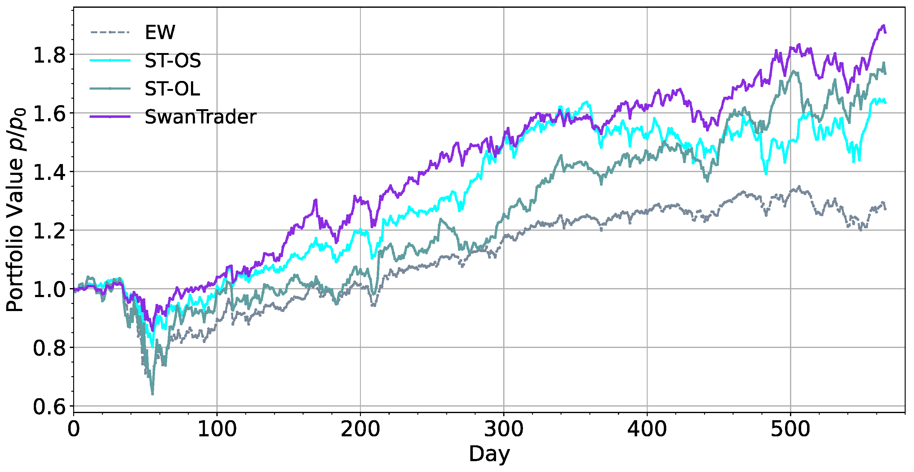
6.1. Effects of Augmentation Network

In order to further evaluate the effectiveness of the proposed model and examine the functions of essential components, we employed two simpler versions of SwanTrader (ST). Firstly, we removed the LSTM-AE network and only employed SSDAE to augment state space features to examine the effect of SSDAE network, named SwanTrader-Only-SSDAE (ST-OS). Similarly, SwanTrader-Only-LSTM-AE (ST-OL) was employed to test the function of LSTM-AE network. As shown in Figure 9 and

Table 3. Effects of augmentation network.

Model	ARR (%)	MDD (%)	SR	CMR	Alpha	Beta
ST-OS	63.6	−22.7	1.03	1.08	0.10	0.77
ST-OL	73.4	−38.4	0.90	0.72	0.09	1.09
SwanTrader	87.5	−15.8	1.52	2.04	0.19	0.65

, compared to the simplified versions (ST-OS and ST-OL), our strategy achieved a better balance between benefits and risks for all measurement indicators with SwanTrader. In the experiment including the disassembly of the two components, the result indicates that ST-OS is more profitable by 73.5%, showing that the LSTM-AE network can capture the temporal pattern to some extent. However, this results in high MDD values (−38.4%), a risk that is unacceptable to many investors. ST-OS performs the worst in terms of ARR (63.6%), but it outperforms ST-OL in terms of Sharpe ratio and Calmar ratio due to low MDD values (22.7%), indicating that the higher-level features augmented by the SSDAE network improve agents’ risk aversion. Thus, the results show that the SSDAE network contributes to higher risk-control ability, and LSTM-AE network is conducive to higher profit and loss. By integrating these two modules, we obtain the MSA we proposed, which not only assists agents in mitigating losses during a downturn but also ensures greater revenues during an upturn.

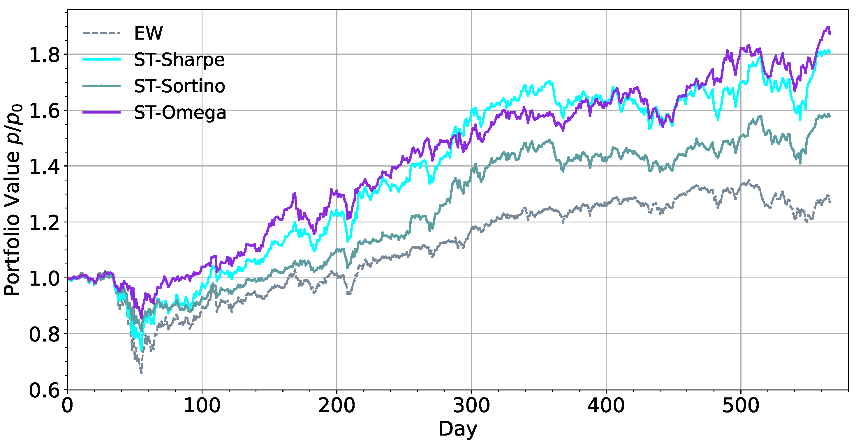
6.2. Effects of Reward Function

To determine the effect of using the omega ratio as the default reward function in the proposed model, we employed the Sharpe ratio, Calmar ratio [29], and Sortino ratio [28] as alternative choices of reward functions in SwanTrader, which are utilized for portfolio management in previous works [24,25,26,28,29]. Compared with the technical indicators that only using the second moment or MDD, the omega ratio depends on the distribution of all returns and therefore contains all risk and return information. As presented in Figure 10 and

Table 4. Effectiveness of Omega Ratio.

Model	ARR (%)	MDD (%)	SR	CMR	Alpha	Beta
ST-Sharpe	80.7	−26.4	1.17	1.14	0.14	0.84
ST-Sortino	57.8	−19.5	1.21	1.15	0.12	0.56
SwanTrader	87.5	−15.8	1.52	2.04	0.19	0.65

, ST-Sharpe is more profitable with a higher ARR than ST-Sortino, hitting 80.7. ST-Sharpe performed poorly on MDD values (−26.4) and had inferior SR and CMR compared to ST-Sortino. ST-Sortino utilizes the Sortino ratio as the reward, which only factors in the negative deviation of a trading strategy’s returns from the mean and helps to achieve better MDD (−19.5) and beta (0.56) values. The result indicates that only adding downward information in reward function contribute to improve the performance during the downtrend. ST-Sortino has better risk-control ability in terms of MDD but at the expense of profitability; ARR is only 57.8%, which is 22.9% less than ST-Sharpe. Finally, using the omega ratio as the reward function achieves the best results in all measurements. The results show that the omega ratio is conducive to obtaining a low MDD while maintaining a reasonably high return, which is an ideal reward function setting.

7. Conclusions

This paper built a Markov decision process model-based deep reinforcement learning model for quantitative portfolio management in times of COVID-19. In detail, by using OHCLV data and financial technical indicators for each asset, this paper employed a stacked sparse denoising autoencoder (SSDAE) model and a long–short-term-memory-based autoencoder (LSTM-AE) model to analyze and capture the temporal patterns and robustness information based on market observations; A2C was used to optimize and output sequence decisions. Additionally, using two simplified structures of our suggested model and three types of reward function, namely Sharpe ratio, Sortino ratio, and omega ratio, we explored the role of these settings in our suggested model. This paper also compares our model with five standard machine learning models (Anticor, CRP, CORN, ONS) and two state-of-the-art reinforcement learning models (ES [69] and PCA and DWT [23]). According to the back-test results during the COVID-19 pandemic, we can conclude that:

(1)

The DRL-based portfolio-management model outperforms other standard machine learning-based models in terms of Sharpe ratio, Sortino ratio, and MDD, which means that Markov decision process model is more suitable than supervised learning by allowing the tasks of “prediction” and “portfolio construction” to be combined in one integration step.

(2)

By introducing deep learning into the Markov decision process model and adjusting network structural parameters, the suggested model has a positive effect on balancing risk and profit. This is the same as the conclusion of Li [23] and Ren [72].

(3)

Through the ablation study, it can be seen that SSDAE model has a significant effect on risk control, especially in the volatility and drawdown of model; the LSTM-AE model has a significant effect in capturing market trends, but it will also increase losses while increasing profits. By integrating the two models, we can obtain a better balance between risk and return.

(4)

We also found that the choice of reward function will also affect the risk preference of the model. By comparing the trading returns, Sharpe ratio, Sortino ratio, and omega ratio, we found that the more accurate assessment of the value of risk penalty means that the model has a greater tendency to output prudent action.

To conclude, this paper extends the Markov process model literature by serving as an attempt toward developing a quantitative portfolio-management model using a deep-learning-based reinforcement learning method. The result indicates that inputting augmented state space features improves the performance of the proposed portfolio-management model. The advantages of the suggested model are its scalability and applicability. Furthermore, the model’s consistent performance on a long time-span dataset indicates that it is generalizable.

Nonetheless, there are certain restrictions in this study. To examine the effects of the proposed model on portfolio-management performance, features from external financial environments such as social news and other types of macro data should be exploited, and its interpretability regarding feature augmentation approach requires more discussion. Our study indicates the viability of application of the deep learning models in portfolio management. More deep learning models are also promising for further improving the strategy performance of quantitative portfolio management.

The results of our suggested model for investors can assist in reducing the risk of investment loss as well as help them to make sound decisions. In future research, in consideration of correlations between financial assets, it is possible to extend the proposed model to exploit cross-asset dependency information and use more comprehensive risk measurement tools, such as value-at-risk [73] and conditional-value-at-risk [74].

References

1. Wolf, P.; Hubschneider, C.; Weber, M.; Bauer, A.; Härtl, J.; Dürr, F.; Zöllner, J.M. Learning How to Drive in a Real World Simulation with Deep Q-Networks. In Proceedings of the 2017 IEEE Intelligent Vehicles Symposium (IV), Los Angeles, CA, USA, 11–14 June 2017; IEEE: Piscataway, NJ, USA, 2017; pp. 244–250. [Google Scholar]
2. Ye, D.; Liu, Z.; Sun, M.; Shi, B.; Zhao, P.; Wu, H.; Yu, H.; Yang, S.; Wu, X.; Guo, Q. Mastering Complex Control in Moba Games with Deep Reinforcement Learning. In Proceedings of the AAAI Conference on Artificial Intelligence, New York, NY, USA, 7–12 February 2020; Volume 34, pp. 6672–6679. [Google Scholar]
3. Silver, D.; Schrittwieser, J.; Simonyan, K.; Antonoglou, I.; Huang, A.; Guez, A.; Hubert, T.; Baker, L.; Lai, M.; Bolton, A.; et al. Mastering the Game of Go without Human Knowledge. Nature 2017, 550, 354–359. [Google Scholar] [CrossRef] [PubMed]
4. Yu, Z.; Machado, P.; Zahid, A.; Abdulghani, A.M.; Dashtipour, K.; Heidari, H.; Imran, M.A.; Abbasi, Q.H. Energy and Performance Trade-off Optimization in Heterogeneous Computing via Reinforcement Learning. Electronics 2020, 9, 1812. [Google Scholar] [CrossRef]
5. Wang, R.; Wei, H.; An, B.; Feng, Z.; Yao, J. Commission Fee Is Not Enough: A Hierarchical Reinforced Framework for Portfolio Management. arXiv 2020, arXiv:2012.12620. [Google Scholar]
6. Jiang, Z.; Liang, J. Cryptocurrency Portfolio Management with Deep Reinforcement Learning. In Proceedings of the 2017 Intelligent Systems Conference (IntelliSys), London, UK, 7–8 September 2017; IEEE: Piscataway, NJ, USA, 2017; pp. 905–913. [Google Scholar]
7. Liang, Q.; Zhu, M.; Zheng, X.; Wang, Y. An Adaptive News-Driven Method for CVaR-Sensitive Online Portfolio Selection in Non-Stationary Financial Markets. In Proceedings of the Thirtieth International Joint Conference on Artificial Intelligence, International Joint Conferences on Artificial Intelligence Organization, Montreal, QC, Canada, 19–26 August 2021; pp. 2708–2715. [Google Scholar]
8. Yang, H.; Liu, X.-Y.; Zhong, S.; Walid, A. Deep Reinforcement Learning for Automated Stock Trading: An Ensemble Strategy. In Proceedings of the First ACM International Conference on AI in Finance, New York, NY, USA, 15–16 October 2020; pp. 1–8. [Google Scholar]
9. Chen, Y.-F.; Huang, S.-H. Sentiment-Influenced Trading System Based on Multimodal Deep Reinforcement Learning. Appl. Soft Comput. 2021, 112, 107788. [Google Scholar] [CrossRef]
10. Liu, Y.; Liu, Q.; Zhao, H.; Pan, Z.; Liu, C. Adaptive Quantitative Trading: An Imitative Deep Reinforcement Learning Approach. AAAI 2020, 34, 2128–2135. [Google Scholar] [CrossRef]
11. Lu, D.W. Agent Inspired Trading Using Recurrent Reinforcement Learning and LSTM Neural Networks. arXiv 2017, arXiv:1707.07338. [Google Scholar]
12. Verleysen, M.; François, D. The Curse of Dimensionality in Data Mining and Time Series Prediction. In Proceedings of the International Work-Conference on Artificial Neural Networks; Springer: Berlin/Heidelberg, Germany, 2005; pp. 758–770. [Google Scholar]
13. Betancourt, C.; Chen, W.-H. Deep Reinforcement Learning for Portfolio Management of Markets with a Dynamic Number of Assets. Expert Syst. Appl. 2021, 164, 114002. [Google Scholar] [CrossRef]
14. Huang, Z.; Tanaka, F. MSPM: A Modularized and Scalable Multi-Agent Reinforcement Learning-Based System for Financial Portfolio Management. PLoS ONE 2022, 17, e0263689. [Google Scholar] [CrossRef]
15. Park, H.; Sim, M.K.; Choi, D.G. An Intelligent Financial Portfolio Trading Strategy Using Deep Q-Learning. Expert Syst. Appl. 2020, 158, 113573. [Google Scholar] [CrossRef]
16. Théate, T.; Ernst, D. An Application of Deep Reinforcement Learning to Algorithmic Trading. Expert Syst. Appl. 2021, 173, 114632. [Google Scholar] [CrossRef]
17. Meng, Q.; Catchpoole, D.; Skillicorn, D.; Kennedy, P.J. Relational Autoencoder for Feature Extraction. In Proceedings of the 2017 International Joint Conference on Neural Networks (IJCNN), Anchorage, AK, USA, 14–19 May 2017; pp. 364–371. [Google Scholar]
18. Yashaswi, K. Deep Reinforcement Learning for Portfolio Optimization Using Latent Feature State Space (LFSS) Module. 2021. Available online: https://arxiv.org/abs/2102.06233 (accessed on 7 August 2022).
19. Jang, J.-G.; Choi, D.; Jung, J.; Kang, U. Zoom-Svd: Fast and Memory Efficient Method for Extracting Key Patterns in an Arbitrary Time Range. In Proceedings of the 27th ACM International Conference on Information and Knowledge Management, Torino Italy, 22–26 October 2018; pp. 1083–1092. [Google Scholar]
20. Taylor, G.W.; Hinton, G.E. Factored Conditional Restricted Boltzmann Machines for Modeling Motion Style. In Proceedings of the 26th Annual International Conference on Machine Learning, Montreal, QC, Canada, 14–18 June 2009; pp. 1025–1032. [Google Scholar]
21. Hinton, G.E.; Salakhutdinov, R.R. Reducing the Dimensionality of Data with Neural Networks. Science 2006, 313, 504–507. [Google Scholar] [CrossRef] [PubMed]
22. Soleymani, F.; Paquet, E. Financial Portfolio Optimization with Online Deep Reinforcement Learning and Restricted Stacked Autoencoder—DeepBreath. Expert Syst. Appl. 2020, 156, 113456. [Google Scholar] [CrossRef]
23. Li, L. An Automated Portfolio Trading System with Feature Preprocessing and Recurrent Reinforcement Learning. arXiv 2021, arXiv:2110.05299. [Google Scholar]
24. Lee, J.; Koh, H.; Choe, H.J. Learning to Trade in Financial Time Series Using High-Frequency through Wavelet Transformation and Deep Reinforcement Learning. Appl. Intell. 2021, 51, 6202–6223. [Google Scholar] [CrossRef]
25. Li, Y.; Zheng, W.; Zheng, Z. Deep Robust Reinforcement Learning for Practical Algorithmic Trading. IEEE Access 2019, 7, 108014–108022. [Google Scholar] [CrossRef]
26. Wu, M.-E.; Syu, J.-H.; Lin, J.C.-W.; Ho, J.-M. Portfolio Management System in Equity Market Neutral Using Reinforcement Learning. Appl. Intell. 2021, 51, 8119–8131. [Google Scholar] [CrossRef]
27. Sharpe, W.F. Mutual Fund Performance. J. Bus. 1966, 39, 119–138. [Google Scholar] [CrossRef]
28. Wu, X.; Chen, H.; Wang, J.; Troiano, L.; Loia, V.; Fujita, H. Adaptive Stock Trading Strategies with Deep Reinforcement Learning Methods. Inf. Sci. 2020, 538, 142–158. [Google Scholar] [CrossRef]
29. Almahdi, S.; Yang, S.Y. An Adaptive Portfolio Trading System: A Risk-Return Portfolio Optimization Using Recurrent Reinforcement Learning with Expected Maximum Drawdown. Expert Syst. Appl. 2017, 87, 267–279. [Google Scholar] [CrossRef]
30. Grinold, R.C.; Kahn, R.N. Active Portfolio Management: Quantitative Theory and Applications; Probus: Chicago, IL, USA, 1995. [Google Scholar]
31. Magdon-Ismail, M.; Atiya, A.F. Maximum Drawdown. Risk Mag. 2004, 17, 99–102. [Google Scholar]
32. Benhamou, E.; Guez, B.; Paris, N. Omega and Sharpe Ratio. arXiv 2019, arXiv:1911.10254. [Google Scholar] [CrossRef]
33. Bin, L. Goods Tariff vs Digital Services Tax: Transatlantic Financial Market Reactions. Econ. Manag. Financ. Mark. 2022, 17, 9–30. [Google Scholar]
34. Vătămănescu, E.-M.; Bratianu, C.; Dabija, D.-C.; Popa, S. Capitalizing Online Knowledge Networks: From Individual Knowledge Acquisition towards Organizational Achievements. J. Knowl. Manag. 2022. [Google Scholar] [CrossRef]
35. Priem, R. An Exploratory Study on the Impact of the COVID-19 Confinement on the Financial Behavior of Individual Investors. Econ. Manag. Financ. Mark. 2021, 16, 9–40. [Google Scholar]
36. Barbu, C.M.; Florea, D.L.; Dabija, D.-C.; Barbu, M.C.R. Customer Experience in Fintech. J. Theor. Appl. Electron. Commer. Res. 2021, 16, 1415–1433. [Google Scholar] [CrossRef]
37. Fischer, T.G. Reinforcement Learning in Financial Markets—A Survey; FAU Discussion Papers in Economics. 2018. Available online: https://www.econstor.eu/handle/10419/183139 (accessed on 7 August 2022).
38. Chen, L.; Gao, Q. Application of Deep Reinforcement Learning on Automated Stock Trading. In Proceedings of the 2019 IEEE 10th International Conference on Software Engineering and Service Science (ICSESS), Beijing, China, 18–20 October 2019; pp. 29–33. [Google Scholar]
39. Dang, Q.-V. Reinforcement Learning in Stock Trading. In Proceedings of the International Conference on Computer Science, Applied Mathematics and Applications, Hanoi, Vietnam, 19–20 December 2019; Springer: Berlin/Heidelberg, Germany, 2019; pp. 311–322. [Google Scholar]
40. Jeong, G.; Kim, H.Y. Improving Financial Trading Decisions Using Deep Q-Learning: Predicting the Number of Shares, Action Strategies, and Transfer Learning. Expert Syst. Appl. 2019, 117, 125–138. [Google Scholar] [CrossRef]
41. Deng, Y.; Bao, F.; Kong, Y.; Ren, Z.; Dai, Q. Deep Direct Reinforcement Learning for Financial Signal Representation and Trading. IEEE Trans. Neural Netw. Learn. Syst. 2017, 28, 653–664. [Google Scholar] [CrossRef]
42. Moody, J.; Saffell, M. Learning to Trade via Direct Reinforcement. IEEE Trans. Neural Netw. 2001, 12, 875–889. [Google Scholar] [CrossRef]
43. Zhang, Z.; Zohren, S.; Roberts, S. Deep Reinforcement Learning for Trading. arXiv 2019, arXiv:1911.10107. [Google Scholar] [CrossRef]
44. Vishal, M.; Satija, Y.; Babu, B.S. Trading Agent for the Indian Stock Market Scenario Using Actor-Critic Based Reinforcement Learning. In Proceedings of the 2021 IEEE International Conference on Computation System and Information Technology for Sustainable Solutions (CSITSS), Bangalore, India, 16–18 December 2021; IEEE: Piscataway, NJ, USA, 2021; pp. 1–5. Available online: https://ieeexplore.ieee.org/abstract/document/9683467 (accessed on 7 August 2022).
45. Pretorius, R.; van Zyl, T. Deep Reinforcement Learning and Convex Mean-Variance Optimisation for Portfolio Management 2022. Available online: https://arxiv.org/abs/2203.11318 (accessed on 5 August 2022).
46. Raffin, A.; Hill, A.; Ernestus, M.; Gleave, A.; Kanervisto, A.; Dormann, N. Stable Baselines3. 2019. Available online: https://www.ai4europe.eu/sites/default/files/2021-06/README_5.pdf (accessed on 7 August 2022).
47. Bakhti, Y.; Fezza, S.A.; Hamidouche, W.; Déforges, O. DDSA: A Defense against Adversarial Attacks Using Deep Denoising Sparse Autoencoder. IEEE Access 2019, 7, 160397–160407. [Google Scholar] [CrossRef]
48. Bao, W.; Yue, J.; Rao, Y. A Deep Learning Framework for Financial Time Series Using Stacked Autoencoders and Long-Short Term Memory. PLoS ONE 2017, 12, e0180944. [Google Scholar] [CrossRef] [PubMed]
49. Jung, G.; Choi, S.-Y. Forecasting Foreign Exchange Volatility Using Deep Learning Autoencoder-LSTM Techniques. Complexity 2021, 2021, 6647534. [Google Scholar] [CrossRef]
50. Soleymani, F.; Paquet, E. Deep Graph Convolutional Reinforcement Learning for Financial Portfolio Management–DeepPocket. Expert Syst. Appl. 2021, 182, 115127. [Google Scholar] [CrossRef]
51. Qiu, Y.; Liu, R.; Lee, R.S.T. The Design and Implementation of Quantum Finance-Based Hybrid Deep Reinforcement Learning Portfolio Investment System. J. Phys. Conf. Ser. 2021, 1828, 012011. [Google Scholar] [CrossRef]
52. Hinton, G.E.; Osindero, S.; Teh, Y.-W. A Fast Learning Algorithm for Deep Belief Nets. Neural Comput. 2006, 18, 1527–1554. [Google Scholar] [CrossRef]
53. Vincent, P.; Larochelle, H.; Bengio, Y.; Manzagol, P.-A. Extracting and Composing Robust Features with Denoising Autoencoders. In Proceedings of the 25th International Conference on Machine Learning, New York, NY, USA, 5–9 July 2008; pp. 1096–1103. [Google Scholar]
54. Graves, A. Long Short-Term Memory. Supervised Sequence Labelling with Recurrent Neural Networks; Springer: Berlin/Heidelberg, Germany, 2012; pp. 37–45. [Google Scholar]
55. Nelson, D.M.; Pereira, A.C.; De Oliveira, R.A. Stock Market’s Price Movement Prediction with LSTM Neural Networks. In Proceedings of the 2017 International Joint Conference on Neural Networks (IJCNN), Anchorage, AK, USA, 14–19 May 2017; IEEE: Piscataway, NJ, USA, 2017; pp. 1419–1426. [Google Scholar]
56. Yao, S.; Luo, L.; Peng, H. High-Frequency Stock Trend Forecast Using LSTM Model. In Proceedings of the 2018 13th International Conference on Computer Science & Education (ICCSE), Colombo, Sri Lanka, 8–11 August 2018; IEEE: Piscataway, NJ, USA, 2018; pp. 1–4. [Google Scholar]
57. Zhao, Z.; Rao, R.; Tu, S.; Shi, J. Time-Weighted LSTM Model with Redefined Labeling for Stock Trend Prediction. In Proceedings of the 2017 IEEE 29th International Conference on Tools with Artificial Intelligence (ICTAI), Boston, MA, USA, 6–8 November 2017; IEEE: Piscataway, NJ, USA, 2017; pp. 1210–1217. [Google Scholar]
58. Liu, X.-Y.; Yang, H.; Gao, J.; Wang, C.D. FinRL: Deep Reinforcement Learning Framework to Automate Trading in Quantitative Finance. In Proceedings of the Second ACM International Conference on AI in Finance, New York, NY, USA, 3 November 2021; pp. 1–9. [Google Scholar]
59. Yang, H.; Liu, X.-Y.; Wu, Q. A Practical Machine Learning Approach for Dynamic Stock Recommendation. In Proceedings of the 2018 17th IEEE International Conference on Trust, Security and Privacy in Computing and Communications/12th IEEE International Conference on Big Data Science and Engineering (TrustCom/BigDataSE), New York, NY, USA, 1–3 August 2018; IEEE: Piscataway, NJ, USA, 2018; pp. 1693–1697. [Google Scholar]
60. Zhang, Y.; Clavera, I.; Tsai, B.; Abbeel, P. Asynchronous Methods for Model-Based Reinforcement Learning. arXiv 2019, arXiv:1910.12453. [Google Scholar]
61. Mnih, V.; Badia, A.P.; Mirza, M.; Graves, A.; Lillicrap, T.; Harley, T.; Silver, D.; Kavukcuoglu, K. Asynchronous Methods for Deep Reinforcement Learning. In Proceedings of the International Conference on Machine Learning, PMLR, New York, NY, USA, 20–22 June 2016; pp. 1928–1937. [Google Scholar]
62. Brockman, G.; Cheung, V.; Pettersson, L.; Schneider, J.; Schulman, J.; Tang, J.; Zaremba, W. Openai Gym. arXiv 2016, arXiv:1606.01540. [Google Scholar]
63. Kingma, D.P.; Ba, J. Adam: A Method for Stochastic Optimization. arXiv 2014, arXiv:1412.6980. [Google Scholar]
64. Young, T.W. Calmar Ratio: A Smoother Tool. Futures 1991, 20, 40. [Google Scholar]
65. Borodin, A.; El-Yaniv, R.; Gogan, V. Can We Learn to Beat the Best Stock. JAIR 2004, 21, 579–594. [Google Scholar] [CrossRef]
66. Cover, T.M. Universal Portfolios. In The Kelly Capital Growth Investment Criterion; World Scientific Handbook in Financial Economics Series; World Scientific: Singapore, 2011; Volume 3, pp. 181–209. ISBN 978-981-4293-49-5. [Google Scholar]
67. Li, B.; Hoi, S.C.H.; Gopalkrishnan, V. CORN: Correlation-Driven Nonparametric Learning Approach for Portfolio Selection. ACM Trans. Intell. Syst. Technol. 2011, 2, 1–29. [Google Scholar] [CrossRef]
68. Agarwal, A.; Hazan, E.; Kale, S.; Schapire, R.E. Algorithms for Portfolio Management Based on the Newton Method. In Proceedings of the 23rd International Conference on Machine Learning, New York, NY, USA, 25–29 June 2006; pp. 9–16. [Google Scholar]
69. Yang, H.; Liu, X.-Y.; Zhong, S.; Walid, A. Deep Reinforcement Learning for Automated Stock Trading: An Ensemble Strategy. SSRN J. 2020. [Google Scholar] [CrossRef]
70. Yao, W.; Ren, X.; Su, J. An Inception Network with Bottleneck Attention Module for Deep Reinforcement Learning Framework in Financial Portfolio Management. In Proceedings of the 2022 7th International Conference on Big Data Analytics (ICBDA), Guangzhou, China, 4 March 2022; IEEE: Piscataway, NJ, USA, 2022; pp. 310–316. [Google Scholar]
71. Ye, Y.; Pei, H.; Wang, B.; Chen, P.-Y.; Zhu, Y.; Xiao, J.; Li, B. Reinforcement-Learning Based Portfolio Management with Augmented Asset Movement Prediction States. In Proceedings of the AAAI Conference on Artificial Intelligence, New York, NY, USA, 7–12 February 2020; Volume 34, pp. 1112–1119. [Google Scholar]
72. Ren, X.; Jiang, Z.; Su, J. The Use of Features to Enhance the Capability of Deep Reinforcement Learning for Investment Portfolio Management. In Proceedings of the 2021 IEEE 6th International Conference on Big Data Analytics (ICBDA), Xiamen, China, 5 March 2021; IEEE: Piscataway, NJ, USA, 2021; pp. 44–50. [Google Scholar]
73. Jorion, P. Value at Risk. 2000. Available online: http://bear.warrington.ufl.edu/aitsahlia/Financial_Risk_Management.pdf (accessed on 7 August 2022).
74. Rockafellar, R.T.; Uryasev, S. Conditional Value-at-Risk for General Loss Distributions. J. Bank. Financ. 2002, 26, 1443–1471. [Google Scholar] [CrossRef]
Figure 1. Overview of the data set.
Systems 10 00146 g001
Figure 2. Overview of proposed model.
Systems 10 00146 g002
Figure 3. Structure of the MSA network.
Systems 10 00146 g003
Figure 4. The stacked AE structures.
Systems 10 00146 g004
Figure 5. Overview of LSTM-AE.
Systems 10 00146 g005
Figure 6. LSTM unit structure.
Systems 10 00146 g006
Figure 7. Accumulative return curves of different models.
Systems 10 00146 g007
Figure 8. Comparison with main baselines.
Systems 10 00146 g008
Figure 9. Comparison with different versions of network.
Systems 10 00146 g009
Figure 10. Comparison with different reward function.
Systems 10 00146 g010