The Sensitivity Analysis for Supply and Demand Dynamics System of Aged Services Resource Allocation in China

Abstract

The rapid increase in the proportion of the elderly population in China has increased the demand for aged services. It is a huge challenge for the Chinese government to establish the aged service system to meet such a large demand in a short time. In its 14th Five-Year Development plan, to promote a more rational allocation of health services, the Chinese government plans to build a health service system for the elderly. Based on the aged service resource allocation model established in the previous research, this paper proposes optimization measures and improves the model. The second-order matrix sensitivity analysis is performed on 30 parameters in the improved model, and the influence law of parameters on the whole system under a different amplitude of variation is explored. The results show that the disability rate of the elderly population, the service capacity of aged service institutions, per capita disposable income, and other factors have a great impact on the balance between the supply and demand of aged service resources. Therefore, when formulating policies related to the allocation of aged service resources, we can focus on improving the health level of the elderly, increasing the investment of social funds in aged service, and improving people’s consumption levels, so as to further improve the aged service system.

1. Introduction

Since China’s population age structure entered the aging stage in 1999, the proportion of the elderly population in China has increased rapidly. By the end of 2021, China had 200 million people aged 65 or above, accounting for 14.20% of the total population, according to newly released data from the National Bureau of Statistics. Due to the large population base, China’s demographic dividend is still obvious nearly 10 years after entering the aging stage, and the government has issued few measures to actively cope with the aging population. In recent years, along with the declining fertility rate, the proportion of China’s elderly population has accelerated. Meanwhile, the elderly are at high risk of various chronic diseases. In 2020, 75% of the elderly in China suffered from at least one chronic disease. More than 20 million people will retire every year in China, from 2022 onwards, according to authoritative data. A new wave of retirement has arrived, which means China’s aging population will be further deepened. However, compared with developed countries, where the level of economic development is synchronous with aging, China has entered an aging society in advance of when its economy has reached the developed level, so the top-level design and strategic planning for coping with population aging are relatively backward. There is a time lag between the introduction, implementation, and effect of a new policy. Building the aged service system to meet such huge demand in a short period of time is a serious challenge for the Chinese government.

The demand for elderly care services across China is growing rapidly, and this trend will continue for a period of time. The development level of the supply of aged service resources determines its quality, and the allocation of aged service resources plays a key role in the construction of the elderly service system. Therefore, how to promote the balance between supply and demand and the efficient allocation of aged service resources is of great theoretical and practical significance for the construction of an aged service system.

In the study of the elderly population, scholars mainly focus on the health of the elderly, including medical diseases [1], health care [2], mental health [3] and other aspects. The aged service resources of the elderly can be divided into five dimensions: social resources, economic resources, mental health, physical health, and daily life [4]. The needs of the elderly for care services are diverse and variable [5]. The older the elderly are, the more they need care services [6]. Elderly people with fragile health conditions have a more prominent demand for care services [7]. In geriatric care services, more than 50% of the long-term care service needs of the elderly have not been met, and there is a lack of professional nursing staff [8]. Among the service demands in daily life, the elderly have strong demands for heavy housework, outdoor activities, and assistance in dealing with personal affairs [9]. On the choice of how to provide for the aged, physical health and economic conditions are the important factors that affect the aged service [10]. Compared with the elderly who choose home care, the elderly in a care home show a variety of pathological and complex health care needs [11].

The influence degree of various influencing factors on the system has always been the research hotspot of scholars, and there are many methods to study it. Confirmatory factor analysis [12], multivariate statistical analysis [13], structural equation model approach [14], and other methods have been used in the research on the influence of aged service demand. Sensitivity analysis is an effective method to analyze the influence degree of system parameters on system characteristics, which is widely used in natural science, social science, engineering technology, and other fields.

The original system sensitivity was proposed by Bode in 1945 [15]. They defined the sensitivity as the system change caused by an infinitesimal parameter deviation, which is used to study and analyze the sensitivity of the change of state variable or output variable of a system to the change of system parameters or surrounding environmental conditions. In the 1960s, Perkins extended the sensitivity function proposed by Bode and applied the sensitivity to a linear time-varying system [16]. In the following decades, the basic theory of sensitivity analysis has been greatly developed, and many scholars have proposed many different methods. Different mathematical calculation methods can be divided into: trajectory sensitivity method [17], output sensitivity method [18], matrix sensitivity method [19], global sensitivity method [20,21], etc. In terms of solving accuracy, it can be divided into a first-order sensitivity method [22], a second-order sensitivity method [23,24], etc. In recent years, sensitivity analysis theory has been widely used in many fields, such as mechanical engineering [25], humanities and social sciences [26,27], artificial intelligence [28], electrical engineering [29], and computer science [30], as an important method to reveal the essence of complex mathematical model parameters. Many sensitivity calculation methods are different from each other in terms of calculation accuracy, calculation method, and calculation complexity, so different sensitivity methods have their own advantages and application scope. Among them, trajectory sensitivity and matrix sensitivity are more suitable for a system analysis of the dynamic model established by the state space method.

The existing research has laid the theoretical foundation for the research of this paper and provided valuable enlightenment, but there are still some shortcomings. At present, there is a lack of research on aged service resource allocation from a systematic perspective. There are also few studies discuss the effect degree of the different influencing factors of the allocation of aged service resources. Therefore, based on the system dynamics model established in the author’s previously published paper [31], this paper further optimizes the model and analyzes the influence degree of the factors. This paper has two novelties: (1) Based on China’s basic national conditions, the aged service resource allocation system is optimized. The original system dynamics model, which can only be applied to the “past” (2015–2019), is extended to be applicable to the “present” and “future”. (2) Sensitivity analysis is used to analyze the influencing factors of the aged service resource allocation system. The research of this paper enriches the theoretical research on aged service resource allocation, expands the research tools in the field of aged service resource allocation, and provides a reference for decision-makers to formulate aged service resource allocation optimization measures.

The rest of this paper is structured as follows: In Section 2, the optimization measures are proposed and the causal relationship between variables is sorted out. In Section 3, deduces the second-order matrix sensitivity theory applicable to the supply and demand system of aged service resources allocation. In Section 4, the sensitivity dynamic analysis and quantitative analysis of each variable in the aged service resource allocation system model are carried out. Section 5 discusses the results and obtains the key influencing factors affecting the aged service resource allocation system. Section 6 concludes with suggestions for future research work. Abbreviations for parameters are listed in the Appendix A.

2. Causality Analysis of Aged Service Resources Allocation System

The allocation of aged service resources is a reasonable demand-based provision. Its allocation process will be affected by many factors, such as population structure, quantity, and economic development.

Based on the system dynamics model of China’s endowment service resource allocation established in the author’s previous research [31], this study improved the model according to the relevant policies issued by the Chinese government in 2020 to increase the supply of aged service resources. Therefore, the supply and demand system of aged service resources constructed in this paper still includes three subsystems: a population and economic subsystem, a demand subsystem of aged service resources, and a supply subsystem of aged service resources. The changes in the amount of the elderly population and the level of economic development will not only affect the demand for aged service resources [32] but also affect the financial expenditure of aged service and, thus, affect the supply of aged service resources [33]. The supply and demand of old-age service resources are a pair with mutual existence and interaction, which will change with each other. The classification and abbreviations of the variables included in the system are shown in

Table A1. Variables in state space.

Number	State Variables	Parameter Variables			Out Variables
1	Elderly Population (EP)	GDP Growth Rate (GDPGR)	Average Number of Beds in Pension Institutions (ANPI)	Initial Value of Market Engagement of Pension Communities (IVPC)	Total Ratio between Supply and Demand (TRSD)
2	Total Population (TP)	Factor of Per Capita Disposable Income (FPCDI)	Average Amount of Elderly Population Served by Pension Communities (ANPC)	Regulation Threshold of Market Engagement of Pension Communities (RTPC)	Ratio between the Supply and Demand of Pension Institutions (RSDPI)
3	Gross Domestic Product (GDP)	Average of CPI (ACPI)	Maximum Values of WDEPP (MaxWD)	Regulation Coefficient of Market Engagement of Pension Institution (RCMEPC)	Ratio between the Supply and Demand of Pension Communities (RSDPC)
4	Total National Pension Expenditure (TNPE)	Birth Rate (BR)	Minimum Values of WDEPP (MinWD)	Regulation Threshold of Total Ratio between Supply and Demand (RTT)
5	Per Capita Pension Expenditure (PCPE)	Death Rate (DR)	Maximum Values of WNAPP (MaxWN)	Regulation Coefficient of Pension Expenditure (RCPE)
6	Operating Subsidies of Pension Institutions (OSPI)	Disability Rate of Elderly Population (DREP)	Minimum Values of WNAPP (MinWN)	Initial Value of Weight Factor of Pension Expenditure in Institutions (IVWFPI)
7	Operating Subsidies of Pension Communities (OSPC)	Rate of Increase in Elderly Population (RIEP)	Gain of Willingness of Disabled Elderly Population to Pay $K_{A1}$	Balance Coefficient of the Supply and Demand Ratio of Institutional Community Pension (BCRIC)
8		Factor of OSPI and OSPC (FOO)	Gain of Willingness of Non-disabled Elderly Population to Pay $K_{A2}$	Regulation Threshold of Weight of Pension Expenditure in Communities (RTPE)
9		Willingness of Elderly Population to Participate in Pension Institutions (WEPPI)	Initial value of market engagement of pension institutions (IVPI)	Gain of Weight Regulation of Pension Expenditure (GPE)
10		Willingness of Elderly Population to Participate in Pension Communities (WEPPC)	Regulation Threshold of market engagement of Pension institutions (RTPI)
11		Weight Factor of Beds’ Construction Subsidies of Pension Institutions (WBSPI)	Regulation Coefficient of Market Engagement of Pension Institution (RCMEPI)

and

Table A2. Auxiliary variables.

Number	Variable Name	Number	Variable Name
1	GDP Growth (GDPG)	15	Total Amount of Demand of Elderly Population to Participate in Both Pension Community and Pension Institutions (TND)
2	Per Capita GDP (PCGDP)	16	Increase in National Pension Expenditure (INPE)
3	Per Capita Disposable Income (PCDI)	17	Increase Rate of National Pension Expenditure (IRNPE)
4	Elderly Population Increase (EPI)	18	Total Pension Expenditure of Pension Institutions (TPEPI)
5	Born Population (BP)	19	Total Pension Expenditure of Pension Community (TPEPC)
6	Death Population (DP)	20	Numbers of Pension Institutions (NPI)
7	Per Capita Pension Expenditure Increase (PCPEI)	21	Amount of Supply of Elderly Population Provided by Pension Institutions (NSPI)
8	Willingness of Disabled Elderly Population to Pay (WDEPP)	22	Amount of Pension Community (NPC)
9	Number of Disabled Elderly Pension Needs (NDDEP)	23	Amount of Supply of Elderly Population Provided by Pension Community (NSPC)
10	Willingness of Non-Disabled Elderly Population to Pay (WNEPP)	24	Total Amount of Supply of Elderly Population Provided by Both Pension Institutions and Pension Community (TNS)
11	Numbers of Demand of theNon-disabled Elderly Population (NDNEP)	25	Market Engagement of Pension Institutions (MEPI)
12	Ratio of Pension Expenditure to Per Capita Disposable Income (RPETP)	26	Market Engagement of Pension Community (MEPC)
13	Amount of Demand of the Elderly Population to Participate in Pension Institutions (NDPI)	27	Weight Factor of Pension Expenditure for Pension Institutions (WFPEPI)
14	Amount of Demand of Elderly Population to Participate in Pension Community (NDPC)	28	Weight Factor of Pension Expenditure for Pension Community (WFPEPC)

in the Appendix A.

The optimization for the aged service resources allocation system is mainly to optimize the supply subsystem of aged service resources. Based on the feedback relationship of the original mathematical model and the actual policy, the following optimization measures are put forward for the material and financial resources of the supply subsystem.

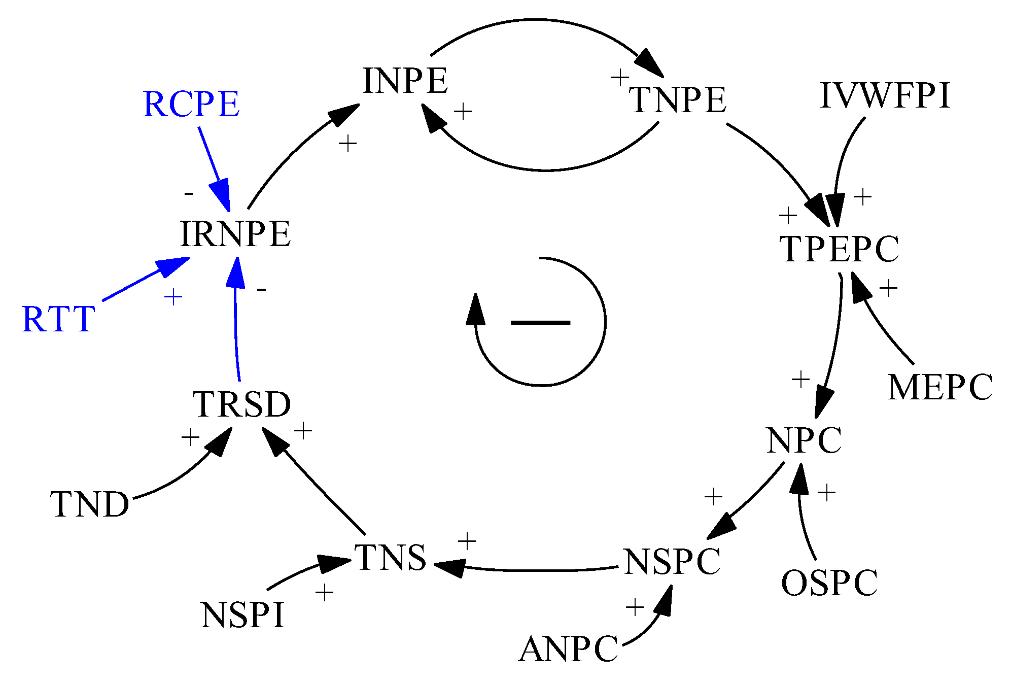
Firstly, at a practical level, the increasing rate of national pension expenditure (INPE) directly determines the state variable of total national pension expenditure (TNPE) for the current year’s pension supply subsystem, thus directly determining the supply capacity of pension institutions and pension communities. At the level of the mathematical model, the INPE should be related to the output variable of the total ratio between supply and demand (TRSD). When the TRSD is low, relevant policies should be formulated to increase the next year’s INPE. When the TRSD reaches the expectation, relevant policies should be relaxed or tightened to budget the next year’s INPE. Therefore, under the background of China’s pension policy changes in 2019, the next year’s INPE should be related to the TRSD. In addition, two parameter variables, Regulation Threshold of Total Ratio between Supply and Demand (RTT) and Regulation Coefficient of Pension Expenditure (RCPE), are added to the model. The optimized causality diagram of this part is shown in Figure 1.

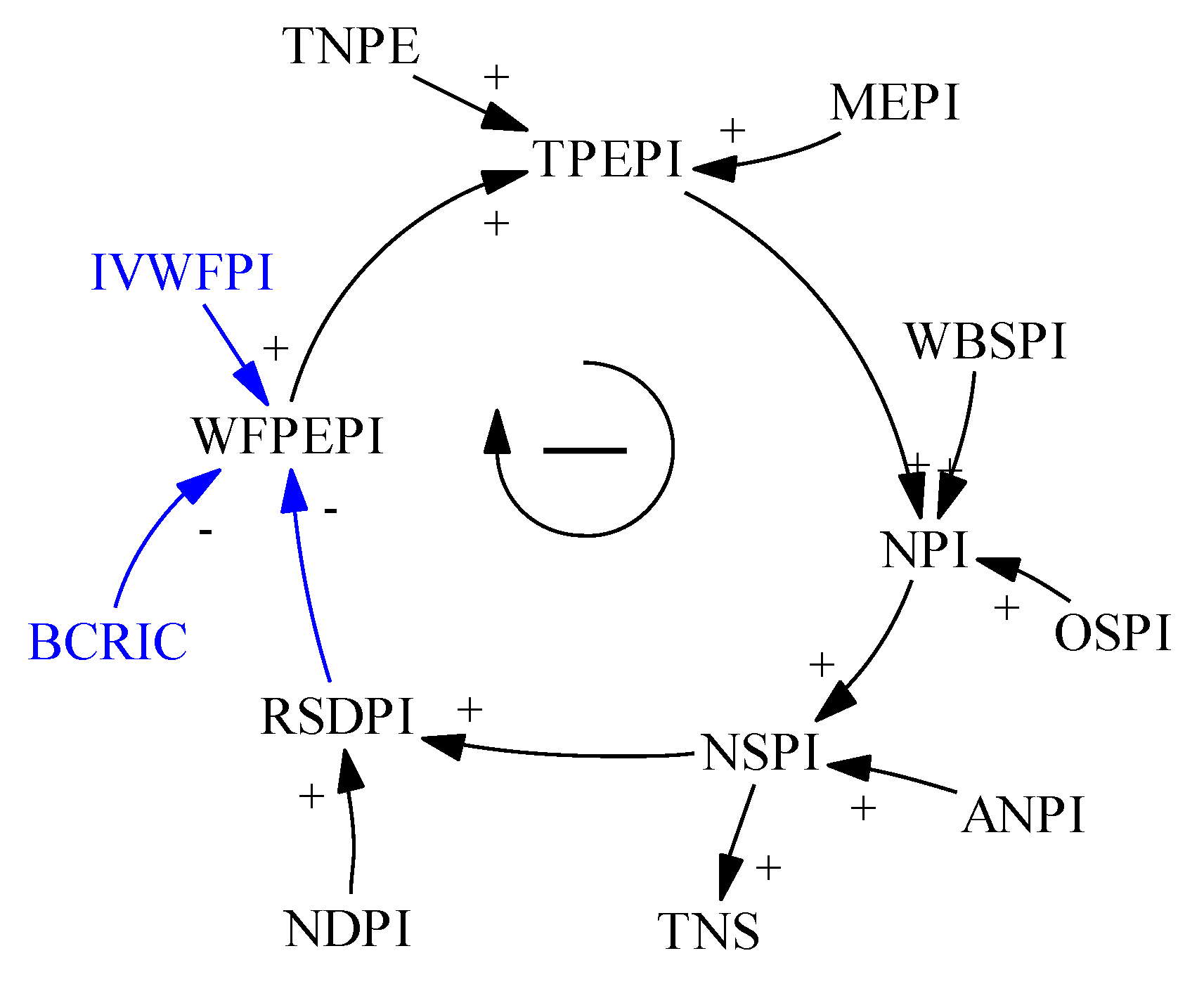
Secondly, from 2015 to 2020, the central government allocated RMB 5 billion (approximately USD 743 million) to encourage new pilot programs of home-based elderly care services to be provided by communities in 203 cities. [34] A large number of community aged service centers were built and put into use in 2020, which has greatly improved the supply of aged services. Therefore, the state’s financial expenditure ratio of pension institutions and pension communities should change with the national policy. It is necessary to establish a relationship between the weight factor of pension expenditure for pension institutions (WFPEPI) and the ratio between the supply and demand of pension institutions (RSDPI) or establish a relationship between the weight factor of pension expenditure for pension communities (WFPEPC) and the ratio between the supply and demand of pension communities (RSDPC). When the RSDPI is imbalanced, the WFPEPI in the next year should be dynamically increased or decreased to improve the supply–demand situation. Thus, this part of the model is improved. In addition, the initial value of the weight factor of institutional pension expenditure (IVWFPI) and the balance coefficient of the supply and demand ratio of institutional community pension (BCRIC) were added. The optimized causality diagram of this part is shown in Figure 2.

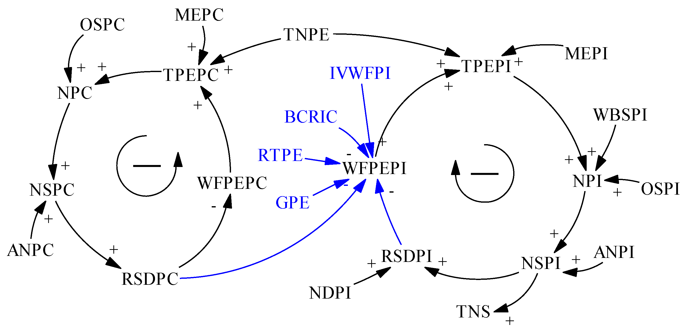
Thirdly, both pension communities and pension institutions are indispensable parts of the aged service system, and the balanced development of the two can further improve the TRSD. Therefore, it is necessary to correlate the difference between the RSDPI and the RSDPC with the WFPEPI or the WFPEPC. When the difference between the RSDPI and the RSDPC is positive, relevant policies should be formulated to adjust the WFPEPI. In addition, with a reduction in the difference, relevant policies should be maintained or tightened to reduce the adjustment range of the WFPEPI, so that the aged service resources allocation of pension institutions and pension communities is more reasonable and holds a stronger self-regulation ability. Thus, this part of the model is improved. In addition, two parameter variables, the community pension expenditure weight regulation threshold (RTPE) and the community pension expenditure weight regulation amplification coefficient (GPE), were added. The optimized causality diagram of this part is shown in Figure 3.

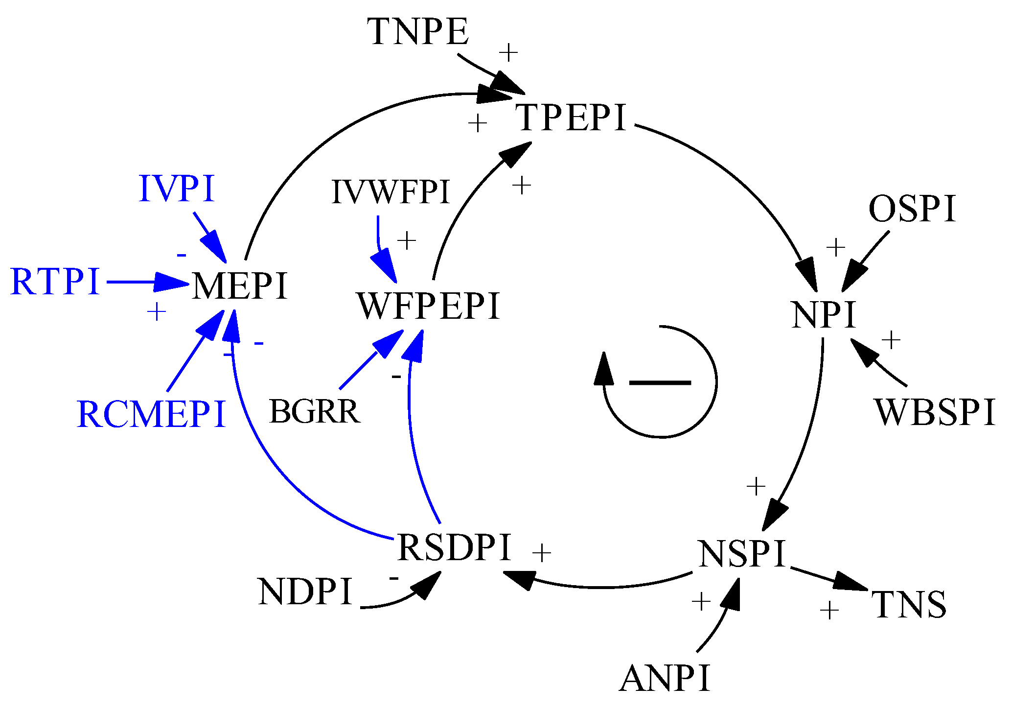
Fourthly, the market engagement represents the marketization level of elderly care services. The higher the market engagement is, the more social investment, so the market engagement should be related to the demand of the existing market. When the market demand is large, the enthusiasm for market engagement is high. On the contrary, the enthusiasm for market engagement will gradually decrease if the market demand is small. At present, most pension institutions are still run by the government. According to the statistics released by the National Office for Ageing, the proportion of pension institutions run by social forces in China reached 41.5% in 2015, and it is expected to reach 50% in 2020 [35]. The average participation rate of pension institution market from 2015 to 2019 was 0.45. However, the pension communities mainly rely on the communities and streets to provide elderly care services, with little market engagement. The average participation of the pension community market from 2015 to 2019 was 0.1. Relevant policies such as “City-Enterprise Linkage, Inclusive Pension” issued in 2019 have stimulated market capital participation, which is reflected in the mathematical model. Constant market engagement is not conducive to the self-regulation of system output. Therefore, the market engagement should be related to the ratio between supply and demand. When the ratio between supply and demand deviates greatly from the expected value, relevant policies should be formulated to increase the pension market engagement so as to reduce the deviation. On the contrary, when the ratio between supply and demand approaches or exceeds the expected value, relevant policies should be maintained or tightened to promote the pension market engagement to stabilize or decrease. Thus, this part of the model is improved. The institutional pension market participation MEPI is changed from a parameter variable to an auxiliary variable. In addition, three parameter variables, the initial value of market engagement of pension institutions (IVPI), the regulation threshold of market engagement of pension institutions (RTPI), and the regulation coefficient of market engagement of pension institution (RCMEPI) are added. The optimized causality diagram of this part is shown in Figure 4.

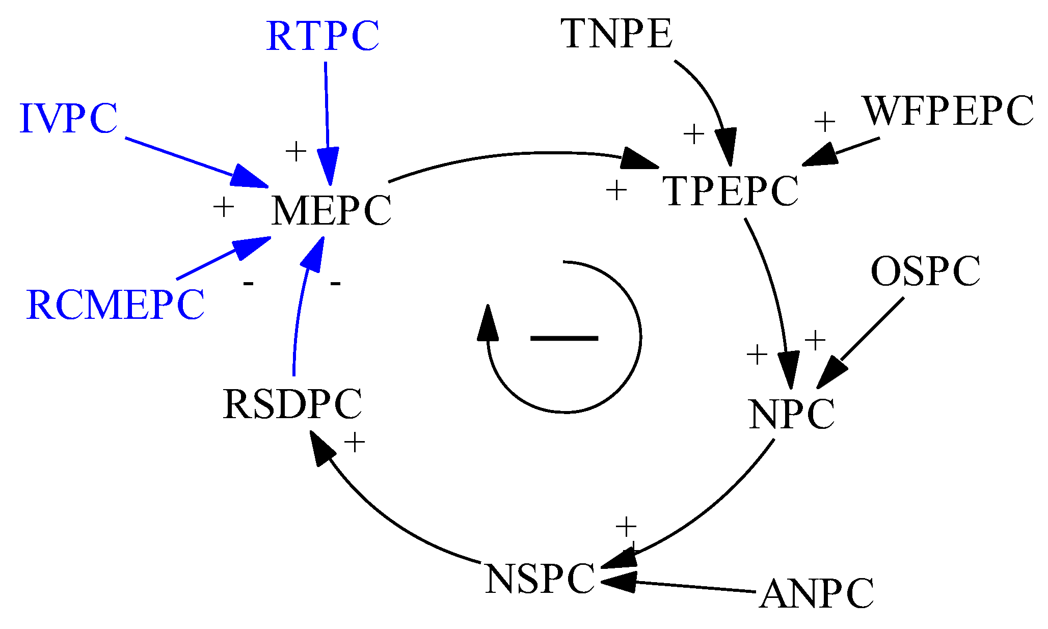
For community endowment resources supply and demand, three parameter variables are added: the initial value of market engagement of pension communities (IVPC), the regulatory threshold of market engagement of pension communities (RTPC), and the regulatory coefficient of market engagement of pension communities (RCMEPC). The optimized causality diagram of this part is shown in Figure 5.

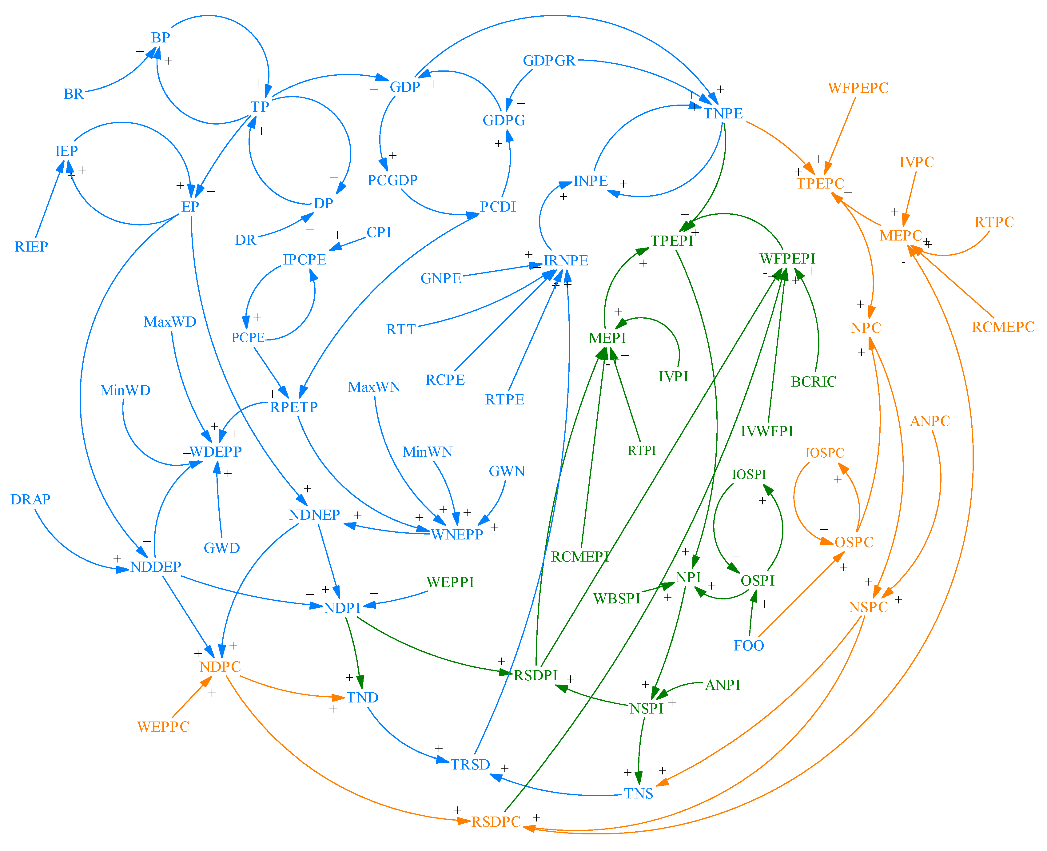
Combined with the above analysis, the next steps are to further refine the variables in the above subsystems, sort out the variables contained in the system, and show the changes of causality after configuration optimization in blue (the black part is the content completed by the author’s previous research [31]), to form the causality diagram for the supply and demand system of aged service resources, as shown in Figure 6.

3. Materials and Methods

Among many sensitivity analysis methods, trajectory sensitivity analysis and matrix sensitivity analysis can analyze the parameter sensitivity of the mathematical model based on the system state equations. According to the literature research, although the accuracy of the first-order trajectory sensitivity is higher than that of the first-order matrix sensitivity, the common problem of the first-order sensitivity analysis is that the variation range of system parameters should not be too large, and the sensitivity analysis results will have a large deviation when the variation range of system parameters change by more than 5%. There are many parameters in the supply and demand system of aged service resources and the variation range of many parameters is greater than 5% in actual situations, so it is necessary to apply the second-order sensitivity analysis method for the higher accuracy. Since the equation of the second trajectory sensitivity analysis method is very complex, while the speed of computer operation is slow, it is only suitable for the case of few parameters and uncomplicated system model. The second-order matrix sensitivity analysis method holds a faster calculation speed without losing the accuracy of solution, which is suitable for the case of more system parameters and can be used in this paper.

However, the existing theoretical models can only solve the influence degree of each parameter on the state variables of the system. The supply and demand system of aged service resources established in this paper has complex output equations, and the existing theoretical model needs to be extended before sensitivity analysis, so that it can be applied to the parameter sensitivity analysis for the supply and demand system of aged service resources.

The general expression of the state space of the system is

$$\left\{\begin{array}{l}\dot{x}=Ax+Bu=f(x,u,\alpha ,t)\\ y=Cx+Du\end{array}\right.$$

(1)

where, A is the $m\times m$ order parameter matrix, B is the $m\times p$ order parameter matrix, C is the $q\times m$ order parameter matrix, D is the $q\times p$ order parameter matrix, $x$ is the $m$ dimension state variable, $u$ is the $p$ dimension input variable, $\alpha$ is the r dimension parameter variable, y is the $q$ dimension output variable, and t represents time.

The mathematical model of high-order system can be expressed as:

$$g(x,u,\alpha ,t)=0$$

(2)

In Equation (2), the state variable $x$, the input variable $u$, $\alpha$, and the time $t$ are the same as those defined in Equation (1).

Equation (2) is an equation group of $\mathrm{m}$ order ($\mathrm{m}$ represents the number of state variables). Through the system state Equation (1), it can be calculated that when the input variable $u_0$ and parameter variable ${\alpha }_0$ are constant, the initial value of Equation (2) is:

$$g(x_0,u_0,{\alpha }_0,t)=0$$

(3)

In Equation (3), the variation $\Delta \alpha$ of parameter variable $\alpha$ and the variation $\Delta u$ of input variable $u$ will cause the variation $\Delta x$ of state variable $x$, namely:

$$g(x_0+\Delta x,u_0+\Delta u,{\alpha }_0+\Delta \alpha ,t)=0$$

(4)

Equation (4) is expanded by first-order Taylor, which can be converted into:

$$g(x_0+\Delta x,u_0+\Delta u,{\alpha }_0+\Delta \alpha ,t)\approx g(x_0,u_0,{\alpha }_0,t)+g_x·\Delta x+g_u·\Delta u+g_{\alpha }·\Delta \alpha$$

(5)

Substituting Equation (3) into Equation (5) to obtain:

$$g_x·\Delta x+g_u·\Delta u+g_{\alpha }·\Delta \alpha =0$$

(6)

Equation (6) can be converted into the following form:

$$\Delta x=-g_x{}^{-1}·g_u·\Delta u-g_x{}^{-1}·g_{\alpha }·\Delta \alpha$$

(7)

where $g_x$ is the Jacobian matrix $\partial g/\partial x$, $g_{\alpha }$ is the Jacobian matrix $\partial g/\partial \alpha$, and $g_u$ is the Jacobian matrix $\partial g/\partial u$.

In the mathematical model of aged service resources allocation, because the input variable is time, it is considered that $\Delta u=0$. Therefore, this paper only pays attention to the parameter sensitivity of each parameter variable. Assume that $S_{\alpha }$ is the $n\times p$ order matrix:

$$S_{\alpha }=g_x{}^{-1}·g_{\alpha }$$

(8)

Substituting Equation (8) into Equation (7), without considering the influence of input variables where $\Delta u=0$, can obtain:

$$\Delta x=-S_{\alpha }·\Delta \alpha$$

(9)

Equation (9) is the first-order matrix sensitivity equation, where $S_{\alpha }$ represents the $m\times p$ order sensitivity matrix of parameter variable $\alpha$.

The second-order Taylor expansion of Equation (4) is carried out and $\Delta u=0$ is brought into it, which can be converted into:

$$\begin{array}{c}\hfill g(x_0+\Delta x,u_0,{\alpha }_0+\Delta \alpha ,t)\approx g(x_0,u_0,{\alpha }_0,t)+g_x·\Delta x+g_{\alpha }·\Delta \alpha +\frac{1}{2}\Delta x^{\mathrm{T}}·g_{xx}·\Delta x\\ \hfill +\frac{1}{2}\Delta x^{\mathrm{T}}·g_{x\alpha }·\Delta \alpha ++\frac{1}{2}\Delta {\alpha }^{\mathrm{T}}·g_{\alpha x}·\Delta x+\frac{1}{2}\Delta {\alpha }^{\mathrm{T}}·g_{\alpha \alpha }·\Delta \alpha \end{array}$$

(10)

Equation (10) is the general expression of second-order matrix sensitivity equation, which is the three-dimensional matrix equation. When only studying the influence for the variation $\Delta {\alpha }_i$ of a certain parameter variable ${\alpha }_i$ on a state variable $x_j$, the variation $\Delta \mathbf{\alpha }$ of the parameter variable $\mathbf{\alpha }$ changes from the $p\times 1$ order two-dimensional matrix to the first-order one-dimensional matrix, and the variation $\Delta \mathit{x}$ of the parameter variable $\mathit{x}$ changes from the $n\times 1$ order two-dimensional matrix to the first-order one-dimensional matrix. All three-dimensional matrixes can be simplified into the first-order one-dimensional matrix, that is, the complex matrix operations are simplified into one-dimensional algebraic equations one by one. Taking the three-dimensional matrix $g_{x\alpha }$ as an example, the matrix is changed from $n\times n\times p$ order to first-order one-dimensional matrix $g_{x_j{\alpha }_i}^j$ [36]. Modified Equation (10) can be expressed as:

$$g(x_{j0},u_0,a_{i0},t)+g_{x_j}^j·\Delta x_j+g_{{\alpha }_i}^j·\Delta a_i+\frac{1}{2}\Delta x_j{}^2·g_{x_j{x}_j}^j+\Delta x_j·\Delta a_i·g_{x_j{\alpha }_i}^j+\frac{1}{2}\Delta {\alpha }_{{}_i}^2·g_{{\alpha }_i{\alpha }_i}^j=0$$

(11)

Equation (11) is transformed into the sensitivity equation of unary quadratic matrix with independent variable $\Delta {\alpha }_i$ and dependent variable $\Delta x_j$, namely:

$$\frac{1}{2}{g}_{x_j{x}_j}^j·\Delta x_j{}^2+\left(g_{x_j}^j+\Delta {\alpha }_i·g_{x_j{\alpha }_i}^j\right)\Delta x_j+\frac{1}{2}\Delta {\alpha }_{{}_i}^2·g_{{\alpha }_i{\alpha }_i}^j+g_{{\alpha }_i}^j·\Delta a_i+g(x_{j0},u_0,a_{i0},t)=0$$

(12)

The above equation is called the simplified expression of second-order matrix sensitivity equation, and the second-order matrix sensitivity of the variation $\Delta {\alpha }_i$ of state variable $x_j$ to parameter variable ${\alpha }_i$ can be obtained only by solving a univariate quadratic equation with time-varying coefficients.

It can be seen from Equation (12) that the traditional second-order matrix sensitivity theory can only study the influence degree of system parameter variables on state variables [36]. While in the system state space expression, the state equation and the output equation are inseparable, and the optimized mathematical model of aged service resources allocation established in this paper has a complex output equation. This section extends the traditional second-order matrix sensitivity theory and makes its application range extend from the state equation to the whole state space.

When the output equation of the system is as follows:

$$y=f(x,u,\alpha ,t)$$

(13)

The variation of the parameter variable can cause the change of the state variable. Under the combined action, the output variable of the system will also change. Equation (13) can be changed into the following form:

$$y_0+\mathsf{\Delta }y=f(x_0+\mathsf{\Delta }x,u_0+\mathsf{\Delta }u,{\alpha }_0+\mathsf{\Delta }\alpha ,t)$$

(14)

If the right side of the equal sign of Equation (14) is expanded by the first-order Taylor, the variation of the output variable can be expressed as:

$$\Delta y=f(x_0,u_0,{\alpha }_0,t)+f_x·\Delta x+f_u·\Delta u+f_{\alpha }·\Delta \alpha -y_0$$

(15)

where $f_x$ is the $q\times m$ order matrix, $f_u$ is the $q\times p$ order matrix, and the $f_{\alpha }$ is the $q\times r$ order matrix. In Equation (15):

$$f(x_0,u_0,{\alpha }_0,t)=y_0$$

(16)

Substituting Equation (16) into Equation (15) with $\Delta u=0$, the equation can be simplified as follows:

$$\Delta y=f_x·\Delta x+f_{\alpha }·\Delta \alpha$$

(17)

By combining Equations (12) and (17), the sensitivity of the second-order matrix can be extended to the whole state space. Among them, $\Delta x$ can be obtained from Equation (12) after $\mathrm{m}\times \mathrm{r}$ times of repeated calculations, and the second-order matrix sensitivity of output variable $y$ to parameter variable $\alpha$ can be obtained by bringing the results into Equation (17).

In order to evaluate the sensitivity results of each parameter more intuitively and quantitatively, this section defines two different sensitivity indexes.

(1)

Sensitivity index 1

The maximum absolute value for the influence of each parameter change on the output variable is defined as sensitivity index 1, which is used to represent the maximum influence of the parameter changes on the output variables. The specific equation of sensitivity index 1 is:

$$S_1={\left|f_x·\Delta x+f_{\alpha }·\Delta \alpha \right|}_{max}$$

(18)

where $S_1$ is the sensitivity index 1.

(2)

Sensitivity index 2

The average value for the influence of each parameter change on the output variable is defined as sensitivity index 2, which is used to characterize the average influence of the parameter changes on the output variables. The specific equation of sensitivity index 2 is:

$$S_2=\frac{{\displaystyle {\int }_{t_1}^{t_2}\left(f_x·\Delta x+f_{\alpha }·\Delta \alpha \right)}\mathrm{d}t}{t_2-t_1+1}$$

(19)

where $S_2$ is the sensitivity index 2, $t_1$ is the starting time (year), and $t_2$ is the ending time (year).

By analyzing the above two sensitivity indexes of each parameter, the influence degree of each parameter change on the output variables can be quantified more clearly and effectively. In the quantitative sensitivity analysis, each parameter will be analyzed for the mathematical model before and after optimization, so as to intuitively compare the quantitative sensitivity of each parameter under the same mathematical model.

4. Result

4.1. Simulation Analysis

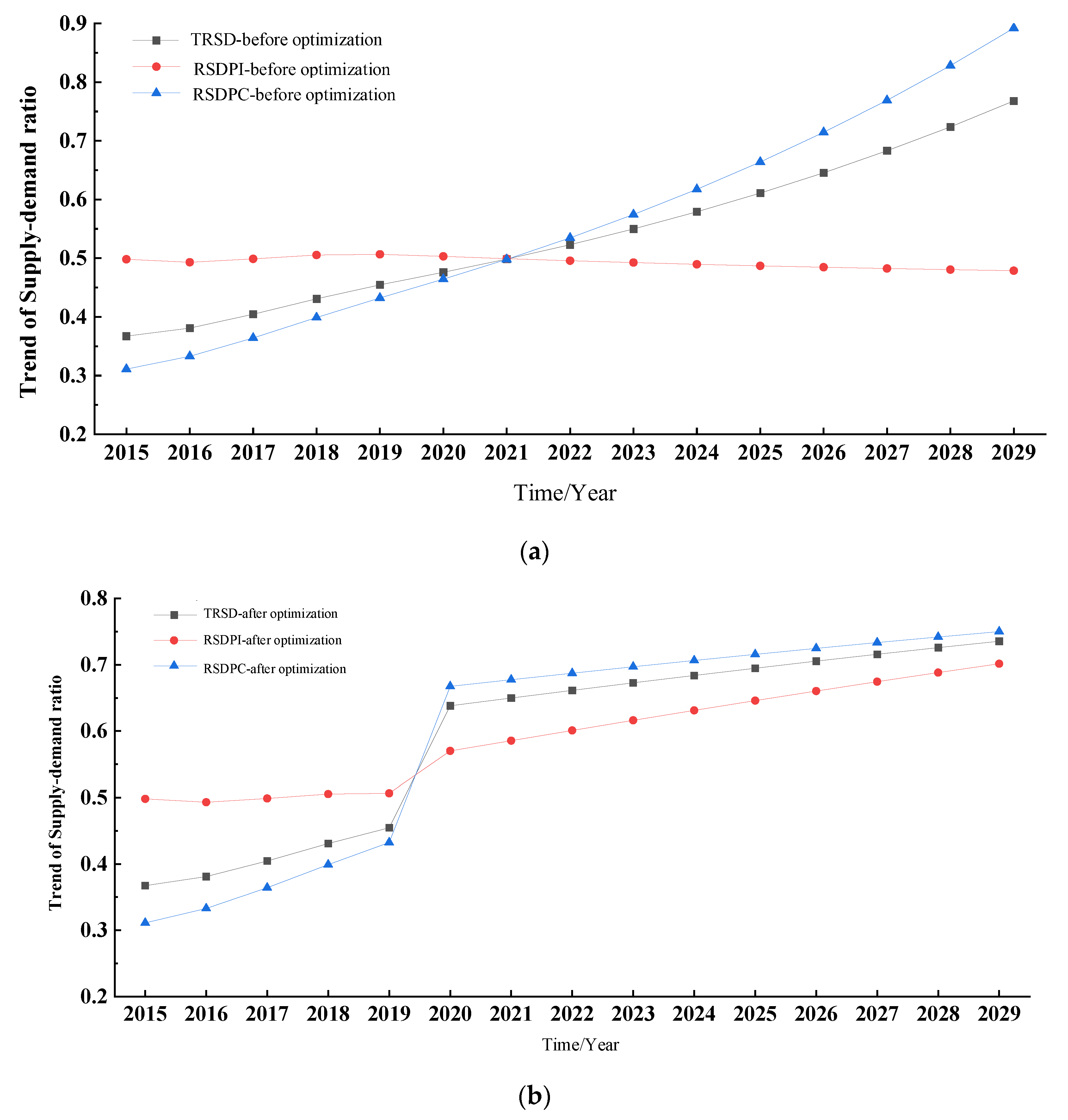
According to the four model optimization measures proposed in Section 2, MATLAB/Simulink software was used for simulation. The trend of three output variables of the optimized model was obtained. To clearly show the differences of the three variables involved in the output variables before and after the optimization of the mathematical model, the simulation values are shown in Figure 7.

It can be concluded from Figure 7 that the TRSD and RSDPC both increased year by year with time, and the growth rate did not slow down, because the mathematical model before optimization lacked correlation with variables such as the TRSD, pension market engagement, the IRNPE, weight factors of pension institutions and communities, etc., which is obviously inconsistent with the actual situation. After the optimization of the mathematical model, the supply and demand situation of elderly care services in China significantly improved in 2020, with TRSD, RSDPI, and RSDPC increasing from 0.45, 0.51, and 0.43 to 0.64, 0.57, and 0.67, respectively, with annual growth rates of 43.2%, 11.8%, and 55.8%, respectively. After 2020, the supply and demand situation of elderly care services in China has further improved. By 2029, TRSD, RSDPI, and RSDPC will have increased to 0.74, 0.70, and 0.75, respectively, with an increase of 15.6%, 22.8%, and 11.9%, respectively, compared with 2020. It can be seen from the above data that after 2020, the supply and demand situation of aged service in China has further improved, and the growth trend of RSDPC has obviously slowed down, after a substantial increase in 2020. It is predicted that the gap between RSDPC and RSDPI will gradually narrow, and, with the development of time, the supply and demand situation of elderly care services in China will gradually become stable, which also shows the rationality and correctness of the measures for joint optimization of pension institutions and communities.

4.2. Dynamic Analysis of Parameter Sensitivity in Supply and Demand System of Aged Service Resources

Before the parameter sensitivity analysis in this section, the parameters need to be classified. There are 31 parameter variables in the system. Among them, 18 parameters that did not change from 2015 to 2029 were selected as parameter sensitivity analysis, and the variation of each parameter sensitivity before and after the optimization of resource allocation measures can be seen. The above parameters are shown in

Table 1. The 18 parameter variables and numbers.

No.	Parameter Variables	No.	Parameter Variables	No.	Parameter Variables
1	Factor of Per Capita Disposable Income (FPCDI)	7	Weight Factor of Pension Expenditure for Pension Institutions (WFPEPI)	13	Maximum Values of WDAPP (MaxWD)
2	Average of CPI (ACPI)	8	Market Engagement of Pension Community (MEPC)	14	Minimum Values of WDAPP (MinWD)
3	Disability Rate of Aging Population (DRAP)	9	Willingness of Aging Population to participate in Pension Institutions (WAPPI)	15	Maximum Values of WNAPP (MaxWN)
4	Rate of Increase in Aging Population (RIAP)	10	Weight factor of Beds’ construction Subsidies of Pension Institutions (WBSPI)	16	Minimum Values of WNAPP (MinWN)
5	Factor of OSPI and OSPC (FOO)	11	Average Numbers of beds in Pension Institutions (ANPI)	17	GWD $K_{A1}$
6	Market Engagement of Pension Institutions (MEPI)	12	Average Amount of aging population served by Pension Communities (ANPC)	18	GWN $K_{A2}$

.

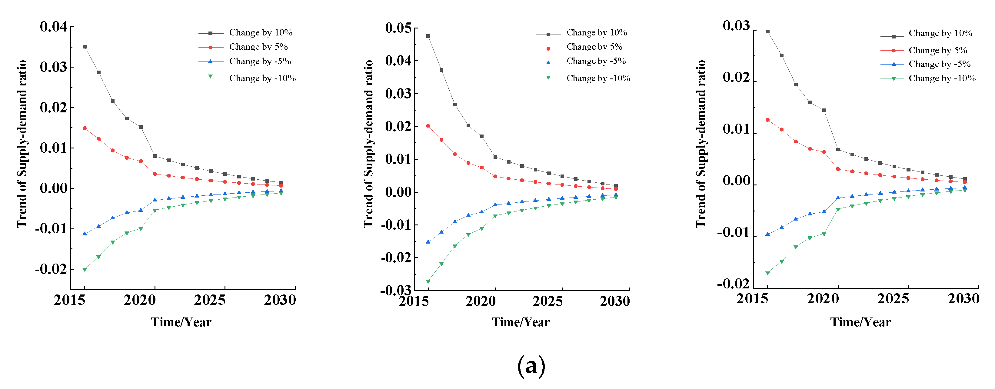
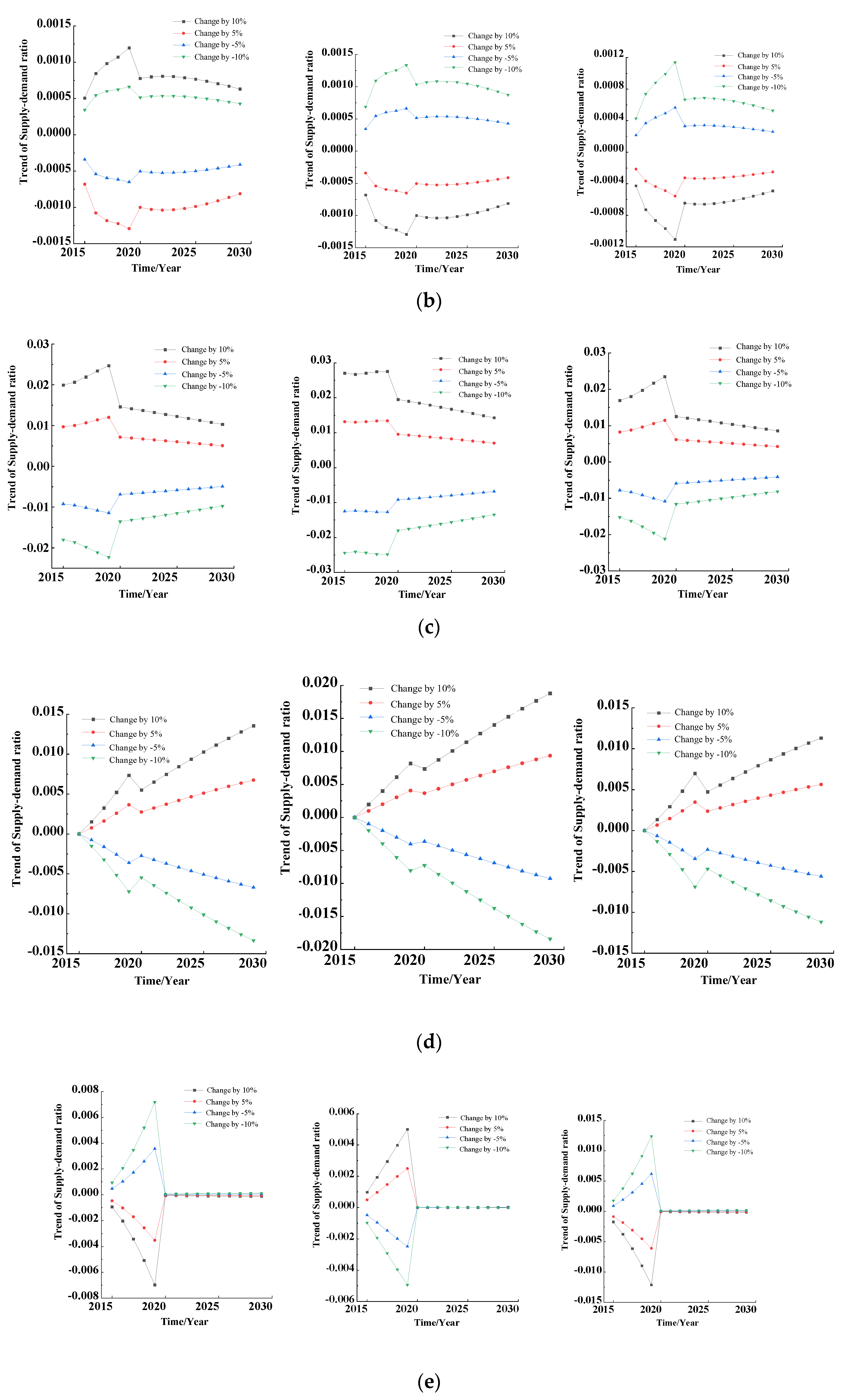
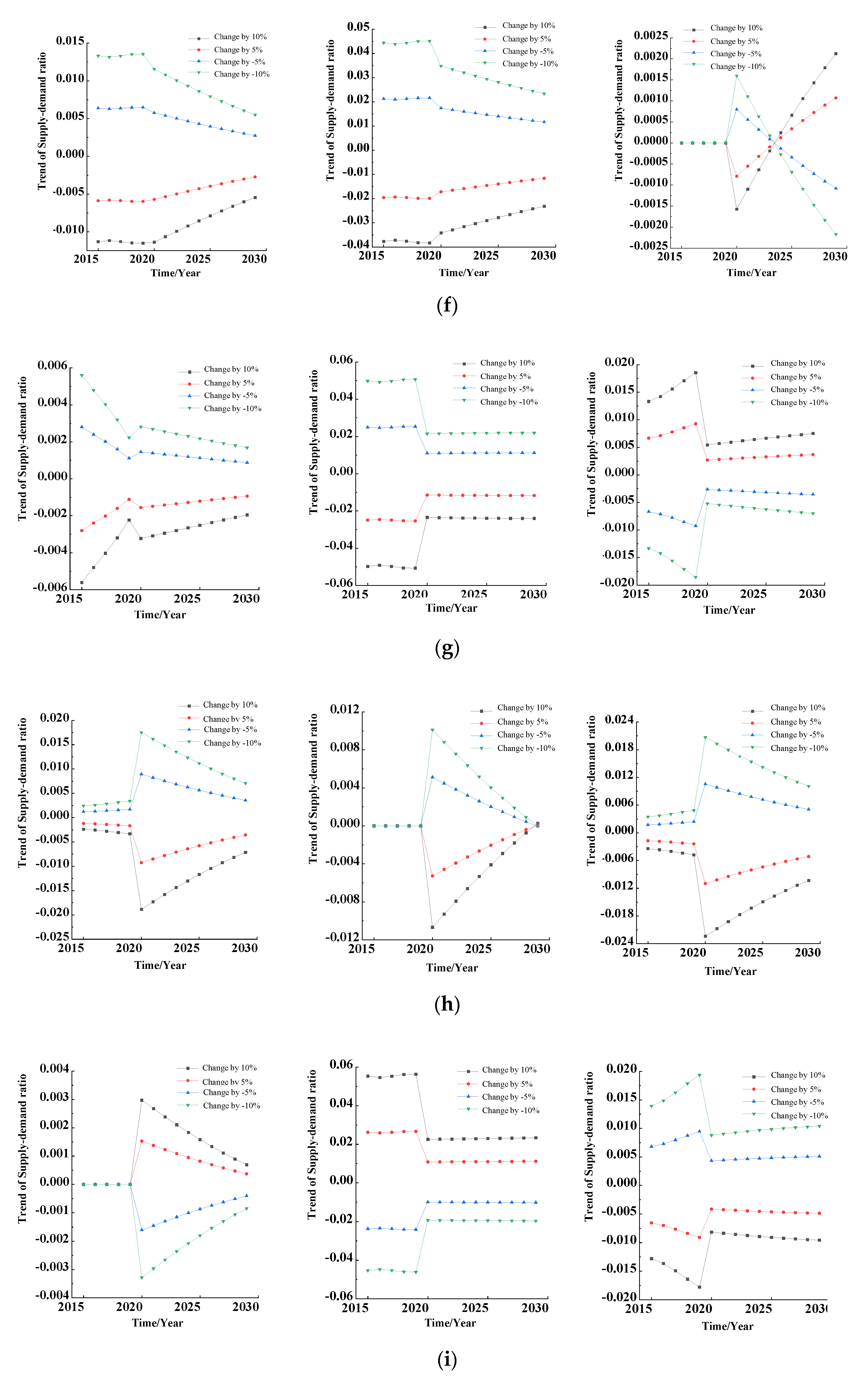
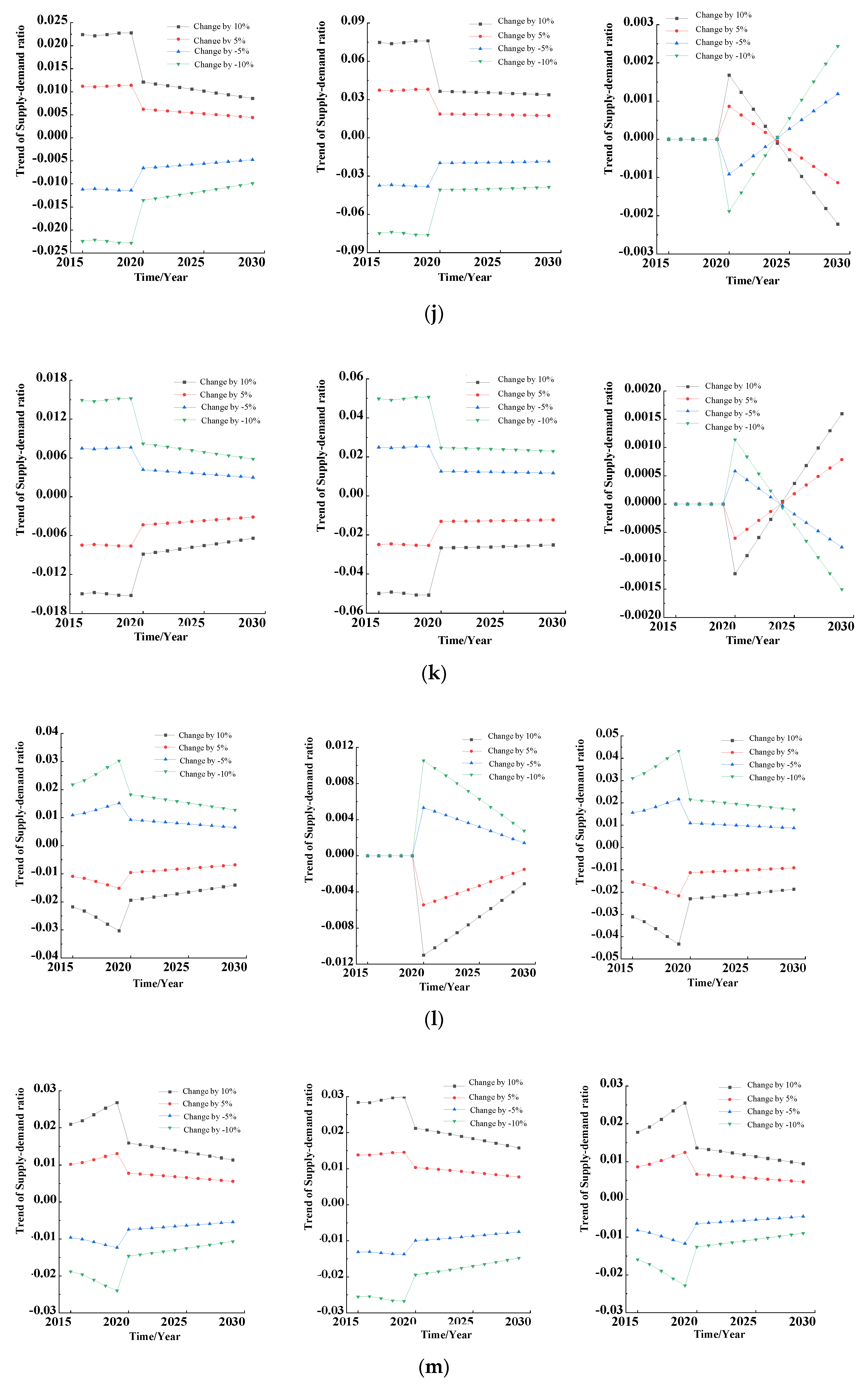
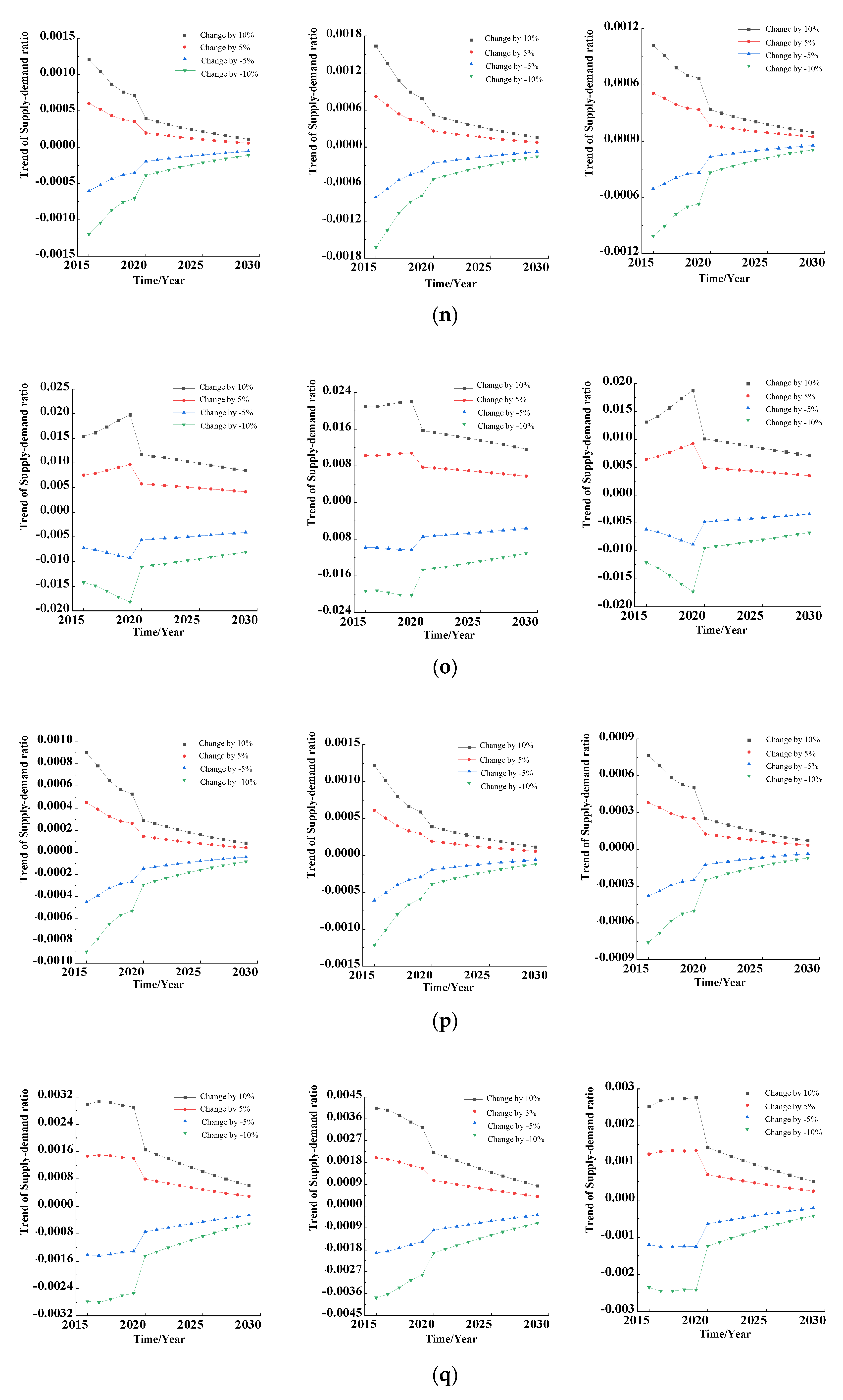
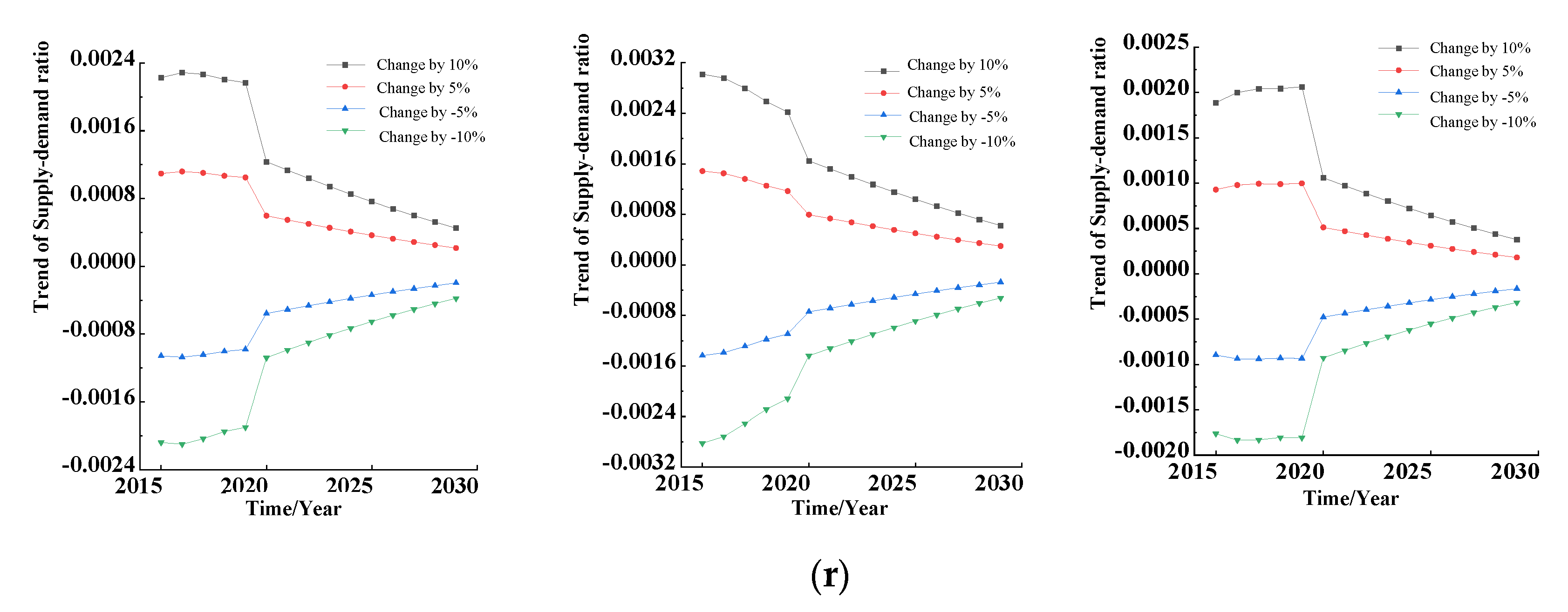
In this section, the influence degree on the output variables when the parameters change by −10%, −5%, 5%, and 10% in different years is studied. The above influence degree can be programmed and calculated by MATLAB software, according to Equation (17). A comparison of dynamic sensitivity of parameters is shown in Figure 8. The dynamic sensitivity results of parameters to output variables such as TRSD, RSDPI, and RSDPC are shown from left to right in each figure.

As can be seen from Figure 8, different variations of each parameter have a different influence on the three output variables, and, after the optimization of the mathematical model, the influences of the dynamic sensitivity curves of most parameters on the three output variables decrease with time, which shows that the robustness of the system is improved, and the sensitivity to parameter perturbation is reduced.

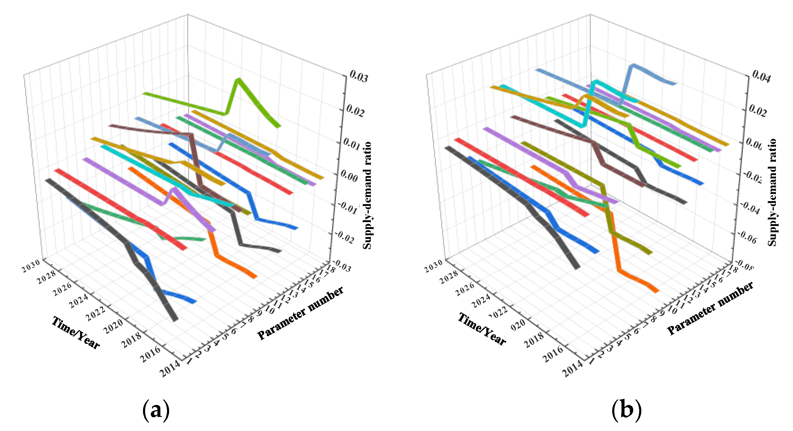
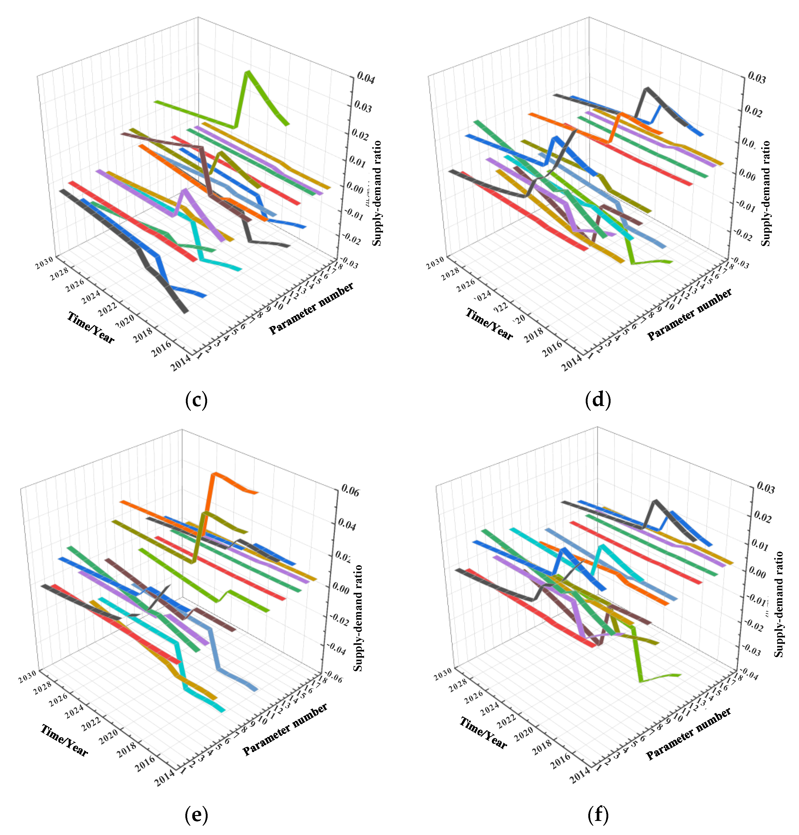
In order to intuitively see the influence degree of different parameter changes on the three output variables, the dynamic sensitivity curves of 18 parameters are integrated, and a three-dimensional comparison diagram of dynamic sensitivity is formed, as shown in Figure 9.

It can be seen from Figure 9 that although some parameters have similar dynamic sensitivity variation rules, their specific values are not the same; in addition, the increase in some parameters will lead to the increase in output variables, while the increase in some parameters will lead to the decrease in output variables. The sensitivity of each parameter will be quantitatively analyzed in view of the above phenomena.

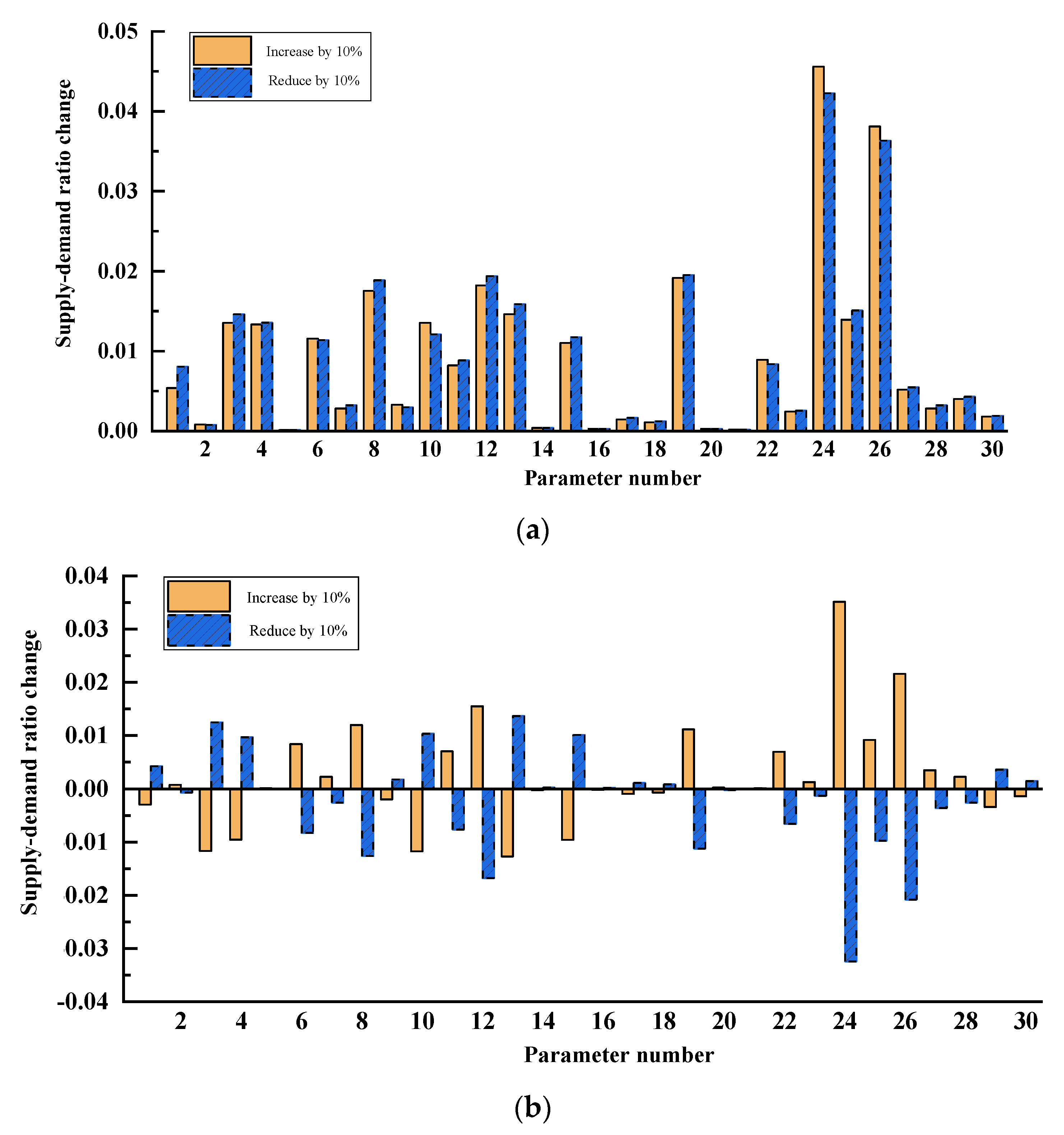
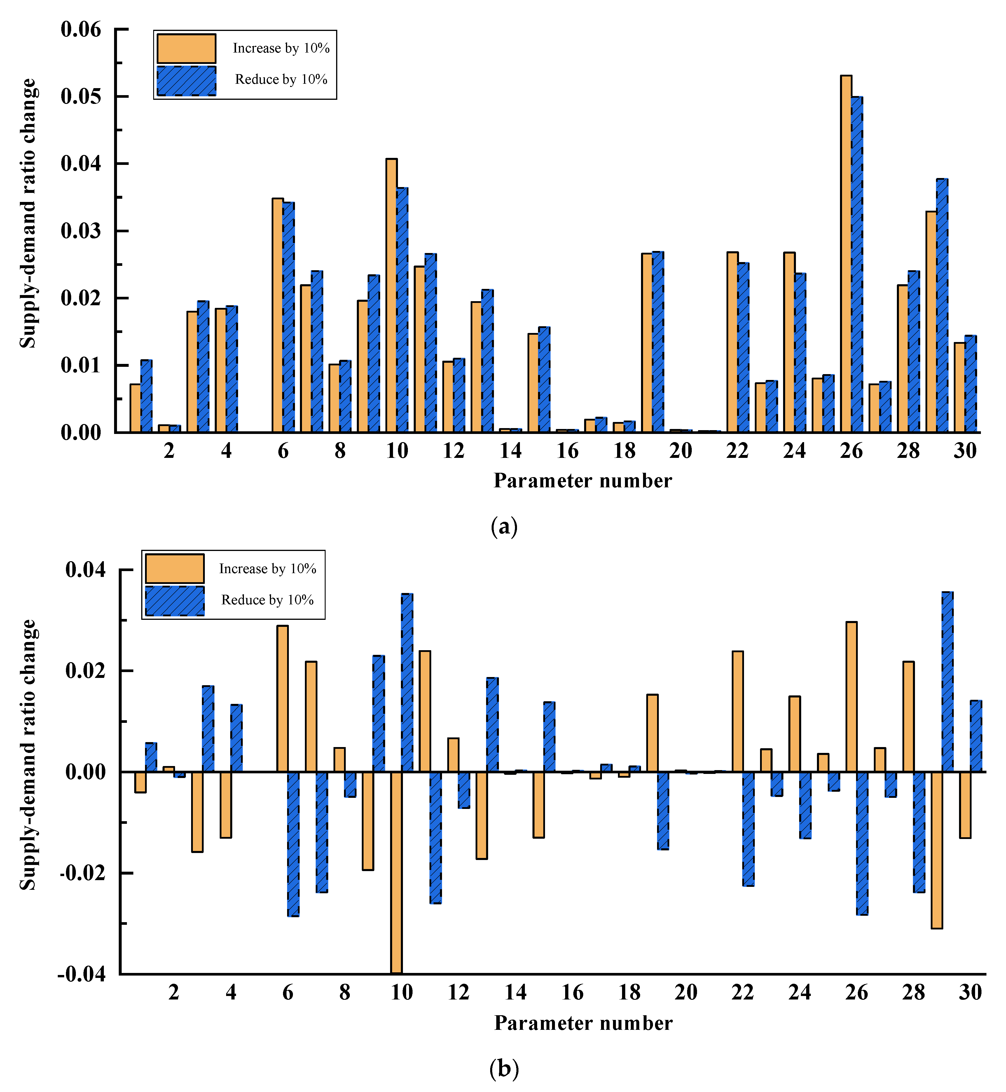
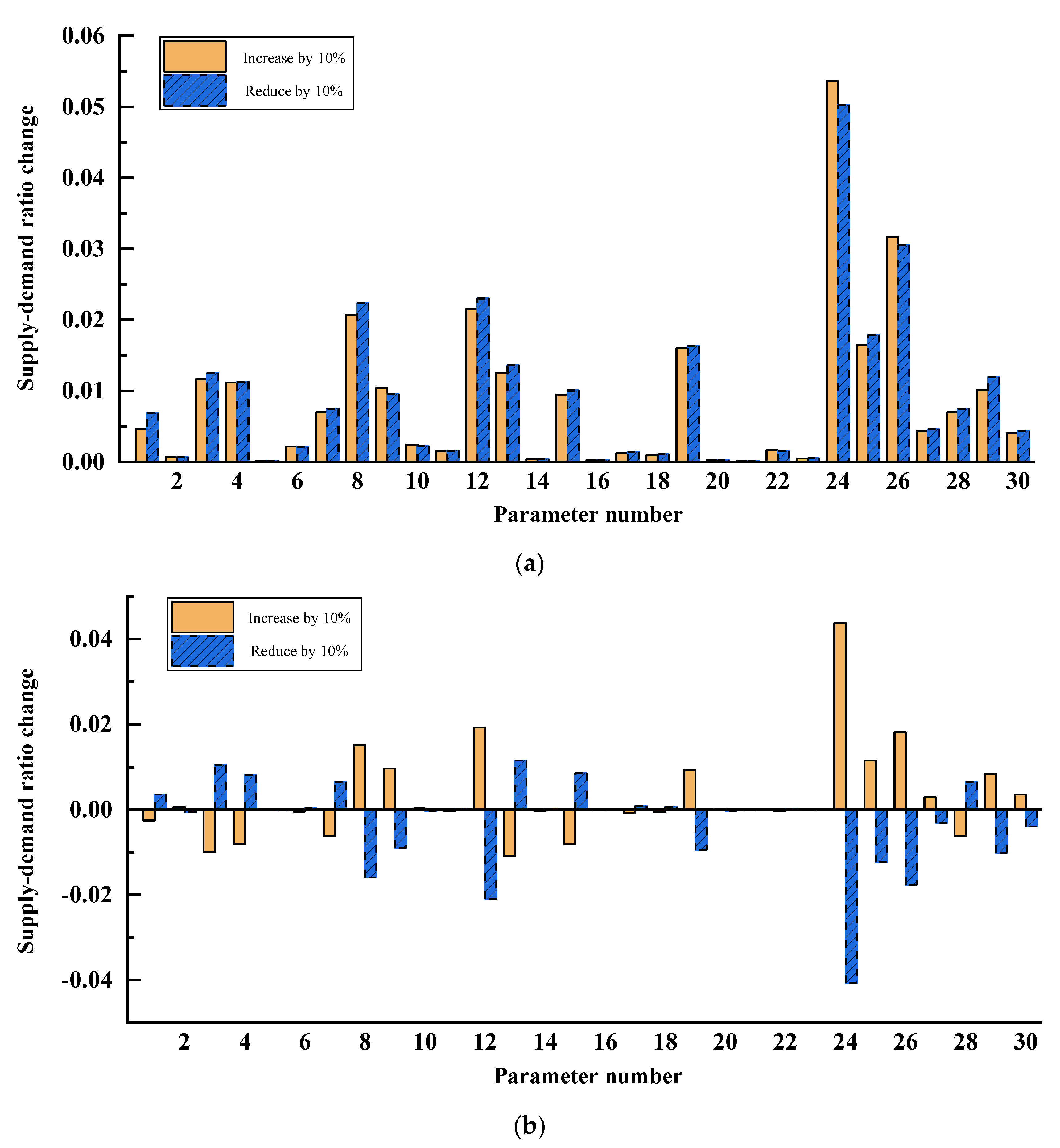
All 30 parameters in the mathematical model shown in Equation (1) will be analyzed (since WFPEPI and WFPEPC are interrelated and add up to 1, only the parameter WFPEPI is studied). The analysis results are shown in Figure 10, Figure 11 and Figure 12 in which parameters 1 to 18 correspond to Table 1, and parameters 19 to 30 correspond to

Table 2. The remaining 12 parameter variables in the model, except Table 6.

No.	Parameter Variables	No.	Parameter Variables	No.	Parameter Variables
19	GDPGR	23	Regulation Coefficient of Market Engagement of Pension Institution (GMEPI)	27	Regulation Coefficient of Pension Expenditure (GNPE)
20	BR	24	Regulation Threshold of Market Engagement of Pension Communities (RTPC)	28	Balance Coefficient of Pension Community Supply and Demand Ratio (BGRR)
21	DR	25	Regulation Coefficient of Market Engagement of Pension Institution (GMEPC)	29	Regulation Threshold of Weight of Pension Expenditure in Communities (RTPE)
22	Regulation Threshold of Market Engagement of Pension institutions (RTPI)	26	Regulation Threshold of Total Ratio between Supply and Demand (RTT)	30	Gain of Weight Regulation of Pension Expenditure (GPE)

.

From Figure 10, Figure 11 and Figure 12, it can be seen that the influence for 10% change of each parameter on the three output variables presents different laws. As parameter 22 to parameter 30 are new parameter variables in the optimized mathematical model, they are all thresholds or amplification coefficients of the closed loop built in the mathematical model. The sensitivity dynamic and quantitative results will be combined for discussion.

5. Discussion

According to the results of the dynamic sensitivity of the parameters, the following rule can be summarized, where parameter x represents the x-th parameter in Table A1 in Appendix A:

Firstly, parameter 1, parameter 14, and parameter 16 have the same variation rules. Their dynamic sensitivity curves converge and decrease gradually with time, and their influence laws on the three output variables are similar.

Secondly, parameter 2, parameter 3, parameter 13, parameter 15, parameter 17, and parameter 18 have the same variation rules. Their dynamic sensitivity curves changed greatly around 2020. Before 2020, their dynamic sensitivity curves increased slowly or remained stable with time, then decreased sharply in 2020, and gradually converged and decreased with the change of time. Their influences on the three output variables were similar.

Thirdly, parameter 6, parameter 10, and parameter 11 have the same variation rules. Their dynamic sensitivity curves for the output variable TRSD and the output variable RSDPI are the same as those summarized in the second point above, except that they have different dynamic sensitivity curves for the output variable RSDPC. The reason for the above phenomenon is that the above three parameters are all directly related to pension institutions in the supply subsystem of aged service resources. Before the model optimization, pension institutions and pension communities were not directly related, so the changes of the above three parameters will have no impact on RSDPC before 2020. After 2020, due to the optimization of mathematical models, their changes have a similar influence on RSDPC.

Fourthly, for parameter 4, parameter 5, parameter 7, parameter 8, parameter 9, and parameter 12, the variation rules of these six parameters are different from the other parameters, so they need to be discussed separately. The dynamic sensitivity curve of parameter 4 gradually increases with time, and the influence laws on the three output variables are similar. This is because the amount of the elderly population (EP) is a state variable, while the rate of increase in elderly population (RIAP) changes exponentially with time, so the longer the amount of time is, the more significant the influence. The dynamic sensitivity curve of parameter 5 has a huge gap before and after 2020, and it gradually increases with time before 2020. However, after 2020, the dynamic sensitivity curve of the FOO is greatly reduced, and its influence on the three output variables is similar. With the change of parameter 7, the dynamic sensitivity curve of TRSD decreases gradually with time, but the dynamic sensitivity curves of RSDPI and RSDPC keep stable or slightly increase with time around 2020, though the difference of stable values decreases significantly after 2020. The biggest feature of parameter 9 is that the dynamic sensitivity curve for TRSD was zero before 2020. This is because this paper considers that the elderly who choose to provide for the elderly can only choose one of pension institution and pension community, so WAPPI is associated with WAPPC. However, with the optimization of mathematical model after 2020, WAPPI is associated with output variables, and its dynamic sensitivity curve is not zero. The dynamic sensitivity curve of parameter 12 to TRSD is consistent with that of parameter 2, and laws for the dynamic sensitivity curve of RSDPI are similar to those for parameter 13 of RSDPC. This is because the ANPI in pension institutions and the ANPC in pension communities are the key parameters to determine the number for the supply of pension institutions and pension communities, respectively.

According to the sensitivity of each parameter quantitative analysis results, taking the output variable TRSD as an example, the following two conclusions can be summarized.

Firstly, aiming at the positive and negative correlation between the change value of the parameter variable and the change value of the output variable TRSD, except for the negative correlation of the parameter 9, the results of the other 17 parameters are positively correlated. Parameter 21, parameter 29, and parameter 30 are negatively correlated, and the other nine parameters are positively correlated.

Secondly, for parameter 5 and parameter 16, when these two parameter variables change by 10%, the relative deviations for the absolute values of the two sensitivity indexes are all within 1%. It can be considered that the changes of the above parameter variables are linearly related to the changes of the ratio between supply and demand. The change values of the other 28 parameter variables are not linearly correlated with the change values of the ratio between supply and demand, and the number of uncorrelated variables has greatly increased, but the relative deviations of the absolute values for the two sensitivity indexes of each parameter are all less than 30%.

In the same way, combined with the summary of the above conclusions, the quantitative sensitivity results of RSDPI and RSDPC can be obtained when each parameter changes by 10%, and the specific establishment process is not listed in detail due to limited space. With the change in the ratio between the supply and demand in the two sensitivity indexes is greater than 0.01 (as the boundary), among the first 18 parameters, parameter 1 becomes the secondary influencing parameter, parameter 4 and parameter 8 become the main influencing parameters, and the remaining 7 parameters are the main influencing parameters before and after the model optimization. This shows that the changes of parameter 3, parameter 6, parameter 10, parameter 11, parameter 12, parameter 13, and parameter 15 have important influences on the mathematical model before and after optimization, and these seven parameters should be considered as much as possible in policy regulation. Among the last 12 parameters, parameter 19, parameter 24, parameter 25, and parameter 26 are the main influencing parameters, and the remaining parameter variables are the secondary influencing parameters. In summary, among these 30 parameters, the first 3 parameters with the greatest influence are parameter 24, parameter 26, and parameter 12; this shows that changing RTPC and RTT is an important means to quickly regulate the ratio between supply and demand. Parameter 12, as the common main influencing parameter before and after the optimization of the mathematical model, further illustrates the importance of improving the supply capacity of pension communities and, at the same time, confirms the pertinence and correctness of the policy put forward by premier Li Keqiang in May 2019, to improve the present situation of pension communities [37].

6. Conclusions

Based on the optimized system dynamics model, this paper simulates the supply and demand of aged service resources and verifies the accuracy of the current pension policy implemented by the state. The second-order matrix sensitivity theory for the system is derived. The study concluded that in the 18 parameters of the dynamic analysis, factor of per capita disposable income becomes the secondary influencing parameter, rate of increase in aging population and market engagement of pension community become the main influencing parameters, and the remaining 7 parameters are the main influencing parameters before and after the model optimization. This shows that the changes in the disability rate of the aging population, market engagement of pension institutions, weight factor of beds’ construction subsidies of pension institutions, average numbers of beds in pension institutions, average amount of the aging population served by pension communities, and willingness of the elderly population to pay have important influences on the mathematical model before and after optimization, and these parameters should be considered as much as possible in policy regulation.

Among the 12 parameters in the quantitative analysis, the GDP growth rate, regulation threshold of market engagement of pension communities, regulation coefficient of market engagement of pension institution, and regulation threshold of total ratio between supply and demand are the main influencing parameters, and the remaining parameter variables are the secondary influencing parameters. This means that the level of national economic development and the regulation level of market participation play a key role in the balance between the supply and demand of old-age service resources.

Combined with the results of dynamic sensitivity analysis and sensitivity quantitative analysis, among these 30 parameters, the first 3 parameters with the greatest influence are the average amount of the aging population, regulation threshold of market engagement of pension communities, and average amount of the aging population served by pension communities, which show that the coverage of community elderly care services is high and can serve more elderly people. Therefore, improving the number of community service centers for the elderly and their service capacities will help to promote the balance between the supply and demand of elderly service resources. The average amount of the aging population served by pension communities, as the common main influencing parameter before and after the optimization of the mathematical model, further illustrates the importance of improving the supply capacity of pension communities. The Chinese government has also recognized the importance of community service and has put forward a number of measures to improve the level of community services in the 14th Five-Year Plan. According to a plan released by the State Council, China’s Cabinet, more quality community-based public services, including preschool education, nursing, and medical services, will be available by 2025 [38]. In the future, the Chinese government should pay more attention to how to attract social investment in elderly care services when making plans to promote the balance between the supply and demand of elderly care services. Encouraging operators of aged service institutions to explore new operation ways can improve the profitability of institutions and make elderly care services affordable and can promote a virtuous circle of balance between supply and demand of aged service resources.

There are two aspects of this study that can be considered as both limitations and suggested opportunities for future research channels. The first limitation is that the model in this paper is composed of variables that are considered to have an impact on the supply and demand of aged service resource allocation from a macro perspective. There may be some omissions in the selection of variables. In the future, the model will be further improved according to the actual situation of the development of China’s aged service system. The second limitation is that the mathematical model of supply and demand system of aged service resources established in this paper involves many parameter variables, and the variation rule of the sensitivity of each parameter is complicated. Due to the limitation of space, more sensitivity analysis conclusions are not given.