Article

Changes in Seasonal Spatial Distribution Patterns of Euprymna berryi and Euprymna morsei: The Current and Predictions Under Climate Change Scenarios

1
Key Laboratory of East China Sea Fishery Resources Exploitation, Ministry of Agriculture and Rural Affairs, Shanghai 200090, China
2
East China Sea Fisheries Research Institute, Chinese Academy of Fishery Sciences, Shanghai 200090, China
*
Author to whom correspondence should be addressed.
Biology 2025, 14(4), 327; https://doi.org/10.3390/biology14040327
Submission received: 19 February 2025 / Revised: 20 March 2025 / Accepted: 22 March 2025 / Published: 24 March 2025
(This article belongs to the Special Issue Global Fisheries Resources, Fisheries, and Carbon-Sink Fisheries)

Simple Summary

Climate change has the potential to trigger the ecological succession of species and communities. In this study, we used ten algorithms (artificial neural network, classification tree analysis, flexible discriminant analysis, generalized additive model, generalized boosting model, generalized linear model, multiple adaptive regression splines, random forest, surface range envelope, and extreme gradient boosting training) to construct ensemble models to predict the variation in habitat distribution of the bobtail squid Euprymna berryi and Euprymna morsei under different climate scenarios (SSP1-2.6, SSP2-4.5, SSP3-7.0, and SSP5-8.5) and across different seasons in the East China Sea region. Our results indicated that E. morsei would experience larger negative impacts under the different climate scenarios compared with E. berryi, highlighting the potential for species succession. Such insights require further research on the biological and ecological aspects of the small-sized squid E. berryi and E. morsei. Fisheries managers also need to consider the incorporation of climate change scenarios in current fisheries’ policy-making and management plans.

Abstract

Given their small size and low value in commercial fishing and aquaculture, little is known about the seasonal spatial distribution patterns and characteristics of the bobtail squid Euprymna berryi and Euprymna morsei in seas around China. Thus, we conducted seasonal bottom-trawling surveys in the southern Yellow and East China Seas during 2018 and 2019. Our results showed that E. berryi migrated from inshore areas (Yushan fishing grounds) during the summer and autumn to offshore areas (Wentai fishing grounds) during the winter. In contrast, E. morsei migrated from shallower water areas during the spring to deeper water areas during the winter. The highest abundance of E. berryi versus E. morsei was found in areas where temperatures were 25.29–28.02 °C compared with 19.54 °C (33.43–34.04‰ versus 34.43‰), respectively, during the summer; 20.99–21.69 °C compared with 21.98–22.70 °C (34.07–34.50‰ versus 33.80–33.60‰), respectively, during autumn; and 17.13–20.36 °C compared with 10.51–13.49 °C (34.23–34.46‰ versus 31.69–33.42‰), respectively, during winter. We predict that suitable habitats for E. berryi would expand more northward under SSP585-2050, whereas those for E. morsei would shrink into more northern locations under SSP370-2100 and SSP585-2100. The SSP245-2100 and SSP585-2100 scenarios had the most negative impacts on the distributions of both species. Such insights improve our understanding of the population dynamics and habitat requirements of both species to support their population management and exploitation in response to future climate change.

1. Introduction

Scientists have long-term observed the relationship between species distribution and the environment, and climate-induced changes might cause variations at the levels of individual species and entire communities [1,2]. Climate, especially temperature, is a primary driver of biological processes [3]. Climate warming is impacting many aspects of animal and plant communities and, thus, regional ecosystems, such as shifts in the geographical distribution range and succession of species [4]. Such changes could increase the risk of species extinction, alter community structure, and disrupt ecological interactions and ecosystem functions [5,6,7]. Successional changes in plant communities in foredune, interdune, and backdune habitats were reported in response to climate disturbances [8], while experimental warming led to divergent succession of soil microbial communities [9]. Climate change could also cause changes in the proportional variation in pelagic species in marine environments [10]. Thus, there is a need to observe the habitat distribution variations in area range of both species from the same genus in the same regional area to identify potential species succession under different global warming scenarios.
The East China Sea region, including the southern Yellow and East China Seas, is located at the margin of the Northwest Pacific Ocean [11]. This area is subject to significant atmospheric and oceanic variability on interannual to decadal timescales driven by large-scale coupled ocean–atmosphere variability, such as the Arctic and El Nino-Southern Oscillations [12]. From 1958 to 2018, this area experienced continuous rapid warming, with the sea surface temperature increasing by ~0.98 ± 0.19 °C, higher than the global ocean average temperature change (0.54 ± 0.04 °C) [12]. In the Mediterranean Sea, the sea surface temperature has increased by 1.5 °C from 1982 to 2018 [13,14]. Under different climate scenarios, such as Shared Socioeconomic Pathway (SSP) 1–2.6 and SSP5-8.5, this ocean warming will continue, accompanied by sea-level rises and more frequent extreme sea-level events. Such abiotic changes will also trigger significant changes in the biota of this region. Thus, it is vital to identify how different climate scenarios could change the distributions of aquatic species.
Sepiolid squid, including bobtail squid of the genus Euprymna [e.g., hummingbird bobtail squid Euprymna berryi (Sasaki 1929) and morse bobtail squid Euprymna morsei (Verrill 1881)], are some of the smallest cephalopods, with average mantle lengths ranging from 10 to 80 m [15] (e.g., average adult mantle length of Euprymna scolopes is ~25 mm [16] compared with 20–40 mm in the Thai bobtail squid Euprymna hyllebergi [17] and 30–40 mm in Euprymna tasmanica [17]). The mantle length of E. berryi is considerably longer than that of E. morsei (≤50 mm versus ≤40 mm, respectively). Bobtail squid are nocturnal cephalopods with a worldwide distribution, short life span, and benthopelagic life history [18].
This study focused on E. berryi and E. morsei, both of which are widely distributed from the coast of China into Japanese waters and the Indian Ocean [19]. Their average life span is 139 and 99 days (with a maximum of 265 and 169 days), respectively [18]. They exhibit a brief nektobenthic paralarval stage and begin to demonstrate mating behavior at 90 and 70 days post-hatching, respectively [18]. Singley (1983) observed burrowing behavior of E. scolopes 5–6 days post-hatching [20], while Norman (2000) reported that E. tasmanica hatchlings quickly settled on substrates and buried into the sand [21]. In addition, E. berryi and E. morsei are intermittent terminal spawners, spawning repeatedly once reaching sexual maturity [18]. The hatchling stage includes a planktonic phase that lasts 6–8 h before the hatchling gradually adopts a benthic habit [17]. Fishery catches of Euprymna spp. in the East China Sea region are discarded as bycatch because of their small size and low economic value, and thus, fishing statistics for both species are unavailable. Understanding how these species might respond to changes in their aquatic environment in response to climate change is important, owing to deficient data and their role in marine food webs.
Thus, in this study, we investigated changes in the seasonal spatial distribution patterns of E. berryi and E. morsei in the East China Sea region under different climate scenarios (SSP1-2.6, SSP2-4.5, SSP3-7.0, and SSP5-8.5) for 2040–2050 (the 2050s) and 2090–2100 (the 2090s) and their responses to environmental variables (e.g., depth, water temperature, and salinity). In addition, we predicted the percentage of habitat loss, gain, and variation (Gain%–Loss%) for both species. Such insights can not only be used to improve ocean management for these species that incorporate responses to climate change but also contribute to biodiversity conservation and policy-making efforts under climate warming.

2. Materials and Methods

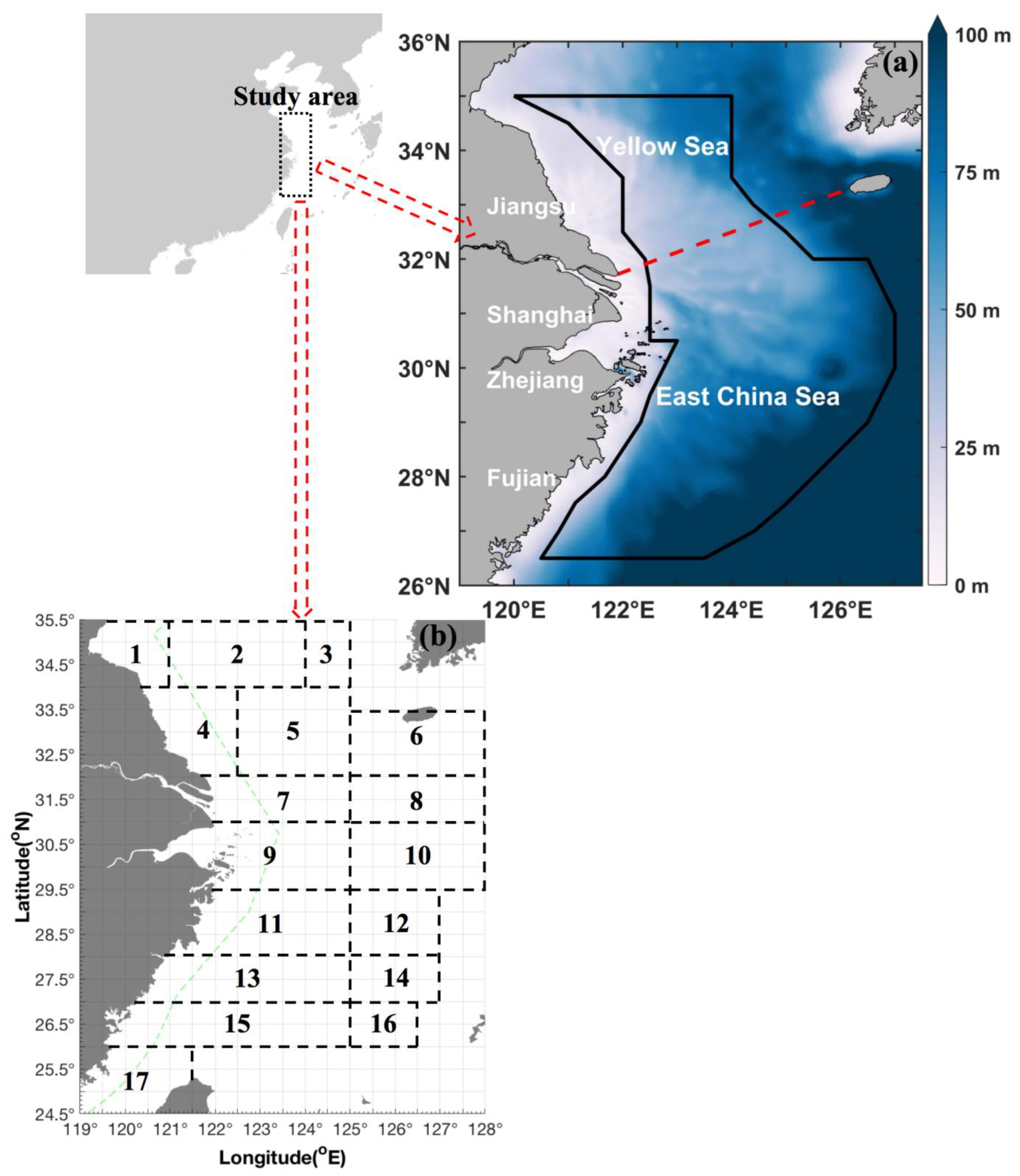
2.1. Sampling and Survey Procedures

Bottom-trawling surveys were conducted in the southern Yellow and East China Seas during 2018 and 2019. The surveys used a trawl net with a cod end mesh size of 20 mm that was towed by fisheries research vessels (Zhongkeyu 211 and 212) during the autumn (2–11 November 2018), winter (4–27 January 2019), spring (22 April–10 May 2019), and summer (13 August–27 September 2019). The study area covered 26.50°–35.00° N, 120.00°–127.00° E, and the sample trawls were conducted in a grid pattern with longitude and latitude spacings of 30 min × 30 min (Figure 1). The average trawl speed was 3 knots, and all tows were conducted for a duration of 1 h at each station. In total, 519 valid tows were included in this study (127 stations in autumn, 111 stations in winter, 141 stations in spring, and 140 stations in summer).
Environmental variables were measured at each station using a conductivity–temperature–depth profiler (SBE-19; SeaBird-Scientific, Bellevue, WA, USA). Sea surface temperature (SST), sea surface salinity (SSS), and sea surface dissolved oxygen (SSDO) were measured at 3 m below the surface, while sea bottom temperature (SBT), sea bottom salinity (SBS), and sea bottom dissolved oxygen (SBDO) were measured 2 m above the sea bottom at sea depths <50 m and at 2–4 m above the bottom at sea depths >50 m. Ottersen et al. (2010) [22] suggested that oceanographic parameters such as SST, SBT, SSS, and SBS are very important for ocean circulation patterns, vertical mixing, availability of nutrients, and subsequent marine ecosystem primary production, which appear to be the leading indicators and important drivers of marine fishery resource fluctuations.
The catches from each station were transported to the laboratory for analysis. The total number and weight of both species were counted and weighed to the nearest 0.10 g of wet weight; the catch density was calculated as the biomass density per unit of sampling time CPUEw (g·h−1) and density per unit of sampling time CPUEn (ind·h−1). The total values of CPUEw and CPUEn across the sampling sites are detailed in Table 1. The average individual weight (AIW) was defined as the CPUEw divided by the CPUEn at each station.

2.2. Ensemble Model, Selection of Environmental Variables, and Evaluations

The species distribution model is widely used as a tool for analyzing the spatio-temporal distribution patterns of marine living organisms, modelling with key steps including problem scoping, problem conceptualization, model formulation and evaluation, model application, and model perpetuation [23].
We used ten algorithms to predict the habitat distribution of both species based on the collected data: artificial neural network (ANN), classification tree analysis (CTA), flexible discriminant analysis (FDA), generalized additive model (GAM), generalized boosting model (GBM), generalized linear model (GLM), multiple adaptive regression splines (MARS), random forest (RF), surface range envelope (SRE), and extreme gradient boosting training (XGBOOST). These were combined into a species distribution model (SDM) to describe and forecast the relationship between the species and environmental variables. Araujo and New (2007) reported that combining these ten models into the SDM was more advantageous compared with single models, improving the robustness of the prediction and decreasing analysis bias, thereby yielding more confidence in the predictions [24]. We used the mean data of the surveyed four months to produce the annual model and used different seasonal data to produce the seasonal models. All the data used in the models were obtained from the surveys conducted as part of this study.
We used the ‘biomod2’ package in the ensemble SDM platform. To run the model, the data set was separated into categories of 0 (absence) and 1 (presence), and an 80%:20% split was then randomly applied for training and testing the data independently to construct the ten algorithms using the random cross-validation method [25]. The performance of each algorithm was assessed by the index of the area under the receiver operating characteristic curve (ROC) and the true skill statistic (TSS) [26]. Among these models, we selected those that performed best (a threshold value of the receiver operating characteristic curve (AUC) > 0.8) and combined them into an ensemble model using the weighted average method. The weighted average method is a method of weighting the mean of probabilities over the selected algorithms. Single algorithms are combined into an ensemble model based on the weighted average method. The single algorithm is weighted according to the obtained assessment scores.
Shared Socioeconomic Pathways (SSPs) are used to explore how societal choices will affect greenhouse gas emissions. SSPs include a world of sustainability-focused growth and equality (SSP1); a ‘middle of the road’ world where trends broadly follow their historical patterns (SSP2); a fragmented world of ‘resurgent nationalism’ (SSP3); a world of ever-increasing inequality (SSP4); and a world of rapid and unconstrained growth in economic output and energy use (SSP5) (details can be found at https://www.carbonbrief.org/explainer-how-shared-socioeconomic-pathways-explore-future-climate-change/ (accessed on 20 March 2025)).
Future climate data were obtained from CMIP6 (https://pcmdi.llnl.gov/CMIP6/ (accessed on 20 March 2025)), and predicted environmental data, such as SST, SBT, SSS, and SBS, were obtained from Bio-ORACLE (https://bio-oracle.org/index.php (accessed on 20 March 2025)). Four SSP scenarios (SSP1-2.6, SSP2-4.5, SSP3-7.0, and SSP5-8.5) for 2040–2050 (the 2050s) and 2090–2100 (the 2090s) were used in this study [27]. Bias corrections were performed for SST, SSS, SBT, and SBS, given that such correction of climate model raw data is essential to enhance the credibility of habitat distributions under future climate scenarios [28]. The delta method is a prevalent technique in fisheries habitat prediction that effectively mitigates such biases [29]. We used this approach to calculate climate differences between current and future data sets by applying corrections to the raw data. Specifically, the delta method leverages discrepancies between observed and simulated baseline conditions to adjust simulations for time (t) periods (here, 2040–2050 and 2090–2100) [30].
Bias correction for time t in geographical location x was conducted using Equation (1):
D s i m D M x , t = D e m p x , 0 + D s i m r a w x , t D s i m r a w x , 0 = D s i m r a w x , t + D e m p x , 0 D s i m r a w x , 0
where D e m p x , 0 D s i m r a w x , 0 represents the bias as the anomaly between observed and simulated environmental data at geographical location x and D s i m D M x , t denotes the bias-corrected temperature forecasts that were calculated by adding the bias to the simulated environmental data for time t in geographical location x.

3. Results and Discussion

3.1. Seasonal Variations in Environmental Variables of Both Species

Previous work recorded adult E. berryi occurring at a depth of up to 60 m on the Pacific side of mainland Japan [18]. In our study, E. berryi was found at a minimum and maximum measured depth of 55 m and 84 m, respectively, in summer and at minimum depth of 58 m and maximum depth of 107 m in autumn, indicating a potential seasonal expansion from shallower inshore to deeper offshore areas (Table 2). By contrast, E. morsei was found in shallower water areas in spring, expanding to the whole survey area during autumn and winter (Table 2).
The SBT ranges of E. berryi were similar between autumn and winter, with the highest values in autumn and winter being similar to the lowest value in summer. The SBT ranges of E. morsei were similar in spring, autumn, and winter, being highest from autumn to winter to spring. The SSS ranges of E. berryi and E. morsei were similar across the seasons. The SBS values for E. berryi were higher in summer compared with autumn and winter, a pattern also seen for E. morsei (Table 2). The SSDO and SBDO ranges were similar for each species in each of the seasons (Table 2).

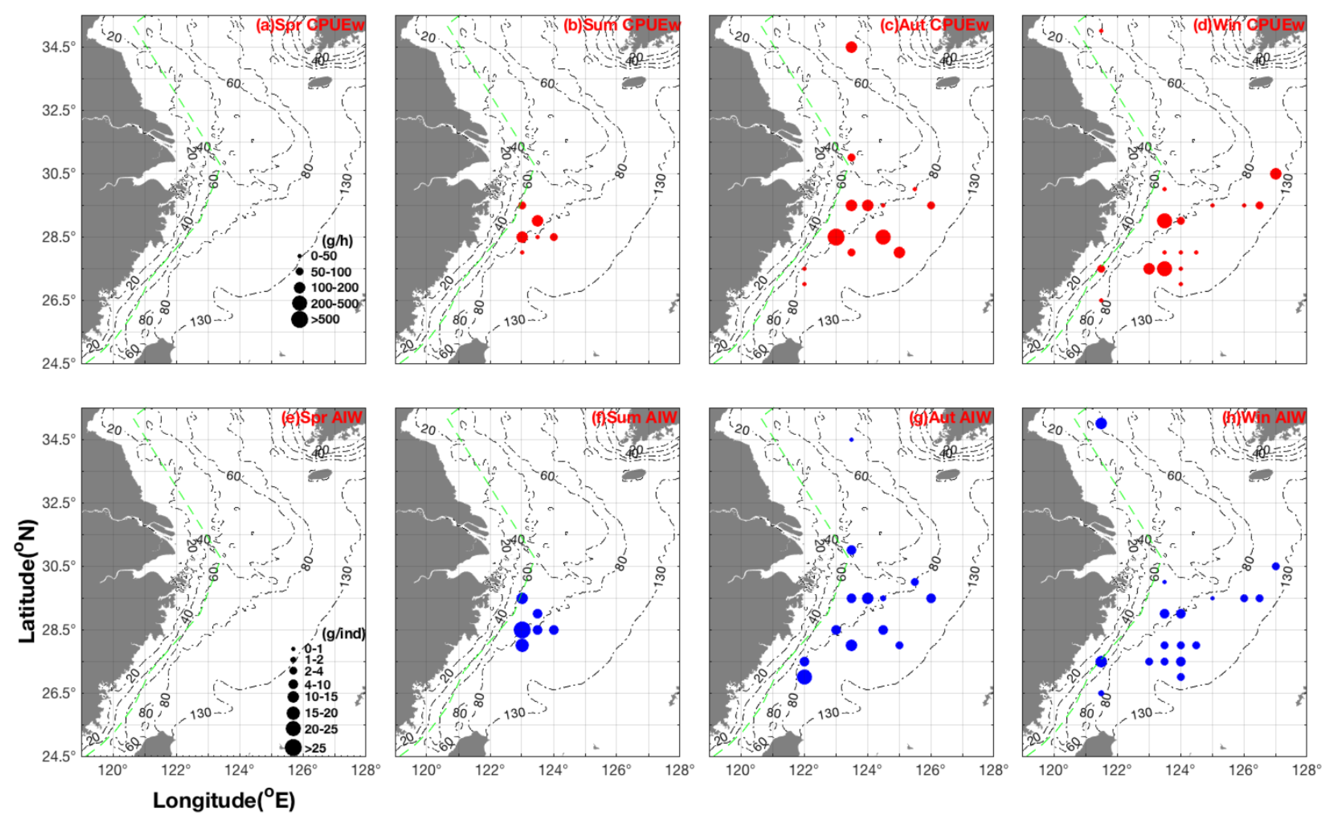
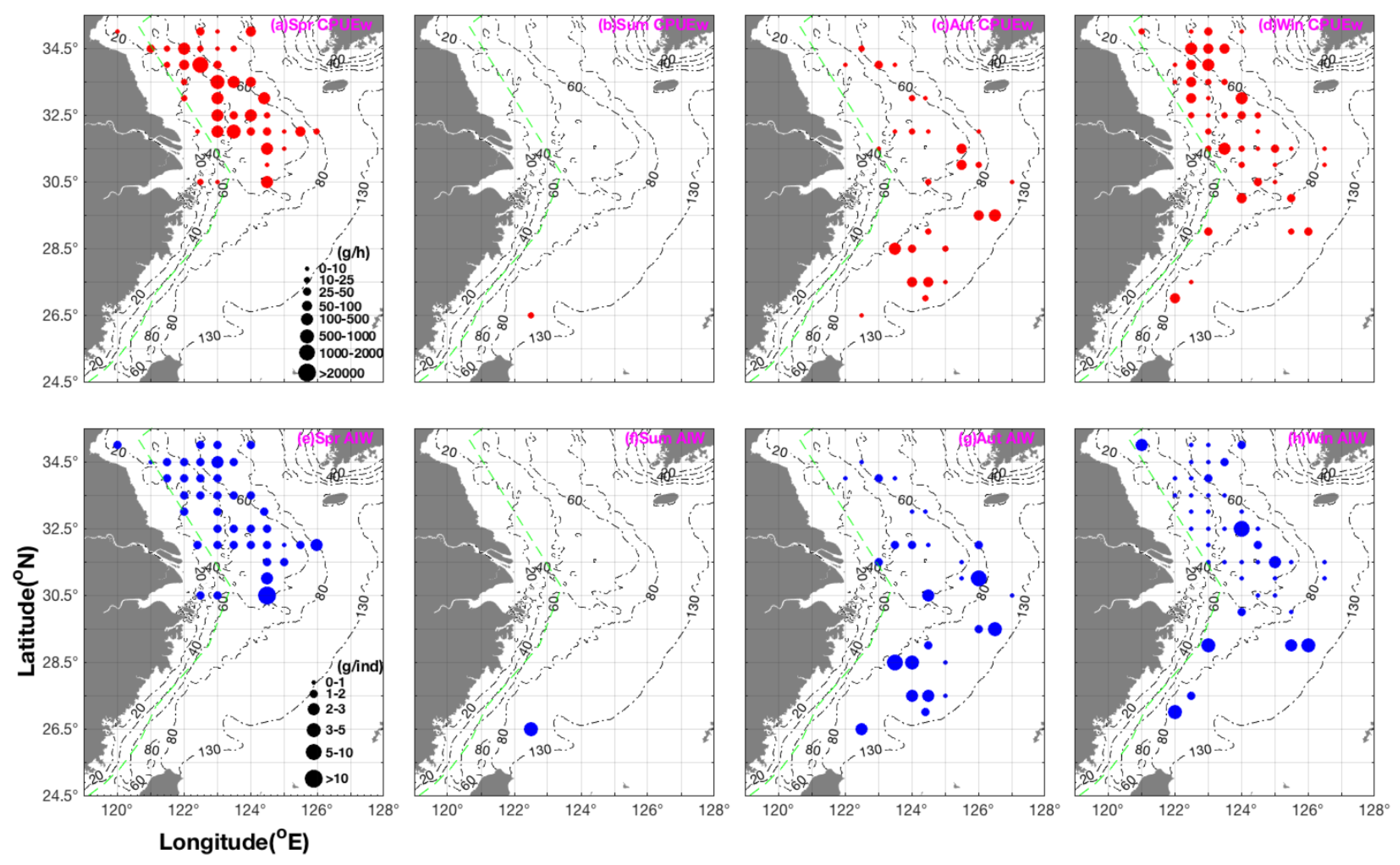
3.2. Seasonal Spatial Distribution Patterns and Characteristics of CPUEw and AIW

The highest biomass of E. berryi occurred in the Yushan fishing ground in summer, with a higher biomass in northern than in southern Yushan. During the summer, larger E. berryi also inhabited coastal water areas (Figure 2). In autumn, most E. berryi remained in the Yushan fishing ground, adopting a wide distribution from Haizhou Bay to Wentai fishing grounds; both E. berryi biomass and individual sizes increased from the southern Yellow Sea to the East China Sea, with the longitudinal mean CPUEw and AIW increasing in the order of 125°–126° E→124°–124.5° E→123.5° E→122°–123° E (Figure 2). During the winter, the highest E. berryi biomass occurred in the Wentai fishing ground, with a spatial distribution range that included fishing grounds from Haizhou Bay to Mindong; most E. berryi were found in a longitudinal range of 123°–123.5° E, with the mean AIW increasing in a longitudinal order of 125°–127° E→124°–124.5° E→123°–123.5° E→121.5° E (Figure 2). The E. berryi spawning season has been reported to occur from late April to July in Aichi, Japan [31], and from March to December in Taiwan [32], with Jolly et al. (2022) reporting that E. berryi adults were found from April to June in the southern and the Pacific Ocean side of mainland Japan [18]. In the current study, the highest CPUEw values occurred in the order of autumn > winter > summer, with mean AIW decreasing from summer to autumn to winter (Table 1).
E. morsei was mainly distributed in the southern Yellow and northern East China Seas in spring, with smaller and larger individual sizes occurring in inshore and offshore areas, respectively. The latitudinal mean CPUEw continuously increased in the order of 35° N→34.5° N→34° N→33.5° N, with the greatest biomass found at 122.5° E (Figure 3). In summer, this species was only recorded at one station (26.5° N 122.5° E). In autumn, smaller individuals were found in the latitudinal range of 34°–34.5° N, with smaller and larger individuals mainly found in northern and southern study areas, respectively; the greatest biomass occurred at 126°–127° E, with smaller individuals found at 125°–125.5° E (Figure 3). In winter, AIW ranged from 0.81 to 1.26 g ind−1 at 34.5° N and 1.2 to 4.844 g ind−1 at 27°–29° N, indicating a potential nursery function of these locations. The highest biomass occurred at 34° N and 122.5°–123.5° E (Figure 3). Our results indicated a relatively low biomass and numbers caught in autumn and winter, suggesting that E. morsei juveniles bury themselves under the substrate and, thus, avoid capture by trawl surveys. The order of the highest CPUEw values was spring > winter > autumn, whereas that for mean AIW was summer > spring + autumn > winter (Table 1).

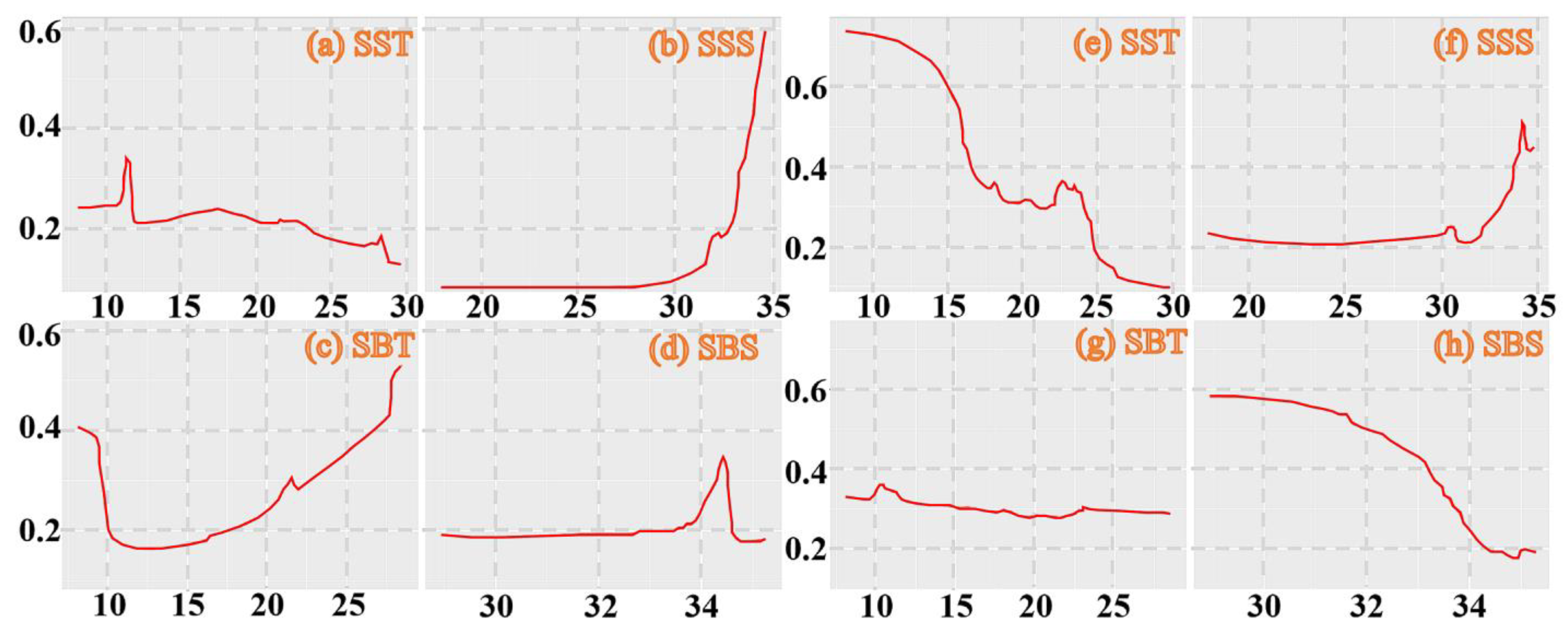
3.3. Model Evaluation and Suitable Habitat and Environmental Factors

The CTA, FDA, GAM, GBM, GLM, RF, XGBOOST, and ensemble models showed that variability in SSS was most important in determining the distribution of E. berryi, whereas the ANN algorithm suggested that variability in SBT was most important, and the MARS and SRE algorithms highlighted variability in SBS as being most important (Figure S1 in the Supplementary Material online). By contrast, all algorithms showed that variability in SST was the most important factor determining the distribution of E. morsei (Figure S1). Environmental factors, such as water temperature and other physico-chemical parameters, play a vital role in shaping species distribution and habitat suitability. Seasonal fluctuations in these parameters, as observed in previous studies (e.g., Naeem et al., 2011) [33], indicate that climate-induced changes could further impact habitat conditions for E. berryi and E. morsei. This highlights the need for continuous monitoring of environmental variables to better understand the ecological responses of these species under different climate scenarios. In terms of TSS and ROC, RF was the best model (Figures S2 and S3).
In terms of suitable habitat range, E. berryi expanded northward during autumn and winter compared with their location during the summer. By contrast, E. morsei was concentrated in the southern Yellow and northern East China Seas during the spring and winter compared with occurring throughout the study area during the summer and autumn (Figures S4–S6). The suitable habitat area for E. morsei extended to the south in winter to spring, becoming even more southerly during the summer and autumn (Figures S4–S6).
The suitable environmental variables predicted for the study year for E. berryi were as follows: 10–30 °C SST, >28 °C SBT, >33‰ SSS, and ~34.5‰ SBS, whereas, for E. morsei, these were 10–15 °C SST, >10–25 °C SBT, >34‰ SSS, and 29–32‰ SBS (Figure 4).
Choe (1966) [31] reported that the embryonic period of E. berryi was 20 days at 23.5–24.0 °C, with mature E. berryi observed spawning fertilized clutches repeatedly over a period of 100 days at 20 °C. In our study, E. berryi was most numerous in regions during the summer where the SBT was 25.29–28.02 °C and SBS was 33.43–34.04‰ compared with an SBT of 9.47 °C and SBS of 32.75‰ and SBT 20.99–21.69 °C and SBS of 34.07–34.50‰ during the autumn and an SBT of 17.13–20.36 °C and SBS of 34.23–34.46‰ during the winter (Figure 5a).
Watanabe (1997) [34] reported that the embryonic period of E. morsei was 32 days at 20 °C. In our study, E. morsei was most numerous in regions during the spring with an SBT of 12.59–12.83 °C and SBS of 32.95–32.91‰, during the summer in areas with a SBT of 19.54 °C and SBS of 34.43‰ compared with an SBT of 21.98–22.70 °C and SBS 33.80–33.60‰ in autumn and SBT of 10.51–13.49 °C and SBS 31.69–33.42‰ in winter (Figure 5b).

3.4. Habitat Predictions Under Different Climate Projections

Currently, the habitat area suitable for E. morsei is larger than that for E. berryi, with the latter mainly concentrated in the Mindong-Yushan fishing grounds. Under the SSP585-2050 scenario, the habitat area suitable for E. berryi would expand more northward. The habitat area suitable for E. morsei would retreat northward under the SSP370-2100 and SSP585-2100 scenarios (Table 3; Figures S7–S9).
Under the various climate scenarios, the area of habitat suitable for E. morsei would be smaller than that for E. berryi. Under SSP126-2050, SSP245-2050, and SSP585-2050, a reduction in area of <5% would occur for E. berryi, whereas a reduction of 5–10% would occur under scenarios SSP126-2100 and SSP370-2050, and a reduction of >10% would occur under scenarios SSP245-2100, SSP370-2100, and SSP585-2100 (Table 3).
By contrast, there would be more areas of suitable habitat for E. morsei than for E. berryi under scenarios SSP126-2050 and SSP245-2050 versus fewer areas of suitable habitat under scenarios SSP126-2100, SSP245-2100, SSP370-2050, SSP370-2100, SSP585-2050, and SSP585-2100. Increases in suitable habitat of <5% for E. morsei would occur under scenarios SSP126-2100, SSP245-2100, SSP370-2050, SSP370-2100, SSP585-2050, and SSP585-2100, whereas increases >5% would occur under SSP126-2050 and SSP245-2050. Increases in suitable habitat of <10% for E. berryi would occur under SSP126-2050, SSP126-2100, SSP245-2050, SSP370-2050, and SSP585-2050, whereas increases >10% would occur under SSP245-2100, SSP370-2100, and SSP585-2100 (Table 3).
In terms of total changes in area, increases in area of <10% for E. berryi would occur under SSP126-2050, SSP245-2050, and SSP585-2050, whereas reduced area percentages of <10% would occur under SSP126-2100, SSP245-2100, SSP370-2050, SSP370-2100, and SSP585-2100, with the percentage of reduced area being greatest under SSP585-2100. E. morsei would experience greater reductions in the amount of suitable habitat under all scenarios (>90% under SSP245-2100 and SSP585-2100; 50–90% under SSP245-2050, SSP370-2050, SSP370-2100, and SSP585-2100; and <50% under SSP126-2050 and SSP126-2100; Table 3).
In the East China Sea region, the distribution of Sepia esculenta was found to be more northerly than previously reported [35]. By the 2050s, the joint distribution areas of Loliolus beka and Loliolus uyii were predicted to expand to the central East China Sea and the southern Yellow Sea [36]. The habitat range of Sepiella maindroni will greatly decrease under the case of SSP585 [37]. The core habitat of AmphiOctopus ovulum is expected to expand to the northeast and southwest independently [38]. The annual mean habitat area of AmphiOctopus fangsiao will shrink significantly [39]. The habitat area range of Abralia multihamata will move poleward from spring to winter [40].
Both species are small in size and currently not commercially exploited. However, their small size would be economically advantageous because culture conditions would be required on a smaller scale with lower costs and fewer facility requirements compared with those used for pelagic and large-sized species. E. berryi and E. morsei are also suitable model species for reproductive studies because of their short lifespan (5–8 months). In addition, they are more easily maintained in laboratory conditions compared with other larger species. This study has some limitations. Specifically, the methods used in this study have potential risk of overfitting in predicting future distributions of the species under different climate scenarios [41]. This might cause bias about the spatial-temporal distribution patterns of both species owing to variability in trawling efficiency and others. Future work should focus on continuous population monitoring for both species, especially whether the population size of E. berryi alters compared with that of E. morsei in response to climate change, which can cause species succession and transformation of ecosystem functions in this study area.

4. Conclusions

There are several conclusions reached by our study. During the summer, larger E. berryi were found in shallower water areas, which then migrated northward during the autumn and winter. In autumn, there was a larger biomass of E. berryi, with increased numbers of larger individuals, in the southern Yellow Sea compared with East China Sea, concentrated in inshore areas to overwinter. During spring, E. morsei were concentrated for breeding in a small area, with an SBT of 12.59–12.83 °C and SBS of 32.95–32.91‰. During the autumn and winter, this species migrated southward from the southern Yellow and northern East China Seas. It might be that the fishing grounds of Haizhou Bay and Wentai-Yushan are nursery grounds for this species, whereas offshore areas provide overwintering grounds. SSS appeared to be the most important determinant of suitable habitat for E. berryi, whereas this was SST for E. morsei. In this study, we used ensemble models produced by very often used algorithms to identify the seasonal spatial distribution patterns across the seasons and distribution range variations in both species under different climate scenarios. In the future, we will discuss the relationship between single algorithms and an ensemble model in the case of the available verified survey data. The biological ecological information of both species obtained in this study can offer insights into how small-size squids are varying corresponding to climate changes and, thus, offer key insights to fishery managers about ecosystem-based management incorporating into climate changes. Finally, we appeal that ocean governance should consider climate change and forecasting to drive transformative, sustainable, and inclusive ocean care.

Supplementary Materials

The following supporting information can be downloaded at: https://www.mdpi.com/article/10.3390/biology14040327/s1, Figure S1. Box plot of variable important against environmental variables including sea bottom salinity (SBS), sea bottom temperature (SBT), sea surface salinity (SSS), and sea surface temperature (SST), of Euprymna berryi (right panels: a–k) and Euprymna morsei (left panels: l–v), produced by the algorithms of (a,l) artificial neural network (ANN), (b,m) classification tree analysis (CTA), (c,n) flexible discriminant analysis (FDA), (d,o) generalized additive model (GAM), (e,p) generalized boosting model (GBM), (f,q) generalized linear model (GLM), (g,r) multiple adaptive regression splines (MARS), (h,s) random forest (RF), (i,t) surface range envelope (SRE), (j,u) extreme gradient boosting training (XGBOOST), and (k,v) ensemble model. Figure S2. Calibration percentage (%) of TSS and ROC for the species Euprymna berryi (upper panels) and Euprymna morsei (bottom panels) in different algorithms of artificial neural network (ANN), classification tree analysis (CTA), flexible discriminant analysis (FDA), generalized additive model (GAM), generalized boosting model (GBM), generalized linear model (GLM), multiple adaptive regression splines (MARS), random forest (RF), surface range envelope (SRE), and extreme gradient boosting training (XGBOOST). Figure S3. The ratio values of TSS against ROC for the species Euprymna berryi (left panel) and Euprymna morsei (right panel) with x-direction and y-direction error bars produced by different methods, including artificial neural network (ANN), classification tree analysis (CTA), flexible discriminant analysis (FDA), generalized additive model (GAM), generalized boosting model (GBM), generalized linear model (GLM), multiple adaptive regression splines (MARS), random forest (RF), surface range envelope (SRE), and extreme gradient boosting training (XGBOOST), displayed by the colors of black, blue, green, cyan, red, pink, dark yellow, dark blue, purple, and red–brown. Figure S4. Seasonal spatial distribution patterns of Euprymna berryi (upper panels: a–d) and Euprymna morsei (bottom panels: e–h) in spring to winter in the study area predicted with the ensemble model consisting of the algorithms of artificial neural network (ANN), classification tree analysis (CTA), flexible discriminant analysis (FDA), generalized additive model (GAM), generalized boosting model (GBM), generalized linear model (GLM), multiple adaptive regression splines (MARS), random forest (RF), surface range envelope (SRE), and extreme gradient boosting training (XGBOOST). The color of blue to green indicates the range from low to high suitability independently. Figure S5. The predicted habitat suitability for Euprymna berryi in different seasons (spring, summer, autumn, winter). The red and blue area indicates the suitability index of 0.7–1 and 0–0.7 independently. Figure S6. The predicted habitat suitability for Euprymna morsei in different seasons (spring, summer, autumn, winter). The red and blue area indicates the suitability index of 0.7–1 and 0–0.7 independently. Figure S7. Predicted spatial habitat distribution patterns of Euprymna berryi (a–i) and Euprymna morsei (j–r) in the cases of annual mean habitat, SSP1-2.6 in 2050, SSP1-2.6 in 2100, SSP2-4.5 in 2050, SSP2-4.5 in 2100, SSP3-7.0 in 2050, SSP3-7.0 in 2100, SSP5-8.5 in 2050, and SSP5-8.5 in 2100. The bar colored in blue to green indicates the range from low to high suitability. Figure S8. The predicted habitat suitability for Euprymna berryi in different climate scenarios: (a) current; (b) SSP1-2.6 in 2050; (c) SSP1-2.6 in 2100; (d) SSP2-4.5 in 2050; (e) SSP2-4.5 in 2100; (f) SSP3-7.0 in 2050; (g) SSP3-7.0 in 2100; (h) SSP5-8.5 in 2050; and (i) SSP5-8.5 in 2100. The red and blue area indicates the suitability index of 0.7–1 and 0–0.7 independently. Figure S9. The predicted habitat suitability for Euprymna morsei in different climate scenarios: (a) current; (b) SSP1-2.6 in 2050; (c) SSP1-2.6 in 2100; (d) SSP2-4.5 in 2050; (e) SSP2-4.5 in 2100; (f) SSP3-7.0 in 2050; (g) SSP3-7.0 in 2100; (h) SSP5-8.5 in 2050; and (i) SSP5-8.5 in 2100. The red and blue area indicates the suitability index of 0.7–1 and 0–0.7 independently.

Author Contributions

M.X. and L.Y. contributed to the development, planning, and data collection; X.S. and Y.L. contributed to the data interpretation. All authors contributed to the writing of the manuscript. All authors have read and agreed to the published version of the manuscript.

Funding

This research was supported by the National Key R&D Program of China (Grant/Award Numbers: 2024YFD2400404).

Institutional Review Board Statement

Ethical review and approval were waived for this study due to the lack of involvement with an endangered species.

Informed Consent Statement

Not applicable.

Data Availability Statement

The data sets used and/or analyzed during the current study are available from the corresponding author on reasonable request.

Acknowledgments

The authors wish to thank the crews of the fishing boats for their help with field sampling; members of the Key Laboratory of East China Sea and the Oceanic Fishery Resources Exploitation, Ministry of Agriculture and Rural Affairs; and Wenquan Sheng for constructive discussions and encouragement.

Conflicts of Interest

The authors declare no conflicts of interest.

References

  1. Yang, Y.; Gao, W.; Han, Y.; Zhou, T. Predicting the Impact of Climate Change on the Distribution of North China Leopards (Panthera pardus japonensis) in Gansu Province Using MaxEnt Modeling. Biology 2025, 14, 126. [Google Scholar] [CrossRef] [PubMed]
  2. Thomas, C.D.; Cameron, A.; Green, R.E.; Bakkenes, M.; Beaumont, L.J.; Collingham, Y.C.; Erasmus, B.F.N.; De Siqueira, M.F.; Grainger, A.; Hannah, L.; et al. Extinction risk from climate change. Nature 2004, 427, 145–148. [Google Scholar] [PubMed]
  3. Brown, J.H.; Gillooly, J.F.; Allen, A.P.; Savage, V.M.; West, G.B. Toward a metabolic theory of ecology. Ecology 2004, 85, 1771–1789. [Google Scholar]
  4. Chen, I.C.; Hill, J.K.; Ohlemuller, R.; Roy, D.B.; Tomas, C.D. Rapid range shifts of species associated with high levels of climate warming. Science 2011, 333, 1024–1026. [Google Scholar]
  5. Berg, M.P.; Kiers, E.T.; Driessen, G.; Van Der HeijdenJ, M.; Kooi, B.W.; Kuenen, F.; Liefting, M.; Verhoef, H.A.; Ellers, J. Adapt or disperse: Understanding species persistence in a changing world. Glob. Change Biol. 2010, 16, 587–598. [Google Scholar]
  6. Xue, K.M.; Yuan, M.J.; Shi, Z.; Qin, Y.; Deng, Y.E.; Cheng, L.; Wu, L.; He, Z.; Van Nostrand, J.D.; Bracho, R.; et al. Tundra soil carbon is vulnerable to rapid microbial decomposition under climate warming. Nat. Clim. Change 2016, 6, 595–600. [Google Scholar]
  7. Cardinale, B.J.; Duffy, J.E.; Gonzalez, A.; Hooper, D.U.; Perrings, C.; Venail, P.; Narwani, A.; Mace, G.M.; Tilman, D.; Wardle, D.A.; et al. Biodiversity loss and its impact on humanity. Nature 2012, 486, 59–67. [Google Scholar]
  8. Miller, T.E.; Gornish, E.S.; Buckley, H.L. Climate and coastal dune vegetation: Disturbance, recovery, and succession. Plant Ecol. 2010, 206, 97–104. [Google Scholar]
  9. Guo, X.; Feng, J.; Shi, Z.; Zhou, X.; Yuan, M.; Tao, X.; Hale, L.; Yuan, T.; Wang, J.; Qin, Y.; et al. Climate warming leads to divergent succession of grassland microbial communities. Nat. Clim. Change 2018, 8, 813–818. [Google Scholar]
  10. Wang, X.; Qiu, Y.; Du, F.; Liu, W.; Sun, D.; Chen, X.; Yuan, W.; Chen, Y. Roles of fishing and climate change in long-term fish species succession and population dynamics in the outer Beibu Gulf, South China Sea. Acta Oceanol. Sinica 2019, 38, 1–8. [Google Scholar]
  11. Ma, S.; Liu, Y.; Li, J.; Fu, C.; Ye, Z.; Sun, P.; Yu, H.; Cheng, J.; Tian, Y. Climate-induced long-term variations in ecosystem structure and atmosphere-ocean-ecosystem processes in the Yellow Sea and East China Sea. Prog. Oceanogr. 2019, 175, 183–197. [Google Scholar]
  12. Cai, R.; Tan, H.; Qi, Q. Impacts of and adaptation to inter-decadal marine climate change in coastal China seas. Int. J. Climatol. 2016, 36, 3770–3780. [Google Scholar]
  13. Pisano, A.; Marullo, S.; Artale, V.; Falcini, F.; Yang, C.; Leonelli, F.E.; Santoleri, R.; Buongiorno Nardelli, B. New Evidence of Mediterranean Climate Change and Variability from Sea Surface Temperature Observations. Remote Sens. 2020, 12, 132. [Google Scholar] [CrossRef]
  14. Darmaraki, S.; Denaxa, D.; Theodorou, I.; Livanou, E.; Rigatou, D.; Raitsos, E.D.; Stavrakidis-Zachou, O.; Dimarchopoulou, D.; Bonino, G.; McAdam, R.; et al. Marine Heatwaves in the Mediterranean Sea: A Literature Review. Mediterr. Mar. Sci. 2024, 25, 586–620. [Google Scholar]
  15. Reid, A.; Jereb, P. Family Sepiolidae. In Cephalopods of the World; FAO: Rome, Italy, 2005; Available online: http://www.fao.org/3/ac479e/ac479e00.htm (accessed on 8 February 2025).
  16. McFall-Ngai, M.; Montgomery, M.K. The anatomy and morphology of the adult bacterial light organ of Euprymna scolopes Berry (Cephalopoda: Sepiolidae). Biol. Bull. 1990, 179, 332–339. [Google Scholar] [PubMed]
  17. Nabhitabhata, J.; Nishiguchi, M.K. Euprymna hyllebergi and Euprymna tasmanica. In Cephalopod Culture; Springer: Dordrecht, The Netherlands, 2014; pp. 253–269. [Google Scholar]
  18. Jolly, J.; Hasegawa, Y.; Sugimoto, C.; Zhang, L.; Kawaura, R.; Sanchez, G.; Gavriouchkina, D.; Marlétaz, F.; Rokhsar, D. Lifecycle, culture, and maintenance of the emerging cephalopod models Euprymna berryi and Euprymna morsei. Front. Mar. Sci. 2022, 9, 1039775. [Google Scholar]
  19. Sundaram, S.; Sreeram, M.P. First record of sepiolid squid, Euprymna berryi Sasaki, 1929 from the west coast of India. J. Mar. Biol. Assoc. India 2008, 50, 221–223. [Google Scholar]
  20. Singley, C. Euprymna scolopes. In Cephalopod Life Cycles; Academic Press: London, UK, 1983; Volume 1, pp. 69–74. [Google Scholar]
  21. Norman, M.D. Cephalopods, A World Guide; ConchBooks: Hackenheim, Germany, 2000; pp. 1–320. [Google Scholar]
  22. Ottersen, G.; Kim, S.; Huse, G.; Polovina, J.J.; Stenseth, N.C. Major pathways by which climate may force marine fish populations. J. Mar. Syst. 2010, 79, 343–360. [Google Scholar]
  23. Jakeman, A.J.; Elsawah, S.; Wang, H.H.; Hamilton, S.H.; Melsen, L.; Grimm, V. Towards normalizing good practice across the whole modeling cycle: Its instrumentation and future research topics. Socio-Environ. Syst. Model. 2024, 6, 18755. [Google Scholar]
  24. Araujo, M.; New, M. Ensemble forecasting of species distributions. Trends. Ecol. Evol. 2007, 22, 42–47. [Google Scholar] [PubMed]
  25. Liu, S.; Liu, Y.; Alabia, I.D.; Tian, Y.; Ye, Z.; Yu, H.; Li, J.; Cheng, J. Impact of Climate Change on Wintering Ground of Japanese Anchovy (Engraulis japonicus) Using Marine Geospatial Statistics. Front. Mar. Sci. 2020, 7, 604. [Google Scholar]
  26. Liu, S.; Liu, Y.; Teschke, K.; Hindell, M.A.; Downey, R.; Woods, B.; Kang, B.; Ma, S.; Zhang, C.; Li, J.; et al. Incorporating mesopelagic fish into the evaluation of conservation areas for marine living resources under climate change scenarios. Mar. Life Sci. Technol. 2024, 6, 68–83. [Google Scholar]
  27. Liu, S.; Tian, Y.; Liu, Y.; Alabia, I.D.; Cheng, J.; Ito, S. Development of a prey-predator species distribution model for a large piscivorous fish: A case study for Japanese Spanish mackerel Scomberomorus niphonius and Japanese anchovy Engraulis japonicus. Deep Sea Res. Part II 2023, 207, 105227. [Google Scholar]
  28. Liu, S.; Liu, Y.; Xing, Q.; Li, Y.; Tian, H.; Luo, Y.; Ito, S.; Tian, Y. Climate change drives fish communities: Changing multiple facets of fish biodiversity in the Northwest Pacific Ocean. Sci. Total Environ. 2024, 955, 176854. [Google Scholar]
  29. Silva, C.; Yáñez, E.; Barbieri, M.A.; Bernal, C.; Aranis, A. Forecasts of swordfish (Xiphias gladius) and common sardine (Strangomera bentincki) off Chile under the A2 IPCC climate change scenario. Prog. Oceanogr. 2015, 134, 343–355. [Google Scholar]
  30. Cheung, W.W.L.; Brodeur, R.D.; Okey, T.A.; Pauly, D. Projecting future changes in distributions of pelagic fish species of Northeast Pacific shelf seas. Prog. Oceanogr. 2015, 130, 19–31. [Google Scholar]
  31. Choe, S. On the eggs, rearing, habits of the fry, and growth of some Cephalopoda. Bull. Mar. Sci. 1966, 16, 330–348. [Google Scholar]
  32. Huang, C.P. Species Diversity of the Genus Euprymna Steenstrup, 1887 in Taiwan and Reproductive Cycle of Euprymna berryi Sasaki, 1929. Master’s Thesis, National Chung Hsing University, Taiwan, China, 2006. [Google Scholar]
  33. Naeem, M.; Salam, A.; Ashraf, M.; Imran, M.; Ahmed, M.; Khan, M.J.; Ayaz, M.M.; Ali, M.; Qayyum, M.; Ishtiaq, A. Studies on seasonal variations of physic-chemical parameters of fish farm at Govt. nursery unit, Muzaffargarh, Punjab, Pakistan. Proc. World Acad. Sci. Technol. 2011, 5, 60. [Google Scholar]
  34. Watanabe, K. Comparative Developmental Biology of the Embryonic and Early Life Stages of Decapod Cephalopods. Ph.D. Thesis, Tokyo University of Fisheries, Tokyo, Japan, 1997. (In Japanese). [Google Scholar]
  35. Xu, M.; Yang, L.; Liu, Z.; Zhang, Y.; Zhang, H. Seasonal and spatial distribution characteristics of Sepia esculenta in the East China Sea Region: Transfer of the central distribution from 29° N to 28° N. Animals 2024, 14, 1412. [Google Scholar] [CrossRef]
  36. Xu, M.; Feng, W.J.; Liu, Z.; Li, Z.G.; Song, X.J.; Zhang, H.; Zhang, C.L.; Yang, L.L. Seasonal-spatial distribution variations and predictions of Loliolus beka and Loliolus uyii in the East China Sea region: Implications from climate change scenarios. Animals 2024, 14, 2070. [Google Scholar] [CrossRef] [PubMed]
  37. Xu, M.; Liu, S.; Zhang, H.; Li, Z.; Song, X.; Yang, L.; Tang, B. Seasonal analysis of spatial distribution patterns and characteristics of Sepiella maindroni and Sepia kobiensis in the East China Sea Region. Animals 2024, 14, 2716. [Google Scholar] [CrossRef]
  38. Yang, L.; Xu, M.; Cui, Y.; Liu, S. Seasonal spatial distribution patterns of AmphiOctopus ovulum in the East China Sea: Current status future projections under various climate change scenarios. Front. Mar. Sci. 2025. accepted. [Google Scholar]
  39. Yang, L.L.; Xu, M.; Liu, Z.L.; Zhang, Y.; Cui, Y.; Li, S.F. Seasonal and spatial distribution of AmphiOctopus fangsiao and Octopus variabilis in the southern Yellow and East China Seas: Fisheries management implications based on climate scenario predictions. Reg. Stud. Mar. Sci. 2025, 83, 104072. [Google Scholar] [CrossRef]
  40. Xu, M.; Liu, S.; Yang, C.; Yang, L. Seasonal spatial distribution patterns of Abralia multihamata in the East China Sea Region: Predictions under various climate scenarios. Animals 2025, 15, 903. [Google Scholar] [CrossRef]
  41. Torrejón-Magallanes, J.; Ángeles-González, L.E.; Csirke, J.; Bouchon, M.; Morales-Bojórquez, E.; Arreguín-Sánchez, F. Modeling the Pacific chub mackerel (Scomber japonicus) ecological niche and future scenarios in the northern Peruvian Current System. Prog. Oceanogr. 2021, 197, 102672. [Google Scholar] [CrossRef]
Figure 1. Survey map information. (a) Map of the study area in the East China Sea region (26.50° N–35.00° N 120.00° E–127.00° E), denoted by a dark-blue solid line. The area includes the southern Yellow and East China Seas adjacent to the coastlines of Fujian, Zhejiang, Shanghai, and Jiangsu. The color bar denotes the depth range (0 m–100 m). The red-dashed line indicates the boundary between the Yellow Sea and East China Sea. (b) Fishing grounds: (1) Haizhou Bay, (2) Lianqingshi, (3) Liandong, (4) Lvsi, (5) Dasha, (6) Shawai, (7) Yangtze River mouth, (8) Jiangwai, (9) Zhoushan, (10) Zhouwai, (11) Yushan, (12) Yuwai, (13) Wentai, (14) Wenwai, (15) Mindong, (16) Minwai, and (17) Minzhong.
Biology 14 00327 g001
Figure 2. Seasonal distribution patterns of CPUEw (red; grouped into 0–50, 50–100, 100–200, 200–500, and >500 g h−1) and AIW (blue; grouped into 0–1, 1–2, 2–4, 4–10, 10–15, 15–20, 20–25, and >25 g ind−1) for Euprymna berryi. Abbreviations: AIW, average individual weight; CPUEw, catch per unit effort by weight.
Biology 14 00327 g002
Figure 3. Seasonal distribution patterns of CPUEw (red; grouped into 0–10, 10–25, 25–50, 50–100, 100–500, 500–1000, 1000–2000, and >20,000 g h−1) and AIW (blue; grouped into 0–1, 1–2, 2–3, 3–5, 5–10, and >10 g ind−1) for Euprymna morsei. Abbreviations: AIW, average individual weight; CPUEw, catch per unit effort by weight.
Biology 14 00327 g003
Figure 4. Responses of Euprymna berryi (ad) and Euprymna morsei (eh) to the environmental variables SST (10–30 °C), SSS (10–25 °C), SBT (20–35‰), and SBS (30–34‰). Abbreviations: SST, sea surface temperature; SBT, sea bottom temperature; SSS, sea surface salinity; SBS, sea bottom salinity.
Biology 14 00327 g004
Figure 5. Relationship between SBS (‰) and SBT (°C) for CPUEn sizes of Euprymna berryi (a) classified by group (0–20, 20–50, 50–100, 100–200, and 200–300 ind/h) and Euprymna morsei (b) classified by group (0–20, 20–50, 50–100, 100–200, 200–1000, and 1000–2000 ind/h). The data for spring, summer, autumn, and winter are denoted by blue, cyan, green, and brown–red solid circles, respectively. Abbreviations: CPUEn, catch per unit effort by number; SBS, sea bottom salinity; SBT, sea bottom temperature.
Biology 14 00327 g005
Table 1. Seasonal total biomass density (CPUEw) and density (CPUEn) of Euprymna berryi and Euprymna morsei in the study area.
SeasonEuprymna berryiEuprymna morsei
CPUEw (g·h−1)CPUEn (ind·h−1)CPUEw (g·h−1)CPUEn (ind·h−1)
Spring--8555.885243
Summer483.124811.13
Autumn3328.73636986.4662
Winter1612.864311664.71732
Table 2. Seasonal variation in environmental factors, biological indicators, and suitable habitat distribution range for Euprymna berryi and Euprymna morsei in the study area from autumn 2018 to summer 2019 a.
FactorEuprymna berryiEuprymna morsei
SummerAutumnWinterSpringSummerAutumnWinter
Depth (m)55–8458–10738–12613–8210416–11216–114
SST (°C)26.39–28.5618.92–23.6611.51–20.4212.85–17.3526.1118–24.568.21–20.52
SBT (°C)20.78–28.029.47–21.6911.52–20.369.64–17.9919.549.92–23.158.17–18.73
SSS (‰)31.92–34.0231.7–34.2332.06–34.5230.21–33.4934.0730.49–34.2931.5–34.51
SBS (‰)33.43–34.3432.75–34.5532.04–34.6130.55–33.9934.4331.37–35.0731.67–34.66
SSDO (mg/L)5.22–6.44/7.35–87.93–8.636.06/7.33–9.08
SBDO (mg/L)4.25–6.62/7.36–7.977.71–9.235.3/7.58–9.06
Mean CPUEw at collection stations (g/h)80.52256.0694.87213.911.136.5338.71
CPUEw range (g/h)25.2–154.961.35–2181.63.2–494.61.34–3203.211.12.4–178.820.5–297.6
Mean CPUEn at collection stations (ind/h)848.9225.35131.08324.5240.28
CPUEn range (ind/h)3–211–2881–1611–182431–1241–272
Mean AIW (g/ind)12.777.334.351.73.71.741.33
AIW range (g/ind)6.3–26.330.75–20.90.8–130.71–11.293.70.53–5.560.16–8.47
Suitable habitat range26.55°–29.35° N, 121.55°–126.95° E26.55°–32.65° N, 121.55°–126.95° E26.55°–32.25° N, 120.05°–126.95° E28.45°–34.95° N, 120.05°–126.45° E26.55°–34.95° N, 120.05°–125.65° E26.55°–34.95° N, 120.05°–126.95° E29.65°–34.95° N, 120.05°–126.25° E
a Abbreviations: SST, sea surface temperature; SBT, sea bottom temperature; SSS, sea surface salinity; SBS, sea bottom salinity; SSDO, sea surface dissolved oxygen; SBDO, sea bottom dissolved oxygen; CPUEw, catch per unit effort by weight; CPUEn, catch per unit effort by number; AIW, average individual weight.
Table 3. Percentages of habitat loss, gain, and overall habitat (gain minus loss) and most suitable habitat range for Euprymna berryi and Euprymna morsei under different climate scenarios.
Climate ScenarioLossGainTotalSuitable Habitat Range
CurrentE. berryi///26.55° N–29.35° N, 121.45° E–126.95° E
E. morsei///26.55° N–34.95° N, 120.05° E–126.95° E
SSP126-2050E. berryi−0.681%5.917%5.236%26.55° N–29.55° N, 121.55° E–126.95° E
E. morsei−61.571%18.09%−43.481%26.55° N–34.95° N, 120.05° E–126.95° E
SSP126-2100E. berryi−9.751%7.649%−2.102%26.55° N–29.35° N, 121.55° E–126.95° E
E. morsei−51.547%4.734%−46.813%26.55° N–34.95° N, 120.05° E–126.95° E
SSP245-2050E. berryi−0.584%4.885%4.301%26.55° N–29.55° N, 121.45° E–126.95° E
E. morsei−61.412%11.267%−50.145%26.55° N–34.95° N, 120.05° E–126.95° E
SSP245-2100E. berryi−19.015%10.568%−8.447%26.55° N–29.35° N, 121.55° E–126.95° E
E. morsei−91.775%0.344%−91.431%27.05° N–34.95° N, 120.05° E–126.25° E
SSP370-2050E. berryi−5.605%3.503%−2.102%26.55° N–29.45° N, 121.45° E–126.95° E
E. morsei−56.043%0.45%−55.594%26.55° N–34.95° N, 120.05° E–126.95° E
SSP370-2100E. berryi−24.912%18.276%−6.637%26.55° N–29.35° N, 121.55° E–126.95° E
E. morsei−70.114%0%−70.114%29.55° N–34.95° N, 120.05° E–126.25° E
SSP585-2050E. berryi−1.012%4.301%3.289%26.55° N–30.15° N, 121.55° E–126.95° E
E. morsei−68.659%3.227%−65.432%26.55° N–34.95° N, 120.05° E–126.95° E
SSP585-2100E. berryi−35.5%18.606%−16.894%26.55° N–29.45° N, 121.75° E–126.95° E
E. morsei−90.743%0%−90.743%29.65° N–34.95° N, 120.05° E–126.25° E
Disclaimer/Publisher’s Note: The statements, opinions and data contained in all publications are solely those of the individual author(s) and contributor(s) and not of MDPI and/or the editor(s). MDPI and/or the editor(s) disclaim responsibility for any injury to people or property resulting from any ideas, methods, instructions or products referred to in the content.

