Isotopic Niche Analysis of Long-Finned Pilot Whales (Globicephala melas edwardii) in Aotearoa New Zealand Waters

Simple Summary

Isotopic niche analyses can elucidate a species’ foraging ecology. Using isotopic values of δ¹³C, δ¹⁵N and δ³⁴S, the isotopic niche of long-finned pilot whales (Globicephala melas edwardii) in Aotearoa New Zealand was investigated for animals that stranded in six different events across two locations between 2009 and 2017. Generalised additive models revealed that stranding event was a stronger predictor for δ¹³C and δ¹⁵N values than body length, sex, or reproductive status, indicating that spatiotemporal differences explained isotopic variation of G. m. edwardii in New Zealand waters better than ontogenetic factors.

Abstract

The quantification of a species’ trophic niche is important to understand the species ecology and its interactions with the ecosystem it resides in. Despite the high frequency of long-finned pilot whale (Globicephala melas edwardii) strandings on the Aotearoa New Zealand coast, their trophic niche remains poorly understood. To assess the isotopic niche of G. m. edwardii within New Zealand, ontogenetic (sex, total body length, age, maturity status, reproductive group) and spatiotemporal (stranding location, stranding event, and stranding year) variation were investigated. Stable isotopes of carbon (δ¹³C) and nitrogen (δ¹⁵N) were examined from skin samples of 125 G. m. edwardii (67 females and 58 males) collected at mass-stranding events at Onetahua Farewell Spit in 2009 (n = 20), 2011 (n = 20), 2014 (n = 27) and 2017 (n = 20) and at Rakiura Stewart Island in 2010 (n = 19) and 2011 (n = 19). Variations in δ³⁴S values were examined for a subset of 36 individuals. General additive models revealed that stranding event was the strongest predictor for δ¹³C and δ¹⁵N values, whilst sex was the strongest predictor of δ³⁴S isotopic values. Although similar within years, δ¹³C values were lower in 2014 and 2017 compared to all other years. Furthermore, δ¹⁵N values were higher within Farewell Spit 2017 compared to any other stranding event. This suggests that the individuals stranded in Farewell Spit in 2017 may have been feeding at a higher trophic level, or that the nitrogen baseline may have been higher in 2017 than in other years. Spatiotemporal differences explained isotopic variation of G. m. edwardii in New Zealand waters better than ontogenetic factors.

1. Introduction

Stable isotope analysis has steadily grown as an ecological tool over recent years [1], with the method now commonly applied to trophic analysis and foraging ecology [2,3]. For example, stable isotopes have been used to determine dietary niche and relative prey contribution to diet for a wide range of marine and freshwater species [4,5,6,7,8], including cetaceans (whales, dolphins, and porpoises; [9,10]).

Multiple isotopes have been used in foraging research including carbon [11,12], nitrogen [13], oxygen [14], sulphur [12], and strontium [15]. Isotopic values of carbon are typically used to infer information relating to foraging habitat [11,16,17], whereas nitrogen isotopes have been linked to protein quantity, quality, and trophic feeding level [18,19]. Sulphur isotopes (δ³⁴S) combined with carbon (δ¹³C) and nitrogen (δ¹⁵N) isotopes, are now increasingly being used to provide clarity around prey source pathways, e.g., estuarine or marine [20]. The combination of these isotopes can elucidate approximate feeding habitats, trophic level source and food web pathways, and provide information on the isotopic niche of an animal. Triple isotope studies have been successfully used in studies of marine ecosystems [20,21], including cetacea [22,23,24], especially to describe isotopic niche. Whilst isotopic niche should be considered as a distinct entity from trophic niche [25,26], the two are likely correlated [27]. Hence, isotopic niche can be used to help describe trophic niche, given correct consideration of the ecological context [28].

Trophic niche partitioning between species is a common strategy to reduce resource competition [29,30]. Isotopic niche differences have been observed between different cetacean species inhabiting the same geographical area [10,31,32,33,34,35]. This reduction in foraging competition could also be driving isotopic niche differences within socially distinct populations of the same species [36,37] and even between individuals within the same population [38]. Isotopic variation within a population has been linked to ontogenetic factors such as age [24,39], sex [40], total body length (herein referred to as “body length”; [41,42]), life stage [43], or sexual maturity status [44]. Although some species have shown isotopic homogeneity within a population [45], diet may still change between spatially or socially distinct populations of the same species as is observed in killer whale Orcinus orca [40], bottlenose dolphins Tursiops truncatus [46] and long-finned pilot whales Globicephala melas [47].

Whilst both spatial and seasonal differences in G. m. melas isotopic values have been noted [37,47,48], dietary differences have also been reported to be related to body size [48,49]. In New Zealand, the southern hemisphere long-finned pilot whale subspecies G. m. edwardii is the most frequently stranded cetacean by number and several locations have been identified as local stranding hotspots [50]. Stomach content analyses of 37 G. m. edwardii from three stranding events in New Zealand described six cephalopod species present in their stomachs [51,52,53]. Whilst stomach content analysis provides important short-term dietary insights [54,55], it does not give information on diet that has already been assimilated over a longer timescale, which can be provided through isotopic investigation [56]. Furthermore, insights to intraspecific dietary or trophic variation and local isotopic niche of this sub-species are also lacking. In this study, we aimed to address some of these knowledge gaps by exploring ontogenetic and spatiotemporal variation in isotopic niche for G. m. edwardii from two stranding hotspots in New Zealand. Specifically, we investigated (1) the isotopic niche of G. m. edwardii in New Zealand using carbon, nitrogen, and sulphur isotopes, (2) ontogenetic variation in isotope values by sex, body length, age, maturity status and reproductive group and (3) spatiotemporal overlap in isotopic niche.

2. Materials and Methods

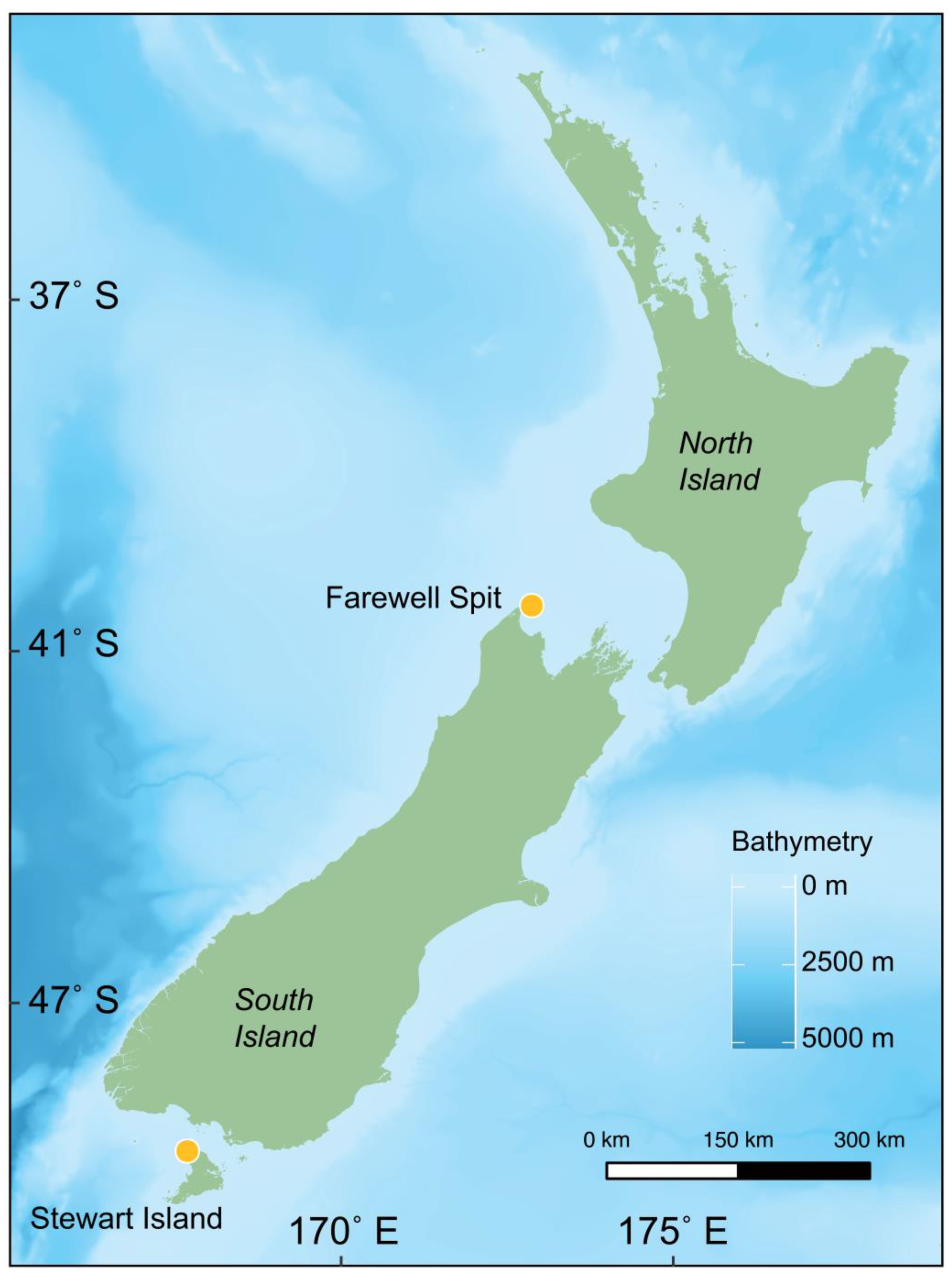
To assess isotopic profiles of G. m. edwardii in New Zealand waters, archived skin samples (n = 125) were analysed from individuals collected from stranding events between 2009 and 2017 (summarised in Supplementary Material Table S1).

2.1. Sampling

Skin was sampled from six stranding events across two G. m. edwardii stranding hotspot locations in New Zealand; Onetahua Farewell Spit (FWS; −40.481° S, 172.870° E) and Rakiura Stewart Island (SI; −46.686° S, 167.685° E; [50]; see Figure 1). Of these, 87 carcasses were sampled at FWS during four mass-stranding events (2009, 2011, 2014, 2017) and 38 carcasses at SI during two mass-stranding events (2010, 2011). All of the mass-strandings sampled occurred during the austral summer between the months of November and February.

Skin sampling, along with measurements of body length and an anatomical assessment of sex, was undertaken in situ at stranding events using standard postmortem procedures [58]. All skin samples were stored at 4 °C in 70% ethanol prior to analysis. Teeth and reproductive organs were sampled where possible, as outlined in [59], with age data available for 86% (108 of 125) of individuals and reproductive data available for 82% (102 of 125) individuals. Teeth were used to assess age via dentinal growth layer groups [59]. Reproductive organs were used to assess sexual maturity status (herein referred to as maturity status) and reproductive group for mature females, where possible [60,61]. Six reproductive groups were defined: immature males, mature males, immature females, pregnant females, lactating females, and resting females. Male maturity was defined by presence/absence of sperm in testes [61]. Females were defined as “pregnant” by the presence/absence of a foetus, as “lactating” by presence/absence of milk in the mammary glands, and as “resting” by the presence of ovarian corpora indicating previous ovulation, but with no foetus or milk present [60]. However, if reproductive group and/or maturity status were not available, body length was used as an indicator of maturity status using estimations from the same G. m. edwardii population [60,61]. Where sample availability allowed, samples were compared in equal groups of mature males (n = 5), mature females (n = 5), immature males (n = 5) and immature females (n = 5) within each stranding event. In one stranding event (FWS2014), more mature females of known reproductive group were available, and these were therefore included in analyses to increase comparative statistical power of mature female reproductive groups (

Table 1. Ontogenetic characteristics of long-finned pilot whales (Globicephala melas edwardii) sampled for stable isotope analysis from mass-strandings on the New Zealand coast, 2009–2017. Unknown refers to individuals where reproductive group was unable to be determined from reproductive organs, but maturity status was instead classified from body length.

Ontogenetic Status	n	Body Length Range (cm)	Age Range (Years)
Maturity status
Immature	56	168–482	0–13
Mature	69	364–595	6–33
Reproductive group
Immature male	26	255–482	1–13
Mature male	18	467–581	14–31
Immature female	25	168–375	0–8
Pregnant female	17	364–461	6–33
Lactating female	9	380–446	7–30
Resting female	7	397–453	11–30
Unknown	23	194–595	5–32

).

Carbon and nitrogen stable isotopes from skin samples (n = 125) were analysed to compare ontogenetic and spatiotemporal variation. Additionally, a subset of 36 (13 male and 23 female) samples from sexually mature individuals with the highest, lowest, and median carbon and nitrogen isotope values recorded per stranding event were analysed for sulphur isotope values. Immature individuals excluded from analyses of sulphur isotopes to avoid confounding the data with individuals that were not fully weaned.

2.2. Sample Preparation

In preparation for stable isotope analysis, skin samples were placed under the fume hood for at least 48 h [62] to evaporate off the storage ethanol. Samples with excess ethanol remaining were further placed under a stream of nitrogen gas until all ethanol had been removed from the sample. Samples were cut longitudinally to capture all skin layers, as recommended for isotopic studies of cetaceans aiming to consider trophic interactions and diet composition [63]. Skin was then homogenized by finely slicing in a glass Petri dish using a clean scalpel blade. Approximately 40 mg of each sample was weighed into Eppendorf tubes and freeze-dried overnight for a minimum of 18 h or dried in an oven at 60 °C for at least 48 h.

2.3. Carbon and Nitrogen Isotope Analysis

Carbon and nitrogen isotope analysis was carried out at the Environmental and Ecological Stable Isotope Analytical Facility at the National Institute for Water and Atmospheric Research (NIWA), Wellington. Around 1.0 mg of each homogenised skin sample was weighed into tin capsules using a six decimal place (g) microbalance. Tin capsules were formed into balls containing the sample and were analysed by a FLASH 2000 elemental analyser with MAS 200 R autosampler linked to a DELTA V Plus continuous flow isotope ratio mass spectrometer (Thermo Fisher Scientific, Bremen, Germany). Stable isotope values were calculated using ISODAT (Thermo Fisher Scientific) software; δ¹³C values were calibrated against Carrara Marble NSB-19 (National Institute of Standards and Technology (NIST), Gaithersburg, MD, USA) and δ¹⁵N relative to Pee Dee Beleminte (PDB) standard followed by correction for O¹⁷. International laboratory reference materials from NIST were run at the start and end of eve ry batch of analyses for data normalisation [64]. A working laboratory standard of DL-Leucine (DL-2-Amino-4-methylpentanoic acid, C6H13NO2, Lot 127H1084, Sigma, Melbourne, Australia) and squid were run every 10 samples to correct for machine drift, for quality control and to report on precision. The international standards USGS65 Glycine was also run every ten samples to check accuracy and precision. Data accuracy was measured to better than 0.15‰ for δ¹³C and δ¹⁵N values, whilst precision was measured to better than 0.24‰ for δ¹³C and 0.22‰ for δ¹⁵N values. Stable isotope ratios were expressed as delta values (δ) in per mil units (‰), which represent the ratios of heavy to light isotopes within a sample (R_sample), relative to the ratio in an international standard (R_standard) as:

$$\mathsf{\delta }=\left(\left(\frac{{\mathrm{R}}_{\mathrm{sample}}}{{\mathrm{R}}_{\mathrm{standard}}}\right)-1\right)\times 1000$$

2.4. Sulphur Analysis

A subset of 36 skin samples from mature individuals was processed for sulphur isotope analysis at IsoTrace Limited, Dunedin. Samples were analysed using the Carlo Erba NC 2500 elemental analyser coupled to a Europa Hydra isotope ratio mass spectrometer. Stable isotope values were normalised against international standards of Vienna PDB, AIR and Canyon Diablo Troilite for carbon, nitrogen, and sulphur, respectively. Two international reference materials comprising USGS40 mixed with IAEA-S1 (carbon = −26.39‰, nitrogen = −4.52‰, sulphur = −0.30‰), and USGS-41 mixed with IAEA-S2 (carbon = 36.55‰, nitrogen = 47.55‰, sulphur = 22.62‰) used for data normalisation in a three-point system. Replicate analysis of the keratin internal working laboratory standard was used to determine machine drift, and precision of ẟ¹³C (0.08‰), ẟ¹⁵N (0.04‰) and ẟ³⁴S (0.16‰) was assessed from replicates positioned every ten samples.

2.5. Correction Equations

Lipids are depleted in ¹³C relative to ¹²C compared to proteins. The lipid content of ecological samples therefore affects δ¹³C values [65]. Lipids are thus either removed from the sample before carbon stable isotope analysis, e.g., [17,66,67,68] or a lipid correction equation is applied to samples with C:N mass ratios > 3.5 to correct for the lipid-affected δ¹³C values [69,70,71]. There is disagreement within published literature regarding the suitability of lipid correction equations being extrapolated to different species for isotopic studies [72]. Therefore, lipids were extracted from a sub-set of ten G. m. edwardii skin samples (Supplementary Material Table S2) to check the validity of using published lipid correction equations [69,73,74,75]. Samples were selected from one location only (FWS) based on, (1) extreme carbon and nitrogen isotope values in comparison to the rest of the dataset and, (2) a wide range of C:N mass ratios. Selected samples had C:N mass ratios ranging from 3.27–4.48 and C:N atomic ratios ranging from 3.81–5.23. The lipid correction equation, which was based on a bootstrapping approach using 74 samples of odontocetes, including G. m. edwardii from Peters et al. [75], was found to be the best fit for the data. The lipid correction equation:

δ¹³C_corrected = 0.5301486 × δ¹³C − 7.322335

was applied to δ¹³C values for samples with a C:N mass ratio over 3.5. Bulk isotope uncorrected δ¹³C values were used when C:N mass ratios were <3.5. As lipid extraction can affect nitrogen and sulphur isotope values [76], non-lipid extracted bulk samples were analysed to generate ẟ¹⁵N and ẟ³⁴S values. Additionally, to account for changing carbon dioxide levels in the ocean due to anthropogenic activity [77], commonly referred to as the Suess effect, a correction equation of −0.022% y⁻¹ [78] was applied to all δ¹³C values to the baseline of our most recent sample set collected in 2017.

2.6. Statistical Analysis

Following testing assumptions of normality using Shapiro–Wilk tests, Kruskal–Wallis tests were used in the R package “rstatix” [79] to compare differences in mean ($\overline{x}$) δ¹³C, δ¹⁵N and δ³⁴S values both within and among groups defined as: sex, reproductive group, stranding location, stranding event, and stranding year. For δ¹³C and δ¹⁵N values, these were also compared among maturity status, which was not an option for δ³⁴S as we only had δ³⁴S values for mature animals. Where significant differences occurred, pairwise data were compared using Wilcoxon tests to determine differences between specific groups, e.g., [17,80]. Spearman’s correlation coefficient was used to determine if any relationship occurred between body length or age and δ¹³C, δ¹⁵N and δ³⁴S values, respectively. The relationship between δ¹³C, δ¹⁵N, and δ³⁴S values and a suite of predictive variables was investigated using generalised additive models (GAMs) [81] using the R package “mgcv” [82]. Predictive variables were sex, body length, maturity status (only for δ¹³C and δ¹⁵N values), stranding location, stranding event and stranding year. Body length was fitted as a continuous variable, whereas sex, maturity status, stranding location, stranding event and stranding year were fitted as factors. As body length and age were highly correlated (Spearman rank, rho = 0.85, p ≤ 0.01), and age was not available for all individuals, body length (n = 125) was included in GAM models as a proxy rather than age itself (n = 108). Models were built with Gaussian distribution with gamma set to 1.4 to prevent overfitting [83] with all possible combinations of variables. Akaike’s information criterion adjusted for small sample size (AICc; [84]) was using the R package “qpcR” [85] to select the best fitting model. Interactions for the five top-ranked models were also tested. Final models were checked for normality and obvious patterns in the residuals. Niche partitioning was investigated using Bayesian inference using the R packages “SIBER” [27] and “ggplot2” [86] with ellipses calculated at the 0.40 and 0.95 α level.

Niche regions (NR) were presented in three-dimensions (‰³) using δ¹³C, δ¹⁵N and δ³⁴S data using the R packages “scatterplot3d” [87] and “nicheROVER” [88]. Volume of ellipses was set at the 0.40 α level (NR₄₀, e.g., [10]). Data were split into groups based on ontogenetic variation and stranding event to calculate pairwise isotopic niche overlap. For ontogenetic variation, data were classified as mature males, mature females, and pregnant/lactating females due to data availability. Published methods were followed [89], replacing “Species” with “Group”, whereby pairwise niche overlap was defined as the probability (%) of an individual from one group being found within the NR₄₀ of another group. Data were presented as a pairwise grid of one-dimensional isotopic density distributions, two-dimensional pairwise isotopic scatter plots and two-dimensional NR₄₀ ellipses of five random NR₄₀ estimates. Overlap probability was calculated at the 95% level using a Bayesian approach with 10,000 iterations and reported as mean posterior overlap, e.g., [10].

The relationship between number of G. m. edwardii stranded and triple isotope niche size was examined through Pearson’s correlation analysis both with and without FWS2009 data included. The FWS2009 stranding event appeared anomalous as it had a much larger niche size for the number of animals stranded compared to all other events, and did not fit the trend of the other stranding events. Finally, isotopic range of δ¹³C using the highest and lowest values were calculated using the formula:

$${∆}_y={\delta }^{13}{C}_{ymax}-{\delta }^{13}{C}_{ymin}$$

where $y$ = sample size [90]. Isotopic ranges of δ¹⁵N and δ³⁴S were calculated in the same way at the level of (1) the entire dataset, and (2) each stranding event.

All data analysis was completed in R version 4.0.5 [91].

3. Results

Lipid corrections were performed on δ¹³C values from 71 (57%) samples, whilst 54 samples (43%) were not lipid-corrected (Supplementary Material Table S3). Following δ¹³C corrections for lipid content and Suess effects, δ¹³C data were not normally distributed (Shapiro–Wilk, W = 0.96, p = 0.001). Overall, neither δ¹⁵N values (Shapiro–Wilk, W = 0.83, p ≤ 0.05) nor δ³⁴S values (Shapiro–Wilk, W = 0.94, p = 0.03) were normally distributed.

3.1. Ontogenetic Variation in δ¹³C, δ¹⁵N and δ³⁴S Values

The mean δ¹⁵N value was 12.59 ± 0.72‰ (

Table 2. Range, mean and standard deviations (±1 SD) of carbon and nitrogen (δ¹³C and δ¹⁵N) values of long-finned pilot whales (Globicephala melas edwardii) stranded on the New Zealand coast, 2009–2017, presented by sexual maturity status and reproductive group. Unknown refers to individuals where reproductive group was unable to be determined from reproductive organs, but maturity status was instead classified from body length.

		δ13C (‰)			δ15N (‰)
	n	Range	Mean	SD	Range	Mean	SD
All	125	−18.80 to −15.53	−17.12	0.73	11.52 to 16.28	12.59	0.72
Maturity status
Immature	56	−18.80 to −15.53	−17.00	0.70	11.90 to 15.23	12.59	0.58
Mature	69	−18.77 to −15.82	−17.23	0.74	11.52 to 16.28	12.60	0.82
Reproductive group
Immature male	26	−18.16 to −16.26	−16.79	0.52	11.97 to 13.27	12.38	0.30
Mature male	18	−18.77 to −16.26	−17.00	0.69	11.52 to 13.27	12.34	0.53
Immature female	25	−18.80 to −15.53	−17.12	0.81	11.90 to 13.93	12.64	0.53
Pregnant female	17	−18.32 to −16.02	−17.13	0.73	11.83 to 14.85	12.53	0.72
Lactating female	9	−18.59 to −16.39	−17.40	0.71	11.70 to 12.85	12.30	0.42
Resting female	7	−18.74 to −15.82	−17.59	1.01	11.72 to 13.37	12.34	0.60
Unknown	23	−18.62 to −15.99	−17.26	0.68	11.75 to 16.28	13.23	1.10

), whilst the mean δ¹³C value was −17.12 ± 0.73‰ (n = 125). No significant correlations were found between δ¹³C values and body length (Spearman rank, rho = −0.06, p = 0.54) nor age (Spearman rank, rho = −0.12, p = 0.22), respectively. Futher, no significant differences were found in the δ¹³C values between males (−17.04 ± 0.65‰, n = 57) and females (−17.20 ± 0.79‰, n = 68; Kruskal–Wallis, ts = 0.98, p = 0.32, Figure 2), between immature (−17.00 ± 0.70‰, n = 56) and mature (−17.23 ± 0.74‰, n = 69) individuals (Kruskal–Wallis, ts = 2.89, p = 0.09) or among reproductive groups (immature males: −16.79 ± 0.81‰, n = 26; mature males: −17.00 ± 0.69‰, n = 18; immature females −17.12 ± 0.81‰, n = 25; pregnant females: −17.13 ± 0.73‰, n = 17; lactating females: −17.40 ± 0.71‰, n = 9; resting females: −17.59 ± 1.01‰, n = 7; Kruskal–Wallis, ts = 9.06, p = 0.11, Table 2, Figure 3).

Similarly, no significant correlations were found between δ¹⁵N and body length (Spearman rank, rho = −0.08, p = 0.36) nor age (Spearman rank, rho = −0.09, p = 0.37), respectively. No differences in the δ¹⁵N values between males (12.62 ± 0.70‰, n = 58) and females (12.57 ± 0.75‰, n = 67, Kruskal–Wallis, ts = 0.41, p = 0.52), between immature (12.59 ± 0.58‰, n = 56) and mature individuals (12.60 ± 0.82‰, n = 69, Kruskal–Wallis, ts = 0.53, p = 0.47) or among reproductive groups (immature males: 12.38 ± 0.30‰, n = 26; mature males: 12.34 ± 0.53‰, n = 18; immature females 12.64 ± 0.53‰, n = 25; pregnant females: 12.53 ± 0.72‰, n = 17; lactating females: 12.30 ± 0.42‰, n = 9; resting females: 12.34 ± 0.60‰, n = 7; Kruskal–Wallis, ts = 6.14, p = 0.29) were detected (Table 2).

The mean δ³⁴S value was 21.42 ± 0.91‰ for the pooled dataset (n = 36). Sulphur isotope values did not differ significantly between sex (males 21.14 ± 0.99, n = 13; females 21.58 ± 0.83, n = 23; Kruskal–Wallis, ts = 1.87, p = 0.17,

Table 3. Mean and standard deviations (±1 SD) of carbon, nitrogen, and sulphur (δ¹³C, δ¹⁵N and δ³⁴S) values of a subset of 36 mature long-finned pilot whales (Globicephala melas edwardii) stranded on the New Zealand coast (2009–2017), presented by sex and reproductive group.

		δ13C (‰)		δ15N (‰)		δ34S (‰)
	n	Mean	SD	Mean	SD	Mean	SD
Male	13	−17.32	0.81	12.59	0.72	21.14	0.99
Female	23	−17.06	0.82	12.70	1.04	21.58	0.83
Pregnant/Lactating female	14	−17.12	0.73	12.68	0.75	21.56	0.90
All	36	−17.14	0.78	12.66	0.93	21.42	0.91

). Similarly, no significant correlations were found between δ³⁴S and age (Spearman rank, rho = −0.20, p = 0.27) nor body length (Spearman rank, rho = −0.21, p = 0.22).

3.2. Spatial and Temporal Variation in δ¹³C, δ¹⁵N and δ³⁴S Values

Overall, individuals that stranded at FWS (n = 87) had significantly lower δ¹³C and higher δ¹⁵N values (δ¹³C—17.39 ± 0.68‰, δ¹⁵N 12.71 ± 0.79‰) compared to those stranded at SI (δ¹³C—16.51 ± 0.39‰, n = 38; Kruskal–Wallis, ts = 45.6, p ≤ 0.01; δ¹⁵N 12.32 ± 0.44‰, Kruskal–Wallis, ts = 8.43, p ≤ 0.01, Figure 4). Total niche area (TA) and corrected standard ellipse areas (SEA_C) were larger for females at both FWS (female TA = 7.64, SEA_C = 1.89, n = 47; male TA = 4.72, SEA_C = 1.25, n = 40) and SI (female TA = 2.74, SEA_C = 0.79, n = 20; male TA = 0.83, SEA_C = 0.28, n = 18). The TA and SEAc values were larger at FWS than SI for both males and females, respectively. The TA was largest for pregnant females at FWS (TA = 3.14, SEA_C = 1.96, n = 10), and smallest for mature males at SI (TA = 0.30, SEA_C = 0.27, n = 7; Supplementary Material Table S4).

Differences in δ¹³C were recorded between stranding events (Kruskal–Wallis, ts = 89.7, p =< 0.01), with Wilcoxon tests describing four pairs as not significantly different: FWS2014, FWS2017 (p = 0.40); and FWS2009, SI2010 (p = 1); FWS2009, SI2011 (p = 0.25) and SI2010, SI2011 (p = 0.25). Mean δ¹³C values were lowest in FWS2017 stranded individuals ($\overline{x}$ = −18.04 ± 0.52‰, n = 20), whereas the highest mean δ¹³C values were observed in those stranded at FWS2009 ($\overline{x}$ = −16.65 ± 0.31‰, n = 20). Nitrogen isotope values differed among stranding events (Kruskal–Wallis, ts = 57.1, p ≤ 0.01), with higher δ¹⁵N values recorded in individuals from FWS2017 (n = 20) than any other stranding event. Nitrogen isotope values were also lower at the FWS2014 stranding event (n = 27) than any other FWS stranding event.

Sulphur isotope values did not differ significantly between stranding events (Kruskal–Wallis, ts = 9.24, p = 0.10) nor stranding location (FWS: 21.33 ± 0.95‰, n = 32; SI: 21.61 ± 0.82‰, n = 18; Kruskal–Wallis, ts = 0.65, p = 0.42; Figure 5).

The top three GAMs for δ¹⁵N retained only stranding event, location, and year. The top model retained only stranding event as a covariate, explaining 45% of the deviance (

Table 4. Summary statistics for the top three generalised additive models (GAMs) selected based on Akaike Information Criterion corrected for small samples sizes (AICc) of long-finned pilot whale (Globicephala melas edwardii) skin samples, presented by carbon, nitrogen and sulphur (δ¹⁵N, δ¹³C and δ³⁴S) values. LL: log-likelihood; % DE: % deviance explained; ΔAICc: difference in Akaike’s information criterion (AIC_C) of the current and top-ranked model; wAICc = AIC_C weight. Significant variables are highlighted in bold.

Model	R2	LL	% DE	∆AICc	wAICc
δ15N
Stranding event	0.431	1.000	45.40	-	0.145
Location + Stranding event	0.431	0.885	45.40	0.250	0.128
Year + Location	0.425	0.553	44.90	1.190	0.080
δ13C
Maturity + Stranding event	0.679	1.000	69.40	-	0.119
Maturity + Year + Location	0.679	1.000	69.40	-	0.119
Sex + Maturity + Year + Location	0.680	0.87	69.80	0.284	0.103
δ34S
Sex	0.030	1.000	5.59	-	0.211
Year	0.020	0.885	4.77	0.250	0.186
Location	0.030	0.486	8.85	1.440	0.102

). For δ¹³C values, the top two best-fit models retained maturity status, location, year and stranding event as covariates and explained 69% of the deviance. Sex stranding event was also retained as a covariate in the top three GAMs fitted for δ¹³C data (Table 4). Whilst body length was also fitted to GAMs, this was not retained in the top-ranked models. The top-ranked GAM for δ³⁴S retained only sex as a covariate. Stranding location and year were also retained, respectively, as covariates in the top three models (Table 4). However, the deviation explained was less than 10% for all models (Table 4), indicating that the included predictor variables did not explain the data well.

3.3. Triple Isotope Niche Regions

Triple isotope niche regions at the α = 40 level (NR₄₀) were calculated by ontogenetic variation and stranding event. Pairwise comparisons showed the NR₄₀ overlaps of individuals from differing ontogenetic groups (

Table 5. Confusion matrices of triple isotope (δ¹³C, δ¹⁵N and δ³⁴S) niche overlap at the 95% confidence level of mature long-finned pilot whales (Globicephala melas edwardii) processed from stranding events on the New Zealand coast between 2009 and 2017. Values are the chances (%) that an individual from the group on the left-hand column would be found within isotope niche of any of the other groups in its row. Data presented by (a) maturity status and (b) stranding event.

(a)
		Mature Male		Mature Female		Pregnant/Lactating Female
Male				82.14		75.73
Female		48.41				74.90
Pregnant/Lactating female		57.30		91.45
(b)
	FWS2009	FWS2011	FWS2014		FWS2017	SI2010	SI2011
FWS2009		21.05	2.65		0.86	25.02	21.11
FWS2011	36.13		17.57		4.07	5.81	27.04
FWS2014	7.94	26.35			9.61	0.38	8.16
FWS2017	1.49	3.51	2.48			0.00	0.75
SI2010	74.78	20.34	1.09		0.01		41.57
SI2011	58.80	29.13	7.26		0.76	37.41

a). Females had the most unique isotopic niche space, with only a 48% chance any resting females would be found in the NR₄₀ of mature males but a 75% chance they would be found in the NR₄₀ of pregnant/lactating females (Table 5a). However, there was a high degree of probability that both mature males (82%) or pregnant/lactating females (91%) would be found within the NR₄₀ of all females. Likewise, mean niche size was much larger for all females (mean ± SE = 53.58 ± 13.82‰³) than either pregnant/lactating females (33.56 ± 11.24‰³) or males (20.72 ± 7.18‰³). Mean niche size was similar across several stranding events; FWS2011 (6.62 ± 3.60‰³), FWS2014 (4.32 ± 2.27‰³), SI2011 (4.11 ± 2.21‰³) and SI2010 (3.78 ± 2.04‰³). The combined niche width of individuals stranded at FWS2009 (17.62 ± 9.42‰³) and FWS2017 (15.52 ± 8.25‰³) were much larger than those of all other stranding events (Figure 6).

There was a 59% chance of an individual from SI2011 being found in the NR₄₀ of FWS2009, the highest probability recorded. However, there was only a 1% chance of an individual from FWS2017 being found within the NR₄₀ of SI2010. Individuals stranded at FWS had a 0–36% chance of being found in the NR₄₀ of individuals stranded at SI, whereas there was a much higher chance (0–75%) of an individual from SI being found in the NR₄₀ of an individual stranded at FWS. Several pairs were considered to have low probability of NR₄₀ overlap (<10%), with individuals from FWS2017 seemingly the least likely to be detected within the NR₄₀ of any other stranding event (Table 5b). The NR₄₀ overlap appeared high both between stranding events occurring at the same site (e.g., SI2010 and SI2011) and those that were temporally close (e.g., FWS2009 and SI2010 which occurred only three months apart, Table 5b).

No significant correlation between stranding group size and niche size (correlation = 0.55, p = 0.26) was detected. However, when the FWS2009 stranding event was removed from the dataset, a significant positive correlation was revealed between the number of animals involved in the stranding event and the niche width (correlation = 0.92, p = 0.03). Finally, isotopic range was found to be similar between δ¹³C (3.27‰), δ¹⁵N (4.75‰) and δ³⁴S (4.30‰) values for the entire pooled dataset (

Table 6. Isotopic range expressed as a percentage of carbon, nitrogen, and sulphur (δ¹³C, δ¹⁵N and δ³⁴S) values of long-finned pilot whales (Globicephala melas edwardii) sampled from mass-stranding events on the New Zealand coast, 2009–2017. Data are presented by overall dataset, and by each stranding event: FWS = Farewell Spit, SI = Stewart Island.

Isotope Range (‰)	Overall	FWS2009	FWS2011	FWS2014	FWS2017	SI2010	SI2011
n	125	20	20	27	20	19	19
δ13C	3.27	1.15	0.96	1.64	1.58	0.76	1.90
δ 15N	4.76	2.95	1.96	1.47	3.85	2.18	1.86
n	36	6	6	6	6	6	6
δ34S	4.30	2.24	2.72	1.15	2.80	3.27	1.18

). The smallest range of δ¹³C values were found at the SI2010 stranding event (0.76‰) along with the largest range of δ³⁴S values (3.27‰). In contrast, the largest range of δ¹³C values were recorded at the SI2011 stranding event (1.90‰) and the smallest range of δ³⁴S values (1.15‰) were recorded at FWS2014. Finally, the largest range of δ¹⁵N values were recorded at the FWS2017 (3.85‰) stranding event, whereas the smallest range was at the FWS2011 stranding (1.20‰).

4. Discussion

Intraspecific variation in isotopic values has been explored in multiple cetacean species [1]. Here, we analysed ontogenetic and spatiotemporal effects on the isotopic niche of a single cetacean species, G. m. edwardii. Overall, isotopic data from this study were characterised by a high level of overlap between the 125 individuals analysed for δ¹³C and δ¹⁵N and the 36 individuals analysed for δ³⁴S. Significant differences were found in both δ¹³C and δ¹⁵N, but not δ³⁴S values when examined by location stranded and stranding event. No significant differences were found in δ¹³C, δ¹⁵N and δ³⁴S values vs. sex, body length, age, maturity status or reproductive group.

In general, mean δ¹⁵N values for G. m. edwardii reported in this study ($\overline{x}=$ 12.71‰, n = 125) were lower than mean values reported for other cetacea in New Zealand waters around the same time period, e.g., teuthophagus common dolphins Delphinus delphis (female $\overline{x}=$ 14.88‰, n = 33; male $\overline{x}=$ 14.81‰, n = 23; [92]) and male sperm whales Physeter macrocephalus ($\overline{x}=$ 15.6‰, n = 37; [93]). However, mean δ¹⁵N values were still higher than other New Zealand marine mammals with diets that are more focused on copepods and krill, such as blue whales Balaenoptera musculus sp. ($\overline{x}=$ 11.1‰, n = 8; [94]) and southern right whales Eubalaena australis ($\overline{x}=$ 8.09‰, n = 18; [95]). Lower δ¹⁵N values were also recorded in G. m. melas in the Mediterranean in comparison to other teuthophagus odontocetes such as P. macrocephalus and Risso’s dolphins Grampus griseus [35]. This could be indicative of offshore feeding [96,97,98]. Indeed, δ¹⁵N values reported in this study were consistent with those of other G. melas populations globally [37,47,99,100,101]. Similarly, δ¹³C values recorded here were comparable to those measured in northern hemisphere G. m. melas populations [47,102,103].

Sulphur isotopes can provide useful information on foraging prey source pathways [20,21], G. m. edwardii δ³⁴S values from this study were similar to those reported in G. m. melas in the Mediterranean [102]. High δ³⁴S ($\overline{x}=$ 21.52‰, n = 36) values indicated a large contribution to diet from marine sulphate, indicating marine foraging pathways [20,104,105]. The combination of low δ¹³C values with high δ³⁴S values observed in this study has previously been described as typical of oceanic feeding behaviour [106], corroborating that G. melas is primarily an oceanic species [34,107,108].

4.1. Ontogenetic Variation in Isotope Values

No observable differences in isotopic niche among the different ontogenetic groups were detected in this study, aligning with observed isotopic homogeneity of G. m. melas in the Strait of Gibraltar [37]. Whilst sex differences in resource-use have been reported in other cetacean species including bottlenose dolphins T. truncatus [109], this has not been recorded in G. melas previously. Furthermore, higher cadmium levels have been reported in female G. m. edwardii from New Zealand waters than in males [110]. Higher cadmium load in females could signify a greater reliance on cephalopod prey [111], as cephalopods are known to accumulate cadmium in their tissues [112]. Females had a larger TA than males when considering only δ¹³C and δ¹⁵N values and were less likely to be found in the triple isotope niche of males (56%) than the other way around (79%, Table 5a). Yet, no differences were detected in mean δ¹³C, δ¹⁵N or δ³⁴S values between males and females. Whilst sex was retained as a predictor in the top-ranked GAM for δ³⁴S (Table 4), the deviance explained was very low (6%), indicating that there are likely other factors that determine δ³⁴S values.

Like many cetacean species, G. m. edwardii displays sexual dimorphism with males being larger than their female counterparts [60,113]. It is possible that increased overall body size, rather than sex, could be driving the small isotopic niche differences reported here. However, body length was not retained as a predictor in the top-ranked models for δ¹³C, δ¹⁵N or δ³⁴S (Table 4) nor significantly correlated with isotopic values. Whilst maturity status was retained as a predictor explaining δ¹³C variation, this was not the case for δ¹⁵N or δ³⁴S data. Hence, this study did not reveal a link between consumption of prey from higher trophic levels and body length. Similarly, no relationship was evident between stable isotope values and body length in P. macrocephalus [93,114], or δ³⁴S, sex and body size in T. truncatus [104].

An increased reliance on higher trophic levels with increased body length has been reported in weaned striped dolphins Stenella coeruleoalba [42,115], whilst studies of P. macrocephalus, Commerson’s dolphins Cephalorhynchus commersonii commersonii, common dolphins D. capensis and T. truncatus all reported an increase in δ¹⁵N with age [9,38,44,116]. Though no statistical relationship was apparent between isotope values and body length or age in this dataset, high δ¹⁵N values were recorded in some of the smallest and youngest pilot whales, which is consistent with reliance on lactation in young cetacea [68,117,118].

The effect of reproduction on stable isotope values in cetaceans has not been as well studied, but it has been suggested that energetic demands and nutrient intake of mature females can differ due to reproductive status [119,120,121]. In this study, pregnant females had the largest isotopic niche of all reproductive groups. It has been suggested that the specific stage of pregnancy could affect isotope values of humpback whales Megaptera novaeangliae [122], so further distinction in reproductive groups, including pregnancy stage, may be necessary to elucidate isotopic variability. Furthermore, lactating G. m. edwardii often had higher δ¹⁵N values than resting females, though this difference was not statistically significant. In general, older females that are no longer reproductively active may target riskier prey [123], causing a change to their isotopic niche. However, resting G. m. edwardii in this study were not necessarily of advanced age. Overall, isotopic homogeneity among reproductive groups could be due to trophic similarity within the population, lack of sufficient samples within each stranding event or indeed, varying stages of pregnancy. A similar lack of variation in isotope values by reproductive group has been reported in sei whales, B. borealis and Bryde’s whales, B. edeni [124]. Differences in isotopic values that do not meet the threshold for statistical significance have been previously proven ecologically significant through the use of complementary dietary analysis methods such as fatty acid analysis [125]. Accordingly, future examination of fatty acid profiles for the New Zealand G. m. edwardii population could shed further light on their foraging ecology.

4.2. Spatial and Temporal Variation in Stable Isotope Values

Spatial differences in isotopic composition within a population are well recorded in cetacea, including G. melas [47,100]. For example, spatial differences in δ¹⁵N values have been attributed to prey selection and trophic breadth, whilst differences in δ¹³C have been linked to feeding area (e.g., offshore or coastal) and latitude [1,8]. It was predicted that SI strandings events would have lower δ¹³C values compared to FWS due to the more southerly location [126], however the opposite was true (Figure 4). Furthermore, δ¹⁵N values were consistently lower in SI than FWS. The lack of significant differences in sulphur isotope values suggests that these carbon and nitrogen isotopic variances are likely due to variation in primary productivity and baseline isotope values between the two locations rather than differences in diet or food web pathways. Future studies would benefit from baseline isotopic information obtained from either: (1) sampling suspended particulate organic matter in surface waters or a sessile primary consumer; or (2) employing compound specific isotope analysis to tease out confounding baseline versus trophic level drivers of elevated ẟ¹⁵N values [127,128,129,130].

The isotopic ranges of values per stranding event for carbon, nitrogen and sulphur were much smaller than those observed in the overall dataset. Furthermore, stranding event was retained in three of the top six GAMs reported for ẟ¹³C and ẟ¹⁵N, indicating that stranding event was an important driver of variation for carbon and nitrogen isotopic values. Individuals involved in the SI2010 mass-stranding had the smallest niche size of all the stranding events, which indicates little inter-individual difference in prey and foraging locations for animals involved in this stranding event. However, SI2010 was also the event with the smallest number of overall individuals stranded (Table S1) which may confound the results. The widest NR₄₀ was recorded at FWS2009 even though this stranding did not comprise the most animals stranded. When FWS2009 was removed from the dataset, a positive correlation was seen between niche size and the total number of G. m. edwardii from all other stranding events. Although long-finned pilot whales are generally believed to live in matrilineal pods [131,132], mass-stranding events of G. m. edwardii on the New Zealand coast have been reported to involve individuals from many different maternal lineages [133]. This wider NR₄₀ and isotopic variability could therefore signify multiple groups that have previously been dispersed from each other [134], but have fused to form a “super pod” shortly prior to stranding. With little other information available, such as genetic barcoding for individuals within stranding events, it is impossible to assume the genetic or social composition of the FWS2009 stranding event. It could be that the individuals stranded in FWS2009 represented a single pod. If that were the case, a wide NR could indicate a more heterogeneous feeding strategy or utilisation of more varied resources [135]. Both a wide isotopic niche and heterogeneity of isotopic niche within a population can indicate a generalist feeding strategy, diversified diet, or a degree of individual dietary specialization [136,137,138].

The large niche size recorded in FWS2009 appeared to be driven by a larger range of δ¹⁵N values compared to other stranding events (Table 6). The individuals stranded in the FWS2017 event also recorded a large niche size, driven by both the largest range of δ¹⁵N values and second largest range of δ³⁴S values compared to other stranding events (Table 6). This indicates that individuals in these two stranding events had a more varied diet. This could be due to ingestion of a mixture of different trophic level prey which themselves feed in a variety of benthic/pelagic, and coastal/oceanic habitats. Isotopic density plots for both FWS2011 and SI2010 (Figure 6) also had lower δ³⁴S values, suggesting an inshore or benthic component to feeding prior to these stranding events [20,139]. Globally, G. melas have been recorded as having dietary plasticity, displaying behavioural changes by following prey that have migrated due to changes in oceanic currents and water temperatures and adapting their diet to locally available prey [49,140]. Indeed, observations of a single captive G. m. melas showed a preference shift to the more abundant prey when prey proportions were varied [141]. Stomach content studies of G. m. edwardii from New Zealand waters suggest a large dietary reliance on arrow squid Nototodarus spp. [51,52,53].

It is difficult to ascertain whether changes such as a widening NR₄₀ are indicative of a temporal niche change since the data in this study only span a few years. Whilst δ¹⁵N values were highest in 2009 they were also high in 2017, suggesting there is not a linear temporal pattern in δ¹⁵N values. However, a temporal decline in δ¹³C values at FWS was noted between 2009 and 2017 (Figure 6), echoing similar findings from marine predators such as tuna (Tunnus albacares, T. obesus and T. alalunga; [142]) and D. delphis [92] across the Pacific Ocean in recent years. Whilst seasonal differences in prey have been recorded in G. m. melas population in the northern hemisphere [37,48], data in this study are exclusively from mass-strandings that occurred during the austral summer (November to February) in New Zealand [50], preventing seasonal comparisons.

Resource partitioning of socially and spatially distinct groups has been noted in other cetacea [115,143]. Although stranding records and sightings data show that G. m. edwardii strand all around New Zealand, only two stranding hotspot locations [50] were explored here. Despite the geographic separation of SI and FWS (800 km apart) there was little isotopic variability between stranding events at the two locations when strandings occurred within the same year. In the absence of tracking, genetic, or migratory data, it is not known whether any surviving members of the FWS2009 stranded pod were involved in the stranding event three months later at SI.

Population homogeneity has been recorded in northern hemisphere G. m. melas populations [144], suggesting that individuals in the same pods may feed in similar environments. As stranding event appeared to be the most prominent predictor of niche, a degree of individual/group specialisation [37] or cooperative foraging may exist, as has been observed in other odontocetes [145]. Multiple feeding techniques have been observed in G. melas populations, including both shallow and deep foraging dives [146,147] and nocturnal [148,149] and suction feeding [150] in captive animals. Satellite tagging of the closely related short-finned pilot whales G. macrorhynchus in the northeastern Atlantic revealed that individuals may be able to adapt foraging states and behaviour per dive in response to immediate physiological and environmental constraints [151]. However, it is not clear what foraging strategy G. m. edwardii utilise in New Zealand waters due to a lack of tagging, video, or distribution data for this species.

5. Conclusions

This study was the first to investigate isotopic variation of G. m. edwardii in New Zealand waters. Overall, spatiotemporal variation appeared to have a greater effect on isotopic values than ontogenetic variation, with significant differences in δ¹³C and δ¹⁵N values detected between stranding location and event. Whilst δ³⁴S values did not directly relate to ontogenetic or spatiotemporal factors, incorporating sulphur isotope data improved isotopic niche calculations and provided insight into drivers of other isotopic differences. In particular, δ³⁴S values determined possible drivers of isotopic niche differences between stranding events, which were not easily identified using just δ¹³C and δ¹⁵N values. Finally, our study showed the benefits of long-term tissue archiving when supported by robust life history datasets. Further sampling of G. m. edwardii and their associated prey from additional locations over multiple seasons would improve understanding of spatial and seasonal niche changes for G. m. edwardii. In addition, satellite tagging of G. m. edwardii individuals would provide missing information about their movements, foraging ranges, and habitats.

References

1. Newsome, S.D.; Clementz, M.T.; Koch, P.L. Using stable isotope biogeochemistry to study marine mammal ecology. Mar. Mammal Sci. 2010, 26, 509–572. [Google Scholar] [CrossRef]
2. Bearhop, S.; Adams, C.E.; Waldron, S.; Fuller, R.A.; Macleod, H. Determining trophic niche width: A novel approach using stable isotope analysis. J. Anim. Ecol. 2004, 73, 1007–1012. [Google Scholar] [CrossRef]
3. Crawford, K.; McDonald, R.A.; Bearhop, S. Applications of stable isotope techniques to the ecology of mammals. Mammal Rev. 2008, 38, 87–107. [Google Scholar]
4. Boecklen, W.J.; Yarnes, C.T.; Cook, B.A.; James, A.C. On the use of stable isotopes in trophic ecology. Annu. Rev. Ecol. Evol. Syst. 2011, 42, 411–440. [Google Scholar] [CrossRef]
5. Gillespie, J.H. Application of stable isotope analysis to study temporal changes in foraging ecology in a highly endangered amphibian. PLoS ONE 2013, 8, e53041. [Google Scholar] [CrossRef]
6. Jackson, M.C.; Britton, J.R. Divergence in the trophic niche of sympatric freshwater invaders. Biol. Invasions 2014, 16, 1095–1103. [Google Scholar] [CrossRef]
7. Navarro, J.; Coll, M.; Somes, C.J.; Olson, R.J. Trophic niche of squids: Insights from isotopic data in marine systems worldwide. Deep. Sea Res. Part II: Top. Stud. Oceanogr. 2013, 95, 93–102. [Google Scholar] [CrossRef]
8. Newsome, S.D.; Martinez del Rio, C.; Bearhop, S.; Phillips, D.L. A niche for isotopic ecology. Front. Ecol. Environ. 2007, 5, 429–436. [Google Scholar] [CrossRef]
9. Mendes, S.; Newton, J.; Reid, R.J.; Zuur, A.F.; Pierce, G.J. Stable carbon and nitrogen isotope ratio profiling of sperm whale teeth reveals ontogenetic movements and trophic ecology. Oecologia 2007, 151, 605–615. [Google Scholar] [CrossRef]
10. Borrell, A.; Gazo, M.; Aguilar, A.; Raga, J.A.; Degollada, E.; Gozalbes, P.; García-Vernet, R. Niche partitioning amongst northwestern Mediterranean cetaceans using stable isotopes. Prog. Oceanogr. 2021, 193, 102559. [Google Scholar] [CrossRef]
11. Cherel, Y.; Hobson, K.A. Geographical variation in carbon stable isotope signatures of marine predators: A tool to investigate their foraging areas in the Southern Ocean. Mar. Ecol. Prog. Ser. 2007, 329, 281–287. [Google Scholar] [CrossRef] [Green Version]
12. McCutchan, J.H., Jr.; Lewis, W.M., Jr.; Kendall, C.; McGrath, C.C. Variation in trophic shift for stable isotope ratios of carbon, nitrogen, and sulfur. Oikos 2003, 102, 378–390. [Google Scholar] [CrossRef]
13. Matthews, C.J.D.; Ferguson, S.H. Spatial segregation and similar trophic-level diet among eastern Canadian Arctic/north-west Atlantic killer whales inferred from bulk and compound specific isotopic analysis. J. Mar. Biol. Assoc. U. K. 2014, 94, 1343–1355. [Google Scholar] [CrossRef]
14. Balasse, M.; Tresset, A.; Dobney, K.; Ambrose, S.H. The use of isotope ratios to test for seaweed eating in sheep. J. Zool. 2005, 266, 283–291. [Google Scholar] [CrossRef]
15. Crowley, B.E.; Slater, P.A.; Arrigo-Nelson, S.J.; Baden, A.L.; Karpanty, S.M. Strontium isotopes are consistent with low-elevation foraging limits for Henst’s goshawk. Wildl. Soc. Bull. 2017, 41, 743–751. [Google Scholar] [CrossRef]
16. Hobson, K.A. Stable isotope analysis of marbled murrelets: Evidence for freshwater feeding and determination of trophic level. Condor 1990, 92, 897–903. [Google Scholar] [CrossRef]
17. Kiszka, J.; Simon-Bouhet, B.; Martinez, L.; Pusineri, C.; Richard, P.; Ridoux, V. Ecological niche segregation within a community of sympatric dolphins around a tropical island. Mar. Ecol. Prog. Ser. 2011, 433, 273–288. [Google Scholar] [CrossRef]
18. Oelbermann, K.; Scheu, S. Stable isotope enrichment (δ15N and δ13C) in a generalist predator (Pardosa lugubris, Araneae: Lycosidae): Effects of prey quality. Oecologia 2002, 130, 337–344. [Google Scholar] [CrossRef]
19. Peterson, B.J.; Fry, B. Stable isotopes in ecosystem studies. Annu. Rev. Ecol. Syst. 1987, 18, 293–320. [Google Scholar] [CrossRef]
20. Connolly, R.; Guest, M.; Melville, A.; Oakes, J. Sulfur stable isotopes separate producers in marine food-web analysis. Oecologia 2004, 138, 161–167. [Google Scholar] [CrossRef]
21. Telsnig, J.I.D.; Jennings, S.; Mill, A.C.; Walker, N.D.; Parnell, A.C.; Polunin, N.V.C. Estimating contributions of pelagic and benthic pathways to consumer production in coupled marine food webs. J. Anim. Ecol. 2019, 88, 405–415. [Google Scholar]
22. Matthews, C.; Ferguson, S. Seasonal foraging behaviour of Eastern Canada-West Greenland bowhead whales: An assessment of isotopic cycles along baleen. Mar. Ecol. Prog. Ser. 2015, 522, 269–286. [Google Scholar] [CrossRef]
23. Wilson, R.M.; Tyson, R.B.; Nelson, J.A.; Balmer, B.C.; Chanton, J.P.; Nowacek, D.P. Niche differentiation and prey selectivity among common bottlenose dolphins (Tursiops truncatus) sighted in St. George Sound, Gulf of Mexico. Front. Mar. Sci. 2017, 4, 235. [Google Scholar] [CrossRef]
24. Valenzuela, L.O.; Rowntree, V.J.; Sironi, M.; Seger, J. Stable isotopes (δ15N, δ13C, δ34S) in skin reveal diverse food sources used by Southern right whales Eubalaena australis. Mar. Ecol. Prog. Ser. 2018, 603, 243–255. [Google Scholar]
25. Hette-Tronquart, N. Isotopic niche is not equal to trophic niche. Ecol. Lett. 2019, 22, 1987–1989. [Google Scholar] [CrossRef] [PubMed]
26. Shipley, O.N.; Matich, P. Studying animal niches using bulk stable isotope ratios: An updated synthesis. Oecologia 2020, 193, 27–51. [Google Scholar] [CrossRef]
27. Jackson, A.; Inger, R.; Parnell, A.C.; Bearhop, S. Comparing isotopic niche widths among and within communities: SIBER—Stable Isotope Bayesian Ellipses in R. J. Anim. Ecol. 2011, 80, 595–602. [Google Scholar] [CrossRef]
28. Marshall, H.H.; Inger, R.; Jackson, A.L.; McDonald, R.A.; Thompson, F.J.; Cant, M.A. Stable isotopes are quantitative indicators of trophic niche. Ecol. Lett. 2019, 22, 1990–1992. [Google Scholar] [CrossRef]
29. Gause, G.F. The Struggle for Existence: A Classic of Mathematical Biology and Ecology; Dover Publications, Inc.: Mineola, NY, USA, 2019. [Google Scholar]
30. Hutchinson, G.E. A Treatise on Limnology; John Wiley and Sons, Inc.: Hoboken, NJ, USA, 1957; Volume 1, p. 243. [Google Scholar]
31. Durante, C.A.; Crespo, E.A.; Loizaga, R. Isotopic niche partitioning between two small cetacean species. Mar. Ecol. Prog. Ser. 2021, 659, 247–259. [Google Scholar] [CrossRef]
32. Costa, A.F.; Botta, S.; Siciliano, S.; Giarrizzo, T. Resource partitioning among stranded aquatic mammals from Amazon and Northeastern coast of Brazil revealed through carbon and nitrogen stable isotopes. Sci. Rep. 2020, 10, 12897. [Google Scholar] [CrossRef]
33. Gibbs, S.E.; Harcourt, R.G.; Kemper, C.M. Niche differentiation of bottlenose dolphin species in South Australia revealed by stable isotopes and stomach contents. Wildl. Res. 2011, 38, 261–270. [Google Scholar] [CrossRef]
34. Giménez, J.; Cañadas, A.; Ramírez, F.; Afán, I.; García-Tiscar, S.; Fernández-Maldonado, C.; Castillo, J.J.; de Stephanis, R. Living apart together: Niche partitioning among Alboran Sea cetaceans. Ecol. Indic. 2018, 95, 32–40. [Google Scholar] [CrossRef]
35. Praca, E.; Laran, S.; Lepoint, G.; Thomé, J.P.; Quetglas, A.; Belcari, P.; Sartor, P.; Dhermain, F.; Ody, D.; Tapie, N.; et al. Toothed whales in the northwestern Mediterranean: Insight into their feeding ecology using chemical tracers. Mar. Pollut. Bull. 2011, 62, 1058–1065. [Google Scholar] [CrossRef]
36. Nicholson, K.; Bejder, L.; Loneragan, N. Niche partitioning among social clusters of a resident estuarine apex predator. Behav. Ecol. Sociobiol. 2021, 75, 160. [Google Scholar] [CrossRef]
37. De Stephanis, R.; García-Tíscar, S.; Verborgh, P.; Esteban-Pavo, R.; Pérez, S.; Minvielle-Sebastia, L.; Guinet, C. Diet of the social groups of long-finned pilot whales (Globicephala melas) in the Strait of Gibraltar. Mar. Biol. 2008, 154, 603–612. [Google Scholar] [CrossRef]
38. Rossman, S.; Ostrom, P.H.; Stolen, M.; Barros, N.B.; Gandhi, H.; Stricker, C.A.; Wells, R.S. Individual specialization in the foraging habits of female bottlenose dolphins living in a trophically diverse and habitat rich estuary. Oecologia 2015, 178, 415–425. [Google Scholar] [CrossRef] [PubMed]
39. Marcoux, M.; McMeans, B.C.; Fisk, A.T.; Ferguson, S.H. Composition and temporal variation in the diet of beluga whales, derived from stable isotopes. Mar. Ecol. Prog. Ser. 2012, 471, 283–291. [Google Scholar] [CrossRef]
40. Reisinger, R.R.; Gröcke, D.R.; Lübcker, N.; McClymont, E.L.; Hoelzel, A.R.; de Bruyn, P.J.N. Variation in the diet of killer whales Orcinus orca at Marion Island, Southern Ocean. Mar. Ecol. Prog. Ser. 2016, 549, 263–274. [Google Scholar] [CrossRef]
41. Riccialdelli, L.; Goodall, N. Intra-specific trophic variation in false killer whales (Pseudorca crassidens) from the southwestern South Atlantic Ocean through stable isotopes analysis. Mamm. Biol. 2015, 80, 298–302. [Google Scholar] [CrossRef]
42. Meissner, A.M.; MacLeod, C.D.; Richard, P.; Ridoux, V.; Pierce, G. Feeding ecology of striped dolphins, Stenella coeruleoalba, in the north-western Mediterranean Sea based on stable isotope analyses. J. Mar. Biol. Assoc. U. K. 2012, 92, 1677–1687. [Google Scholar] [CrossRef]
43. Jackson-Ricketts, J.; Ruiz-Cooley, R.I.; Junchompoo, C.; Thongsukdee, S.; Intongkham, A.; Ninwat, S.; Kittiwattanawong, K.; Hines, E.M.; Costa, D.P. Ontogenetic variation in diet and habitat of Irrawaddy dolphins (Orcaella brevirostris) in the Gulf of Thailand and the Andaman Sea. Mar. Mammal Sci. 2019, 35, 492–521. [Google Scholar] [CrossRef]
44. Riccialdelli, L.; Newsome, S.D.; Dellabianca, N.A.; Bastida, R.; Fogel, M.L.; Goodall, R.N.P. Ontogenetic diet shift in Commerson’s dolphin (Cephalorhynchus commersonii commersonii) off Tierra del Fuego. Polar Biol. 2013, 36, 617–627. [Google Scholar] [CrossRef]
45. Borrell, A.; Abad-Oliva, N.; Gómez-Campos, E.; Giménez, J.; Aguilar, A. Discrimination of stable isotopes in fin whale tissues and application to diet assessment in cetaceans. Rapid Commun. Mass Spectrom. 2012, 26, 1596–1602. [Google Scholar]
46. Gannon, D.P.; Waples, D.M. Diets of coastal bottlenose dolphins from the US mid-Atlantic coast differ by habitat. Mar. Mammal Sci. 2004, 20, 527–545. [Google Scholar] [CrossRef]
47. Abend, A.G.; Smith, T.D. Differences in ratios of stable isotopes of nitrogen in long-finned pilot whales (Globicephala melas) in the western and eastern North Atlantic. ICES J. Mar. Sci. 1995, 52, 837–841. [Google Scholar] [CrossRef]
48. Santos, M.B.; Monteiro, S.S.; Vingada, J.V.; Ferreira, M.; López, A.; Martínez Cedeira, J.A.; Reid, R.J.; Brownlow, A.; Pierce, G.J. Patterns and trends in the diet of long-finned pilot whales (Globicephala melas) in the northeast Atlantic. Mar. Mammal Sci. 2014, 30, 1–19. [Google Scholar] [CrossRef]
49. Desportes, G.; Mouritsen, R. Diet of the pilot whale, Globicephala melas, around the Faroe Islands; ICES: Toronto, ON, Canada, 1988; 15p. [Google Scholar]
50. Betty, E.L.; Bollard, B.; Murphy, S.; Ogle, M.; Hendriks, H.; Orams, M.B.; Stockin, K.A. Using emerging hot spot analysis of stranding records to inform conservation management of a data-poor cetacean species. Biodivers. Conserv. 2020, 29, 643–665. [Google Scholar] [CrossRef]
51. Beatson, E.; O’Shea, S.; Ogle, M. First report on the stomach contents of long-finned pilot whales, Globicephala melas, stranded in New Zealand. N. Z. J. Zool. 2007, 34, 51–56. [Google Scholar] [CrossRef]
52. Beatson, E.; O’Shea, S.; Stone, C.; Shortland, T. Notes on New Zealand mammals 6. Second report on the stomach contents of long-finned pilot whales, Globicephala melas. N. Z. J. Zool. 2007, 34, 359–362. [Google Scholar] [CrossRef]
53. Beatson, E.L.; O’Shea, S. Stomach contents of long-finned pilot whales, Globicephala melas, mass-stranded on Farewell Spit, Golden Bay in 2005 and 2008. N. Z. J. Zool. 2009, 36, 47–58. [Google Scholar] [CrossRef]
54. Sekiguchi, K.; Best, P.B. In vitro digestibility of some prey species of dolphins. Fish. Bull. Natl. Ocean. Atmos. Adm. 1997, 95, 386–393. [Google Scholar]
55. Hyslop, E.J. Stomach contents analysis—A review of methods and their application. J. Fish Biol. 1980, 17, 411–429. [Google Scholar] [CrossRef]
56. Post, D.M. Using stable isotopes to estimate trophic position: Models, methods, and assumptions. Ecology 2002, 83, 703–718. [Google Scholar] [CrossRef]
57. CANZ. New Zealand Region Bathymetry, 1:4,000,000, 2nd ed.; NIWA Chart Miscellaneous Series No. 85; National Institute of Water & Atmospheric Research Ltd.: Auckland, New Zealand, 2008. [Google Scholar]
58. Geraci, J.R.; Lounsbury, V.J. Marine Mammals Ashore: A Field Guide for Strandings; National Aquarium in Baltimore: Baltimore, MD, USA, 2005. [Google Scholar]
59. Betty, E.L.; Stockin, K.A.; Hinton, B.; Bollard, B.A.; Smith, A.N.H.; Orams, M.B.; Murphy, S. Age, growth, and sexual dimorphism of the Southern Hemisphere long-finned pilot whale (Globicephala melas edwardii). J. Mammal. 2022, 103, 560–575. [Google Scholar] [CrossRef]
60. Betty, E. Life History of the long-finned pilot whale (Globicephala melas edwardii); Insights from strandings on the New Zealand coast. Ph.D. Thesis, Auckland University of Technology, Auckland, New Zealand, 2019. [Google Scholar]
61. Betty, E.L.; Stockin, K.A.; Smith, A.N.H.; Bollard, B.; Orams, M.B.; Murphy, S. Sexual maturation in male long-finned pilot whales (Globicephala melas edwardii): Defining indicators of sexual maturity. J. Mammal. 2019, 100, 1387–1402. [Google Scholar] [CrossRef]
62. Olin, J.A.; Poulakis, G.R.; Stevens, P.W.; DeAngelo, J.A.; Fisk, A.T. Preservation effects on stable isotope values of archived elasmobranch fin tissue: Comparisons between frozen and ethanol-stored samples. Trans. Am. Fish. Soc. 2014, 143, 1569–1576. [Google Scholar]
63. Wild, L.A.; Chenoweth, E.M.; Mueter, F.J.; Straley, J.M. Evidence for dietary time series in layers of cetacean skin using stable carbon and nitrogen isotope ratios. Rapid Commun. Mass Spectrom. 2018, 32, 1425–1438. [Google Scholar] [CrossRef]
64. Paul, D.; Skrzypek, G.; Fórizs, I. Normalization of measured stable isotopic compositions to isotope reference scales—A review. Rapid Commun. Mass Spectrom. 2007, 21, 3006–3014. [Google Scholar]
65. Focken, U.; Becker, K. Metabolic fractionation of stable carbon isotopes: Implications of different proximate compositions for studies of the aquatic food webs using δ13C data. Oecologia 1998, 115, 337–343. [Google Scholar] [CrossRef]
66. Choy, E.S.; Roth, J.D.; Loseto, L.L. Lipid removal and acidification affect nitrogen and carbon stable isotope ratios of beluga whales (Delphinapterus leucas) and their potential prey species in the Beaufort Sea ecosystem. Mar. Biol. 2016, 163, 220. [Google Scholar] [CrossRef]
67. Groß, J.; Fry, B.; Burford, M.A.; Nash, S.B. Assessing the effects of lipid extraction and lipid correction on stable isotope values (δ13C and δ15N) of blubber and skin from southern hemisphere humpback whales. Rapid Commun. Mass Spectrom. 2021, 35, e9140. [Google Scholar] [CrossRef] [PubMed]
68. Viola, M.N.P.; Riccialdelli, L.; Negri, M.F.; Panebianco, M.V.; Panarello, H.O.; Cappozzo, H.L. Intra-specific isotope variations of franciscana dolphin Pontoporia blainvillei regarding biological parameters and distinct environment. Mamm. Biol. 2017, 85, 47–54. [Google Scholar] [CrossRef]
69. Logan, J.M.; Jardine, T.D.; Miller, T.J.; Bunn, S.E.; Cunjak, R.A.; Lutcavage, M.E. Lipid corrections in carbon and nitrogen stable isotope analyses: Comparison of chemical extraction and modelling methods. J. Anim. Ecol. 2008, 77, 838–846. [Google Scholar] [CrossRef] [PubMed]
70. Wilson, R.M.; Chanton, J.P.; Balmer, B.C.; Nowacek, D.P. An evaluation of lipid extraction techniques for interpretation of carbon and nitrogen isotope values in bottlenose dolphin (Tursiops truncatus) skin tissue. Mar. Mammal Sci. 2014, 30, 85–103. [Google Scholar] [CrossRef]
71. Giménez, J.; Ramírez, F.; Forero, M.G.; Almunia, J.; de Stephanis, R.; Navarro, J. Lipid effects on isotopic values in bottlenose dolphins (Tursiops truncatus) and their prey with implications for diet assessment. Mar. Biol. 2017, 164, 122. [Google Scholar] [CrossRef]
72. Arostegui, M.C.; Schindler, D.E.; Holtgrieve, G.W. Does lipid-correction introduce biases into isotopic mixing models? Implications for diet reconstruction studies. Oecologia 2019, 191, 745–755. [Google Scholar] [CrossRef]
73. Fry, B. Stable isotopic indicators of habitat use by Mississippi River fish. J. N. Am. Benthol. Soc. 2002, 21, 676–685. [Google Scholar] [CrossRef]
74. Post, D.M.; Layman, C.A.; Arrington, D.A.; Takimoto, G.; Quattrochi, J.; Montana, C.G. Getting to the fat of the matter: Models, methods and assumptions for dealing with lipids in stable isotope analyses. Oecologia 2007, 152, 179–189. [Google Scholar] [CrossRef]
75. Peters, K.J.; Bury, S.J.; Hinton, B.; Betty, E.L.; Casano-Bally, D.; Parra, G.J.; Stockin, K.A. Too close for comfort? Isotopic niche segregation in New Zealand’s odontocetes. Biology 2022, 11, 1179. [Google Scholar] [CrossRef]
76. Elliott, K.H.; Davis, M.; Elliott, J.E. Equations for Lipid Normalization of Carbon Stable Isotope Ratios in Aquatic Bird Eggs. PLoS ONE 2014, 9, e83597. [Google Scholar] [CrossRef] [PubMed]
77. Körtzinger, A.; Quay, P.D.; Sonnerup, R.E. Relationship between anthropogenic CO2 and the 13C Suess effect in the North Atlantic Ocean. Glob. Biogeochem. Cycles 2003, 17, 5-1–5-20. [Google Scholar] [CrossRef]
78. Quay, P.; Sonnerup, R.; Westby, T.; Stutsman, J.; McNichol, A. Changes in the 13C/12C of dissolved inorganic carbon in the ocean as a tracer of anthropogenic CO2 uptake. Glob. Biogeochem. Cycles 2003, 17, 4-1–4-20. [Google Scholar] [CrossRef]
79. Kassambara, A. Rstatix: Pipe-Friendly Framework for Basic Statistical Tests, Version 0.7.0;; 2020. Available online: https://CRAN.R-project.org/package=rstatix (accessed on 8 March 2022).
80. Fernández, R.; García-Tiscar, S.; Begoña Santos, M.; López, A.; Martínez-Cedeira, J.A.; Newton, J.; Pierce, G.J. Stable isotope analysis in two sympatric populations of bottlenose dolphins Tursiops truncatus: Evidence of resource partitioning? Mar. Biol. 2011, 158, 1043–1055. [Google Scholar] [CrossRef]
81. Hastie, T.; Tibshirani, R. Generalized Additive Models; Monographs on Statistics & Applied Probability 43; Chapman and Hall/CRC: Boca Raton, FL, USA, 1990; p. 1. [Google Scholar]
82. Wood, S.; Wood, M.S. Package ‘mgcv’. R Package Version 2015, 1, 729. [Google Scholar]
83. Wood, S.N. Introducing GAMs, in Generalized Additive Models; Chapman and Hall/CRC: Boca Raton, FL, USA, 2017; pp. 161–194. [Google Scholar]
84. Burnham, K.P.; Anderson, D.R.; Huyvaert, K.P. AIC model selection and multimodel inference in behavioral ecology: Some background, observations, and comparisons. Behav. Ecol. Sociobiol. 2011, 65, 23–35. [Google Scholar] [CrossRef]
85. Ritz, C.; Spiess, A.N. qpcR: An R package for sigmoidal model selection in quantitative real-time polymerase chain reaction analysis. Bioinformatics 2008, 24, 1549–1551. [Google Scholar] [CrossRef]
86. Wickham, H. ggplot2. WIREs Comput. Stat. 2011, 3, 180–185. [Google Scholar] [CrossRef]
87. Ligges, U.; Maechler, M.; Schnackenberg, S.; Ligges, M.U. Package ‘Scatterplot3d’. 2018. Available online: https://cran.r-project.org/web/packages/scatterplot3d/index.html (accessed on 10 March 2022).
88. Lysy, M.; Stasko, A.D.; Swanson, H.K. Package ‘nicheROVER’:(Niche)(R)egion and Niche (Over) Lap Metrics for Multidimensional Ecological Niches (Version 1.0). 2014. Available online: https://cran.r-project.org/web/packages/nicheROVER/index.html (accessed on 11 March 2022).
89. Swanson, H.K.; Lysy, M.; Power, M.; Stasko, A.D.; Johnson, J.D.; Reist, J.D. A new probabilistic method for quantifying n-dimensional ecological niches and niche overlap. Ecology 2015, 96, 318–324. [Google Scholar] [CrossRef]
90. Graham, H.V.; Patzkowsky, M.E.; Wing, S.L.; Parker, G.G.; Fogel, M.L.; Freeman, K.H. Isotopic characteristics of canopies in simulated leaf assemblages. Geochim. Cosmochim. Acta 2014, 144, 82–95. [Google Scholar] [CrossRef]
91. R Core Team. R: A Language and Environment for Statistical Computing, Version 4.0.5; R Foundation for Statistical Computing: Vienna, Austria, 2021; Available online: https://www.R-project.org/:2021 (accessed on 31 March 2021).
92. Peters, K.J.; Bury, S.J.; Betty, E.L.; Parra, G.J.; Tezanos-Pinto, G.; Stockin, K.A. Foraging ecology of the common dolphin Delphinus delphis revealed by stable isotope analysis. Mar. Ecol. Prog. Ser. 2020, 652, 173–186. [Google Scholar] [CrossRef]
93. Guerra, M.; Wing, L.; Dawson, S.; Rayment, W. Stable isotope analyses reveal seasonal and inter-individual variation in the foraging ecology of sperm whales. Mar. Ecol. Prog. Ser. 2020, 638, 207–219. [Google Scholar] [CrossRef]
94. Torres, L.G.; Gill, P.C.; Graham, B.; Steel, D.; Hamner, R.M.; Baker, S.; Constantine, R.; Escobar-Flores, P.; Sutton, P.; Bury, S. Population, Habitat and Prey Characteristics of blue Whales Foraging in the South Taranaki Bight, New Zealand; Report SC/66a/SH/6 to the Scientific Committee of the International Whaling Commission: Cambridge, UK, 2015. [Google Scholar]
95. Torres, L.G.; Rayment, W.; Olavarría, C.; Thompson, D.R.; Graham, B.; Baker, C.S.; Patenaude, N.; Bury, S.J.; Boren, L.; Parker, G.; et al. Demography and ecology of southern right whales Eubalaena australis wintering at sub-Antarctic Campbell Island, New Zealand. Polar Biol. 2017, 40, 95–106. [Google Scholar] [CrossRef]
96. Abrantes, K.G.; Barnett, A. Intrapopulation variations in diet and habitat use in a marine apex predator, the broadnose sevengill shark Notorynchus cepedianus. Mar. Ecol. Prog. Ser. 2011, 442, 133–148. [Google Scholar] [CrossRef]
97. Troina, G.C.; Dehairs, F.; Botta, S.; Tullio, J.C.D.; Elskens, M.; Secchi, E.R. Zooplankton-based δ13C and δ15N isoscapes from the outer continental shelf and slope in the subtropical western South Atlantic. Deep. Sea Res. Part I Oceanogr. Res. Pap. 2020, 159, 103235. [Google Scholar] [CrossRef]
98. Ward-Paige, C.A.; Risk, M.J.; Sherwood, O.A.; Jaap, W.C. Clionid sponge surveys on the Florida Reef Tract suggest land-based nutrient inputs. Mar. Pollut. Bull. 2005, 51, 570–579. [Google Scholar] [CrossRef]
99. Fontaine, M.; Carravieri, A.; Simon-Bouhet, B.; Bustamante, P.; Gasco, N.; Bailleul, F.; Guinet, C.; Cherel, Y. Ecological tracers and at-sea observations document the foraging ecology of southern long-finned pilot whales (Globicephala melas edwardii) in Kerguelen waters. Mar. Biol. 2015, 162, 207–219. [Google Scholar] [CrossRef]
100. Monteiro, S.; Ferreira, M.; Vingada, J.V.; López, A.; Brownlow, A.; Méndez-Fernandez, P. Application of stable isotopes to assess the feeding ecology of long-finned pilot whale (Globicephala melas) in the Northeast Atlantic Ocean. J. Exp. Mar. Biol. Ecol. 2015, 465, 56–63. [Google Scholar] [CrossRef]
101. Becker, Y.A.; Fioramonti, N.E.; Dellabianca, N.A.; Riccialdelli, L. Feeding ecology of the long finned pilot whale, Globicephala melas edwardii, in the southwestern Atlantic Ocean, determined by stable isotopes analysis. Polar Biol. 2021, 44, 1655–1667. [Google Scholar]
102. Pinzone, M.; Damseaux, F.; Michel, L.N.; Das, K. Stable isotope ratios of carbon, nitrogen and sulphur and mercury concentrations as descriptors of trophic ecology and contamination sources of Mediterranean whales. Chemosphere 2019, 237, 124448. [Google Scholar] [CrossRef]
103. Abend, A.G.; Smith, T.D. Differences in stable isotope ratios of carbon and nitrogen between long-finned pilot whales (Globicephala melas) and their primary prey in the western north Atlantic. ICES J. Mar. Sci. 1997, 54, 500–503. [Google Scholar] [CrossRef]
104. MacAvoy, S.E.; Cortese, N.; Cybulski, J.; Hohn, A.A.; Macko, S.A. Sources of stable isotope variation among stranded Western Atlantic dolphins (Tursiops truncatus) in North Carolina. Mar. Mammal Sci. 2017, 33, 1224–1234. [Google Scholar] [CrossRef]
105. Olin, J.A.; Fair, P.A.; Recks, M.A.; Zolman, E.; Adams, J.; Fisk, A.T. Unique seasonal forage bases within a local population of bottlenose dolphin (Tursiops truncatus). Mar. Mammal Sci. 2012, 28, E28–E40. [Google Scholar] [CrossRef]
106. Cardona, L.; Aguilar, A.; Pazos, L. Delayed ontogenic dietary shift and high levels of omnivory in green turtles (Chelonia mydas) from the NW coast of Africa. Mar. Biol. 2009, 156, 1487–1495. [Google Scholar] [CrossRef]
107. Abend, A.G.; Smith, T.D. Review of Distribution of the Long-Finned Pilot Whale (Globicephala melas) in the North Atlantic and Mediterranean; NOAA technical memorandum NMFS-NE Series 117; Northeast Fisheries Science Center: Woods Hole, MA, USA, 1999. [Google Scholar]
108. Sekiguchi, K.; Klages, N.T.W.; Best, P.B. Comparative analysis of the diets of smaller odontocete cetaceans along the coast of Southern Africa. S. Afr. J. Mar. Sci. 1992, 12, 843–861. [Google Scholar] [CrossRef]
109. Rossman, S.; Berens McCabe, E.; Barros, N.B.; Gandhi, H.; Ostrom, P.H.; Stricker, C.A.; Wells, R.S. Foraging habits in a generalist predator: Sex and age influence habitat selection and resource use among bottlenose dolphins (Tursiops truncatus). Mar. Mammal Sci. 2015, 31, 155–168. [Google Scholar] [CrossRef]
110. Lischka, A.; Betty, E.L.; Braid, H.E.; Pook, C.J.; Gaw, S.; Bolstad, K.S.R. Trace element concentrations, including Cd and Hg, in long-finned pilot whales (Globicephala melas edwardii) mass stranded on the New Zealand coast. Mar. Pollut. Bull. 2021, 165, 112084. [Google Scholar] [CrossRef]
111. Méndez-Fernandez, P.; Pierce, G.J.; Bustamante, P.; Chouvelon, T.; Ferreira, M.; González, A.F.; López, A.; Read, F.L.; Santos, M.B.; Spitz, J.; et al. Ecological niche segregation among five toothed whale species off the NW Iberian Peninsula using ecological tracers as multi-approach. Mar. Biol. 2013, 160, 2825–2840. [Google Scholar] [CrossRef]
112. Bustamante, P.; Caurant, F.; Fowler, S.W.; Miramand, P. Cephalopods as a vector for the transfer of cadmium to top marine predators in the north-east Atlantic Ocean. Sci. Total Environ. 1998, 220, 71–80. [Google Scholar] [CrossRef]
113. Jefferson, T.A.; Webber, M.A.; Pitman, R. Marine Mammals of the World: A Comprehensive Guide to Their Identification; Elsevier: Amsterdam, The Netherlands, 2011. [Google Scholar]
114. Palmer, E.; Alexander, A.; Liggins, L.; Guerra, M.; Bury, S.J.; Hendriks, H.; Stockin, K.A.; Peters, K.J. A piece of the puzzle: Analyses of recent strandings and historical records reveal new genetic and ecological insights on New Zealand sperm whales. Mar. Ecol. Prog. Ser. 2022, 690, 201–217. [Google Scholar] [CrossRef]
115. Giménez, J.; Cañadas, A.; Ramírez, F.; Afán, I.; García-Tiscar, S.; Fernández-Maldonado, C.; Castillo, J.J.; de Stephanis, R. Intra-and interspecific niche partitioning in striped and common dolphins inhabiting the southwestern Mediterranean Sea. Mar. Ecol. Prog. Ser. 2017, 567, 199–210. [Google Scholar] [CrossRef]
116. Niño Torres, C.; Gallo-Reynoso, J.P.; Galván-Magaña, F.; Escobar-Briones, E.; Macko, S. Isotopic analysis of δ13C, δ15N, and δ34S “A feeding tale” in teeth of the longbeaked common dolphin, Delphinus capensis. Mar. Mammal Sci. 2006, 22, 831–846. [Google Scholar] [CrossRef]
117. Gelippi, M.; Popp, B.; Gauger, M.F.W.; Caraveo-Patiño, J. Tracing gestation and lactation in free ranging gray whales using the stable isotopic composition of epidermis layers. PLoS ONE 2020, 15, e0240171. [Google Scholar] [CrossRef] [PubMed]
118. Knoff, A.; Hohn, A.; Macko, S. Ontogenetic diet changes in bottlenose dolphins (Tursiops truncatus) reflected through stable isotopes. Mar. Mammal Sci. 2008, 24, 128–137. [Google Scholar] [CrossRef]
119. Bernard, H.J.; Hohn, A.A. Differences in feeding habits between pregnant and lactating spotted dolphins (Stenella attenuata). J. Mammal. 1989, 70, 211–215. [Google Scholar] [CrossRef]
120. Rechsteiner, E.U.; Rosen, D.A.S.; Trites, A.W. Energy requirements of Pacific white-sided dolphins (Lagenorhynchus obliquidens) as predicted by a bioenergetic model. J. Mammal. 2013, 94, 820–832. [Google Scholar] [CrossRef]
121. Malinowski, C.R.; Herzing, D.L. Prey use and nutritional differences between reproductive states and age classes in Atlantic spotted dolphins (Stenella frontalis) in the Bahamas. Mar. Mammal Sci. 2015, 31, 1471–1493. [Google Scholar] [CrossRef]
122. Clark, C.T.; Fleming, A.H.; Calambokidis, J.; Kellar, N.M.; Allen, C.D.; Catelani, K.N.; Robbins, M.; Beaulieu, N.E.; Steel, D.; Harvey, J.T. Heavy with child? Pregnancy status and stable isotope ratios as determined from biopsies of humpback whales. Conserv. Physiol. 2016, 4, cow050. [Google Scholar] [CrossRef]
123. Engen, S.; Stenseth, N.C. Age-specific optimal diets and optimal foraging tactics: A life-historic approach. Theor. Popul. Biol. 1989, 36, 281–295. [Google Scholar] [CrossRef]
124. Takahashi, M.; Tamura, T.; Bando, T.; Konishi, K. Feeding habits of Bryde’s and sei whales in the western North Pacific inferred from stomach contents and skin stable isotope ratios. J. Sea Res. 2022, 184, 102204. [Google Scholar] [CrossRef]
125. Browning, N.E.; McCulloch, S.D.; Bossart, G.D.; Worthy, G.A.J. Fine-scale population structure of estuarine bottlenose dolphins (Tursiops truncatus) assessed using stable isotope ratios and fatty acid signature analyses. Mar. Biol. 2014, 161, 1307–1317. [Google Scholar] [CrossRef]
126. Rau, G.H.; Sweeney, R.E.; Kaplan, I.R. Plankton 13C: 12C ratio changes with latitude: Differences between northern and southern oceans. Deep. Sea Res. Part A Oceanogr. Res. Pap. 1982, 29, 1035–1039. [Google Scholar]
127. Chikaraishi, Y.; Steffan, S.A.; Ogawa, N.O.; Ishikawa, N.F.; Sasaki, Y.; Tsuchiya, M.; Ohkouchi, N. High-resolution food webs based on nitrogen isotopic composition of amino acids. Ecol. Evol. 2014, 4, 2423–2449. [Google Scholar] [CrossRef]
128. McClelland, J.W.; Montoya, J.P. Trophic relationships and the nitrogen isotopic composition of amino acids in plankton. Ecology 2002, 83, 2173–2180. [Google Scholar] [CrossRef]
129. Hannides, C.C.S.; Popp, B.N.; Landry, M.R.; Graham, B.S. Quantification of zooplankton trophic position in the North Pacific subtropical gyre using stable nitrogen isotopes. Limnol. Oceanogr. 2009, 54, 50–61. [Google Scholar]
130. Chikaraishi, Y.; Ogawa, N.O.; Kashiyama, Y.; Takano, Y.; Suga, H.; Tomitani, A.; Miyashita, H.; Kitazato, H.; Ohkouchi, N. Determination of aquatic food-web structure based on compound-specific nitrogen isotopic composition of amino acids. Limnol. Oceanogr. Methods 2009, 7, 740–750. [Google Scholar]
131. Foote, A.D. Mortality rate acceleration and post-reproductive lifespan in matrilineal whale species. Biol. Lett. 2008, 4, 189–191. [Google Scholar] [CrossRef]
132. Whitehead, H.; Vachon, F.; Frasier, T.R. Cultural hitchhiking in the matrilineal whales. Behav. Genet. 2017, 47, 324–334. [Google Scholar] [CrossRef]
133. Oremus, M.; Gales, R.; Kettles, H.; Baker, C.S. Genetic evidence of multiple matrilines and spatial disruption of kinship bonds in mass strandings of long-finned pilot whales, Globicephala melas. J. Hered. 2013, 104, 301–311. [Google Scholar]
134. Dammhahn, M.; Randriamoria, T.M.; Goodman, S.M. Broad and flexible stable isotope niches in invasive non-native Rattus spp. in anthropogenic and natural habitats of central eastern Madagascar. BMC Ecol. 2017, 17, 16. [Google Scholar]
135. Scholz, C.; Firozpoor, J.; Kramer-Schadt, S.; Gras, P.; Schulze, C.; Kimmig, S.E.; Voigt, C.C.; Ortmann, S. Individual dietary specialization in a generalist predator: A stable isotope analysis of urban and rural red foxes. Ecol. Evol. 2020, 10, 8855–8870. [Google Scholar] [CrossRef] [PubMed]
136. Källberg Normark, L.; Liénart, C.; Pillay, D.; Garbaras, A.; Savage, C.; Karlson, A.M.L. Isotopic niche size variability in an ecosystem engineer along a disturbance gradient in a South African lagoon. Mar. Environ. Res. 2022, 173, 105541. [Google Scholar] [CrossRef] [PubMed]
137. Vander Zanden, H.B.; Bjorndal, K.A.; Reich, K.J.; Bolten, A.B. Individual specialists in a generalist population: Results from a long-term stable isotope series. Biol. Lett. 2010, 6, 711–714. [Google Scholar] [CrossRef]
138. Jourdain, E.; Andvik, C.; Karoliussen, R.; Ruus, A.; Vongraven, D.; Borgå, K. Isotopic niche differs between seal and fish-eating killer whales (Orcinus orca) in northern Norway. Ecol. Evol. 2020, 10, 4115–4127. [Google Scholar] [CrossRef] [PubMed]
139. Barros, N.B.; Ostrom, P.H.; Stricker, C.A.; Wells, R.S. Stable isotopes differentiate bottlenose dolphins off west-central Florida. Mar. Mammal Sci. 2010, 26, 324–336. [Google Scholar] [CrossRef]
140. Cañadas, A.; Sagarminaga, R.; García-Tiscar, S. Cetacean distribution related with depth and slope in the Mediterranean waters off southern Spain. Deep. Sea Res. Part I Oceanogr. Res. Pap. 2002, 49, 2053–2073. [Google Scholar] [CrossRef]
141. Kritzler, H. Observations on the Pilot Whale in Captivity. J. Mammal. 1952, 33, 321–334. [Google Scholar] [CrossRef]
142. Lorrain, A.; Pethybridge, H.; Cassar, N.; Receveur, A.; Allain, V.; Bodin, N.; Bopp, L.; Choy, C.A.; Duffy, L.; Fry, B.; et al. Trends in tuna carbon isotopes suggest global changes in pelagic phytoplankton communities. Glob. Change Biol. 2020, 26, 458–470. [Google Scholar] [CrossRef]
143. Nicholson, K.; Loneragan, N.; Finn, H.; Bejder, L. Social, spatial and isotopic niche partitioning identify an estuarine community of bottlenose dolphins as a discrete management unit. Aquat. Conserv. Mar. Freshw. Ecosyst. 2021, 31, 3526–3542. [Google Scholar] [CrossRef]
144. Gannon, D.P.; Read, A.J.; Craddock, J.E.; Fristrup, K.M.; Nicolas, J.R. Feeding ecology of long-finned pilot whales Globicephala melas in the western North Atlantic. Mar. Ecol. Prog. Ser. 1997, 148, 1–10. [Google Scholar] [CrossRef]
145. Ruiz-Cooley, R.I.; Gerrodette, T.; Chivers, S.J.; Danil, K. Cooperative feeding in common dolphins as suggested by ontogenetic patterns in δ15N bulk and amino acids. J. Anim. Ecol. 2021, 90, 1583–1595. [Google Scholar] [CrossRef] [PubMed]
146. Isojunno, S.; Sadykova, D.; Deruiter, S.; Cure, C.; Visser, F.; Thomas, L.; Miller, P.J.O.; Harris, C.M. Individual, ecological, and anthropogenic influences on activity budgets of long-finned pilot whales. Ecosphere 2017, 8, e02044. [Google Scholar] [CrossRef]
147. Sivle, L.; Kvadsheim, P.; Fahlman, A.; Lam, F.-P.; Tyack, P.; Miller, P. Changes in dive behavior during naval sonar exposure in killer whales, long-finned pilot whales, and sperm whales. Front. Physiol. 2012, 3, 400. [Google Scholar] [CrossRef] [PubMed]
148. Baird, R.W.; Borsani, J.F.; Hanson, M.B.; Tyack, P.L. Diving and night-time behavior of long-finned pilot whales in the Ligurian Sea. Mar. Ecol. Prog. Ser. 2002, 237, 301–305. [Google Scholar] [CrossRef]
149. Mengual, R.; García, M.; Segovia, Y.; Pertusa, J. Ocular morphology, topography of ganglion cell distribution and visual resolution of the pilot whale (Globicephala melas). Zoomorphology 2015, 134, 339–349. [Google Scholar] [CrossRef]
150. Werth, A. A kinematic study of suction feeding and associated behavior in the long-finned pilot whale, Globicephala melas (Traill). Mar. Mammal Sci. 2000, 16, 299–314. [Google Scholar] [CrossRef]
151. Quick, N.J.; Isojunno, S.; Sadykova, D.; Bowers, M.; Nowacek, D.P.; Read, A.J. Hidden Markov models reveal complexity in the diving behaviour of short-finned pilot whales. Sci. Rep. 2017, 7, 45765. [Google Scholar] [CrossRef] [Green Version]
Figure 1. Location of sampling sites of long-finned pilot whale (Globicephala melas edwardii) carcasses from mass-stranding events at Farewell Spit and Stewart Island, Aotearoa New Zealand. Bathymetry is depicted with darker shades of blue representing deeper waters (reprinted with permission from National Institute of Water and Atmospheric Research (NIWA) under a Creative Commons BY license, with permission from NIWA original copyright [57].
Biology 11 01414 g001
Figure 2. Carbon and nitrogen (δ13C and δ15N) stable isotope biplot from skin samples of male (n = 57) and female (n = 68) long-finned pilot whales (Globicephala melas edwardii) stranded on the New Zealand coast between 2009 and 2017.
Biology 11 01414 g002
Figure 3. Isotopic niche overlap of carbon and nitrogen (δ13C and δ15N) isotopic values of long-finned pilot whales (Globicephala melas edwardii) with immature female (n = 25), immature male (n = 26), lactating female (n = 9), mature male (n = 18), pregnant (n = 17) and resting (n = 7) females presented by stranding location on the New Zealand coast, 2009–2017. Ellipses represent 95% of data.
Biology 11 01414 g003
Figure 4. Long-finned pilot whales (Globicephala melas edwardii) isotopic niche overlap of carbon and nitrogen (δ13C and δ15N) values between males (n = 40) and females (n = 47) stranded at Farewell Spit, and males (n = 18) and females (n = 20) stranded at Stewart Island between 2009 and 2017. Stewart Island is represented as triangles and purple filled ellipses, and Farewell Spit as circles and grey filled ellipses, males are indicated in green and females in peach. Ellipses represent 40% of the data.
Biology 11 01414 g004
Figure 5. Carbon, nitrogen, and sulphur 13C, δ15N and δ34S) stable isotope triplot of long-finned pilot whale (Globicephala melas edwardii) skin samples. Males are represented by “M” and females by “F”. Data are presented by stranding event as indicated by colour in the legen3.3. GAM Analysis.
Biology 11 01414 g005
Figure 6. Two-dimensional scatterplots, one-dimensional density plots and two-dimensional 95% niche overlap ellipses of five random skin samples of carbon, nitrogen, and sulphur isotopes (δ13C, δ15N and δ34S) of long-finned pilot whales (Globicephala melas edwardii) from each of six stranding events on the New Zealand coast, 2009–2017. In the sample identifiers, FWS = Farewell Spit, SI = Stewart Island.
Biology 11 01414 g006