Temperature-Dependent Elastic and Damping Properties of Basalt- and Glass-Fabric-Reinforced Composites: A Comparative Study

Highlights

What are the main findings?

• The newly developed and automated measurement setup allows for the easy, fast, and accurate identification of the orthotropic complex engineering constants of composite materials within a temperature interval between −20 °C and 60 °C;
• The complex engineering constants of bi-directionally glass-fiber-reinforced composites with an epoxy matrix and similar basalt-fiber-reinforced composites in a temperature interval between −20 °C and 60 °C have nearly the same values in a linearly loaded range.

What are the implications of these findings?

• Within the limits of the described tests, glass or basalt reinforcement yields the same stiffness and damping properties as composite material parts;
• For a temperature above 60 °C and heavily loaded or pre-loaded construction parts, additional tests are required.

Abstract

Fiber-reinforced composite materials exhibit orthotropic behavior, characterized by complex orthotropic engineering constants such as Young’s modulus, Poisson’s ratio, and shear modulus. It is widely recognized that basalt fibers possess superior resistance to elevated temperatures compared to glass fibers. However, the behavior of these fibers within composites at typical operational temperatures for automotive and consumer goods applications has not been thoroughly investigated. A novel measurement setup based on the non-destructive impulse excitation method has been developed for the automated identification of complex orthotropic engineering constants as a function of temperature. This study provides a comparative analysis of the identified engineering constants of bidirectionally fabric-reinforced glass and basalt composites with an epoxy matrix, across a temperature range from −20 °C to 60 °C. The results reveal only minimal differences in stiffness and damping behavior between the examined glass and basalt samples.

1. Introduction

1.1. Glass-Fiber-Reinforced Polymer (GFRP) Composites

GFRP composites have gained widespread adoption across various industries due to their excellent properties, including high tensile strength, flexibility, and chemical resistance; see, e.g., the work of Sathishkumar [1]. These composites can be fabricated using a range of manufacturing technologies and are employed in numerous applications. The reinforcing glass fibers (GFs) are available in forms such as rovings, chopped strands, yarns, fabrics, and mats. Thermoset GFRP composites are produced through processes such as, among others, compression molding, hot press molding, resin transfer molding, reaction injection molding, and vacuum-assisted molding. In contrast, thermoplastic composites are manufactured using plunger and screw-type injection molding machines. The versatility of GFRP composites extends to their use in the automotive, aerospace, and construction sectors, where their low density and high strength provide significant advantages; see, e.g., the papers of Singh et al. [2] and Pirzada et al. [3].

1.2. Basalt-Fiber-Reinforced Polymer (BFRP) Composites

Basalt fibers (BFs) represent a relatively new material with the potential to replace glass fibers in composite materials. Basalt fibers are produced by melting crushed basalt rock at temperatures around 1200–1600 °C. This process does not require the addition of other materials and produces no toxic emissions. The melting temperature of silica sand to produce synthetic fibers like glass fibers is higher than 1700 °C. Individual studies of basalt producers claim 20% lower energy consumption as compared to glass fiber production; see, e.g., the work of Jamshaid et al. [4] and Sbahieh et al. [5]. Filament diameters ranging from 7 microns to 17 microns can be produced, depending on the fiber drawing speed and melting temperature. Like GF, BF can be manufactured in forms such as rovings, chopped strands, yarns, fabrics, and mats. The elastic modulus of BF is typically equal to or somewhat superior to that of GF; see, e.g., the study of Lapena et al. [6]. Some studies indicate that BF offers superior mechanical strength compared to GF; see, e.g., the publication of Tavadi et al. [7]. However, the stiffness and damping behavior of BF-reinforced composites at typical operational temperatures for automotive and consumer goods applications has not been thoroughly investigated or compared with similar GF-reinforced composites.

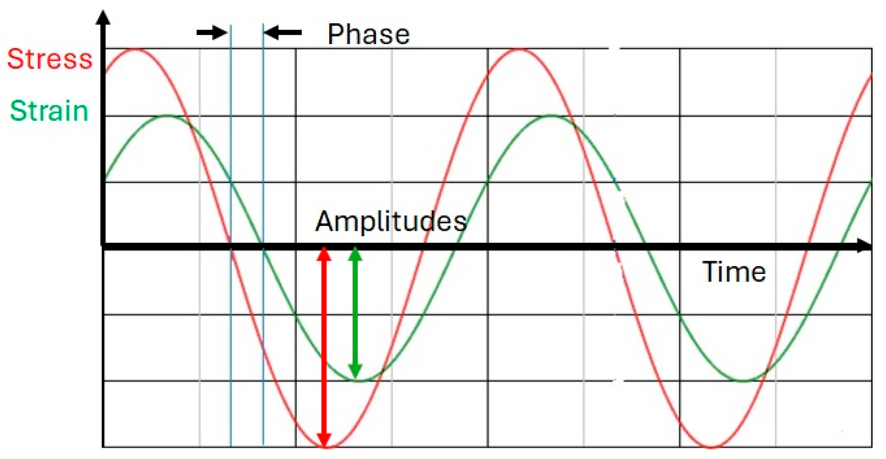
1.3. Elastic and Damping Properties of Composite Materials

The elastic properties of composite material parts are critical in determining their deformation under static and dynamic loads. The vibration and acoustic behavior of these materials are influenced by their elastic and damping properties. Temperature variations change the elastic and damping characteristics of composite materials, leading to alterations in resonance frequencies, mode shapes, and transient responses, which can impact the functional performance of vehicles, construction components, and consumer goods. Therefore, understanding the temperature-dependent elastic and damping properties is essential for a reliable design of composite structures.

The elastic and damping behavior of a material in a thin sheet with linear material properties can be described by engineering constants: Young’s modulus (E), Poisson’s ratio (v), and in-plane shear modulus (G). In a statically loaded sheet, normal stresses and shear stresses occur, resulting in both normal and shear strains. The Young modulus (E) in a material point is the ratio of normal stress to normal strain (see Figure 1a). Poisson’s ratio (v) is the negative ratio of normal strain in one direction to normal strain in the perpendicular direction (see Figure 1b). The in-plane shear modulus (G) is the ratio of shear stress to shear strain (see Figure 1c).

When the sheet is dynamically loaded with a sinusoidal load at a circular frequency (ω), the dynamic Young’s modulus (E(ω)) is the ratio of stress amplitude to strain amplitude (see Figure 2). Similarly, the dynamic Poisson’s ratio (v(ω)) and the dynamic in-plane shear modulus (G(ω)) are the ratios of amplitudes. Damping can cause a phase shift between the sinusoidal stress and strain signals (see Figure 2). This is the case for viscoelastic materials like polymers and polymer composites. The value of the dynamic engineering constants can vary as a function of the circular frequency (see, e.g., Christensen et al. [8]).

For isotropic materials, the elastic properties are the same in each direction. Most composites, however, exhibit orthotropic behavior. Orthotropic materials have elastic properties symmetric with respect to a Cartesian coordinate system. Five engineering constants are required to describe the orthotropic in-plane elastic behavior of thin sheets. In a plane with two perpendicular orthotropic material directions 1 and 2 (see Figure 3), the five engineering constants are E₁ (Young’s modulus in the 1-direction), E₂ (Young’s modulus in the 2-direction), v₁₂ (Major Poisson’s ratio with major strain in the 1-direction and contraction strain in the 2-direction), v₂₁ (Minor Poisson’s ratio with minor strain in the 2-direction and contraction strain in the 1-direction), and G₁₂ (in-plane shear modulus in the (1,2) plane).

The relation between stress and strain in an orthotropic composite sheet is given by the stiffness matrix [C]; see, e.g., Hashin [9]:

$${\mathsf{\sigma }}_{\mathrm{i}}^{\mathrm{*}}={\mathrm{C}}_{\mathrm{i}\mathrm{j}}^{\mathrm{*}}{\mathsf{\epsilon }}_{\mathrm{j}}^{\mathrm{*}} \left(\mathrm{i},\mathrm{j}=1,2,3\right)$$

$$\left\{\begin{array}{c}{\mathsf{\sigma }}_1^{\mathrm{*}}\\ {\mathsf{\sigma }}_2^{\mathrm{*}}\\ {\mathsf{\tau }}_{12}^{\mathrm{*}}\end{array}\right\}=\left[\begin{array}{ccc}{\displaystyle \frac{{\mathrm{E}}_1^{\mathrm{*}}}{1-{\mathsf{\upsilon }}_{12}^{\mathrm{*}}{\mathsf{\upsilon }}_{21}^{\mathrm{*}}}}& {\displaystyle \frac{-{\mathsf{\upsilon }}_{21}^{\mathrm{*}}{\mathrm{E}}_1^{\mathrm{*}}}{1-{\mathsf{\upsilon }}_{12}^{\mathrm{*}}{\mathsf{\upsilon }}_{21}^{\mathrm{*}}}}& 0\\ {\displaystyle \frac{-{\mathsf{\upsilon }}_{12}^{\mathrm{*}}{\mathrm{E}}_2^{\mathrm{*}}}{1-{\mathsf{\upsilon }}_{12}^{\mathrm{*}}{\mathsf{\upsilon }}_{21}^{\mathrm{*}}}}& {\displaystyle \frac{{\mathrm{E}}_2^{\mathrm{*}}}{1-{\mathsf{\upsilon }}_{12}^{\mathrm{*}}{\mathsf{\upsilon }}_{21}^{\mathrm{*}}}}& 0\\ 0& 0& {\mathrm{G}}_{12}^{\mathrm{*}}\end{array}\right]\left\{\begin{array}{c}{\mathsf{\epsilon }}_1^{\mathrm{*}}\\ {\mathsf{\epsilon }}_2^{\mathrm{*}}\\ {\mathsf{\gamma }}_{12}^{\mathrm{*}}\end{array}\right\}$$

(1)

In the case of pure elastic behavior, the engineering constants have only real values. In the case of viscoelastic behavior, the quantities in Equation (1) are all complex numbers with real and imaginary parts. [C*] is the complex in-plane stiffness matrix, ${\epsilon }_1^{\mathrm{*}}$, ${\epsilon }_2^{\mathrm{*}}$ are normal strains, and ${\sigma }_1^{\mathrm{*}}$, ${\sigma }_2^{\mathrm{*}}$ are normal stresses, respectively, in the 1- and 2-direction. ${\gamma }_{12}^{\mathrm{*}}$, ${\tau }_{12}^{\mathrm{*}}$ are the in-plane shear strains and stresses.

$E_1^{\mathrm{*}}$, $E_2^{\mathrm{*}}$ are the complex dynamic Young’s moduli, ${\upsilon }_{12}^{\mathrm{*}}$, ${\upsilon }_{21}^{\mathrm{*}}$ are the major and minor Poisson’s ratios, and $G_{12}^{\mathrm{*}}$ is the complex in-plane shear modulus. For a given circular frequency $\omega$ and assumed linear behavior, the values $E_1^{\mathrm{*}}\hspace{0.33em}{E}_1^{\mathrm{*}}\hspace{0.33em}{\upsilon }_{12}^{\mathrm{*}}\hspace{0.33em}{\upsilon }_{21}^{\mathrm{*}}\hspace{0.33em}{G}_{12}^{\mathrm{*}}$ are constant and called the complex dynamic engineering constants. Because of the symmetry of the stiffness matrix [C*], ${{\upsilon }_{12}^{\mathrm{*}}E}_2^{\mathrm{*}}={{\upsilon }_{21}^{\mathrm{*}}E}_1^{\mathrm{*}}$, and therefore, there are only four independent complex engineering constants in C*. These are shown in Equations (2)–(5).

$$E_1^{\mathrm{*}}=E_1^{\prime }+i.E_1^{″}=E_1^{\prime }\left(1+i.\mathit{tan}\delta \left(E_1\right)\right)$$

(2)

$$E_2^{\mathrm{*}}=E_2^{\prime }+i.E_2^{″}=E_2^{\prime }\left(1+i.\mathit{tan}\delta \left(E_2\right)\right)$$

(3)

$$v_{12}^{\mathrm{*}}=v_{12}^{\prime }+i.v_{12}^{″}=v_{12}^{\prime }(1+i.\mathit{tan}\delta ({\upsilon }_{12}\left)\right)$$

(4)

$$G_{12}^{\mathrm{*}}=G_{12}^{\prime }+i.G_{12}^{″}=G_{12}^{\prime }(1+i.\mathit{tan}\delta (G_{12}\left)\right)$$

(5)

The real parts in Equations (2)–(5) represent the elastic behavior, while the imaginary “tangents delta” parts govern the damping contribution in the complex engineering constants.

1.4. A Novel Setup to Measure Orthotropic Engineering Constants

A novel measurement setup utilizing a non-destructive impulse excitation method has been developed for the automated identification of complex orthotropic engineering constants as a function of temperature. In this study, the measurement setup is employed to provide a comparative analysis of the identified engineering constants of glass and basalt bidirectionally fabric-reinforced composites with an epoxy matrix, across a temperature range from −20 °C to 60 °C. The first chapter of this article will describe briefly static standard methods, standard dynamic methods, and the new measurement setup. Subsequently, the tested materials and measurement results will be discussed.

2. Measurement of Engineering Constants of Composite Materials

Various test methods exist for measuring engineering constants, categorized into static and dynamic measurement methods.

2.1. Static Measurement Methods

Well-known static methods include tensile testing, bending, shear, and torsion tests. Engineering constants are determined based on measured forces and longitudinal and transverse deformations (see, e.g., ASTM D3039 [10]). Flexural testing in three- or four-point bending is an alternative to tensile testing, applying much smaller forces and achieving larger displacements. Calculations are typically based on thin-beam flexure equations, as described in ASTM D7264/D7264M-21 [11]. Experimental results always come with a level of uncertainty. Factors affecting uncertainty in static testing are discussed by Kostic et al. [12]. The most influential source of uncertainty in determining the engineering constants of composite materials via static testing is the test system (dimensional measurement device, gauge determination system, extensometer type, alignment system, test machine stiffness, force measurement accuracy, and extensometer accuracy), as noted by Lord and Morrell [13]. Due to inevitable imperfections in the sensors, force and displacement measurements at low stress and strain values near the origin of the stress–strain curve have high relative uncertainty bounds.

2.2. Dynamic Measurement Methods

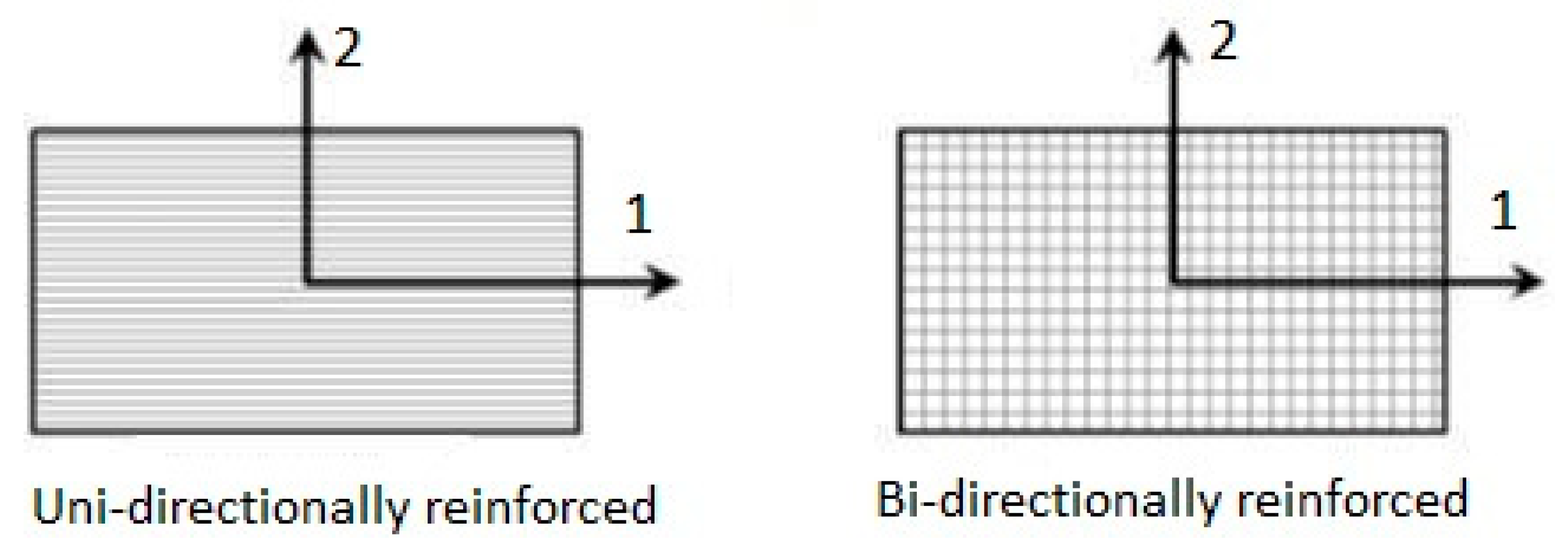
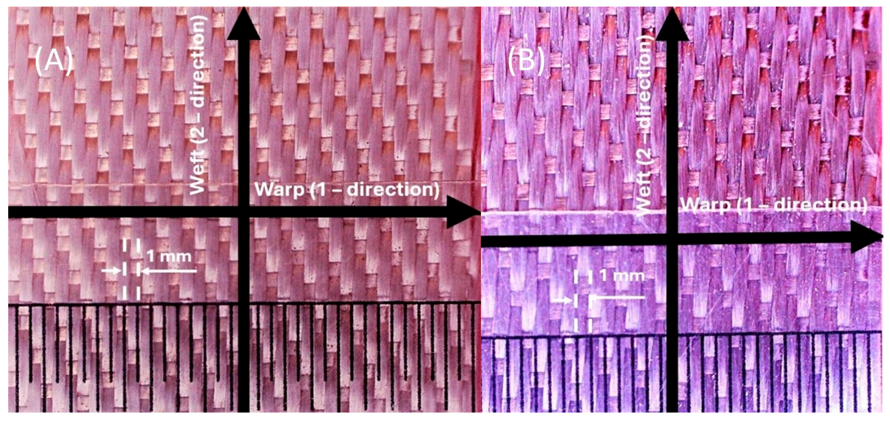
Dynamic testing methods are indirect. The impulse excitation technique (IET) (see, e.g., ASTM C1259 [14]) and dynamic mechanical analysis (DMA) (see, e.g., the work of Schalnat et al. [15]) are the most used dynamic methods. Dynamic testing methods are more challenging to understand intuitively but are easier to execute and provide more accurate engineering constants at low stress and strain amplitudes, as noted by Lord and Morrell [13]. The DMA uses forced excitation to measure the elastic and damping properties of composite beams within a limited frequency range, allowing the identification of temperature and frequency-dependent elastic and damping properties. Unfortunately, most DMA equipment can only handle small beam samples, which is a disadvantage for testing composite materials, as discussed by Ashok et al. [16]. IET can be easily applied to large beam samples, is easy to perform, and does not require complex equipment. Simply tapping the test sample causes a low-amplitude vibration response that can be measured with a sensor and is called the “impulse response function” (IRF). The IRF comprises decaying excited modes of vibration of the test sample. The resonance frequencies and damping ratios can be extracted from the measured IRF, Heritage et al. [17]. Because IET is non-destructive, it is suitable for testing at different temperatures, as per Brebels et al. [18]. Because of all these advantages, IET was selected for the current study. The standard IET uses analytical and empirical formulas to derive the elastic properties from the measured vibration quantities. Unfortunately, no formulas are available for freely suspended orthotropic plates. To solve this problem, Sol [19] demonstrated in 1986 the possibility of replacing standard IET formulas with special-purpose finite-element (FE) models. He used a mixed numerical-experimental technique (MNET) to identify orthotropic engineering constants. The resulting identification method, called the ‘Resonalyser’ procedure, can simultaneously identify the four engineering constants of an orthotropic material from resonance frequencies of two test beams and a test plate measured by IET. The Resonalyser procedure is a multi-sample IET that extracts the resonance frequencies and damping ratios from the measured IRFs on a thin orthotropic rectangular test plate and two test beams. The test beams were cut along two in-plane orthotropic directions (Figure 4). The length-to-width ratio L/W of the test plate was adjusted according to the following Equation (6):

$${\displaystyle \frac{L}{W}}=\sqrt[2]{{\displaystyle \frac{f_1{L}_2}{f_2{L}_1}}}$$

(6)

The resonance frequencies f₁ and f₂ were associated with the fundamental bending vibration modes of the two test beams. L₁ and L₂ are the lengths of the beams. The aspect ratio L/W creates the so-called “Poisson” plate. The physical background of Equation (6) is an imaginary plate with a zero Poisson’s ratio. Hence, the plate acts as a beam in both the 1- and 2-direction. The aspect ratio L/W makes the resonance frequencies of both beam vibrations equal. Equation (6) is valid for any orthotropic material. The first five resonance frequencies of a Poisson plate are always associated with torsion, saddle, breathing, and two combinations of torsion and bending vibration modes (see Figure 5).

The modal shapes shown in Figure 5 were computed with the Resonalyser software v1.0 for a Poisson plate. The orthotropic engineering constants are parameters in the numerical models of the beams and plate. These were iteratively tuned to match the computed resonance frequencies with the measured frequencies. Because the vibration modes of the first five resonance frequencies are known, no full modal analysis is necessary to identify the type of vibration mode sequence. An interesting property of a Poisson plate is that the saddle and breathing vibration modes are highly sensitive to variations in Poisson’s ratio, as shown by Lauwagie et al. [20]. Knowledge of the type of vibration mode, together with the first three measured resonance frequencies, allows the generation of good starting values for the engineering constants G₁₂ and v₁₂ using the virtual field method, as per Pierron et al. [21]. A detailed mathematical derivation can be found in a study by Sol et al. [22]. Validation of the results obtained using the Resonalyser procedure has been presented in several publications [23,24,25]. In 1995, De Visscher et al. [26] extended the Resonalyser procedure to identify the damping part of the complex orthotropic engineering constants. Detailed information on how the damping part can be computed from the measured FRF can be found in [26]. Information and examples of the extended Resonalyser method can be found in Bytec [27].

Over the past few decades, various authors have presented MNET approaches for identifying orthotropic elastic constants [28,29,30,31,32,33,34,35,36,37,38,39,40,41,42,43,44]. Most methods require the measurement of modal shapes associated with resonance frequencies by using experimental modal analysis techniques. Modal analysis allows for measurement on large composite material plate samples, but it is more difficult to execute as a function of temperature than IET. Therefore, the extended Resonalyser procedure was selected for the continuous identification of engineering constants across different temperatures in a climate chamber. At different temperature steps across a desired temperature range, the IRF of the test beams and the Poisson plate were obtained using an automated excitation system. This allowed for the identification of the orthotropic engineering constants at each temperature step. Automated excitation uses a pendulum impact activated by solenoids. The pendulum was connected through a small aperture in the climate chamber wall (Figure 6).

The pendulum mechanism is actuated using a solenoid (yellow in Figure 6a). Upon activation via voltage, the solenoid propels a lever (dark blue in Figure 6), which strikes the wall of the climate chamber. Owing to inertia, the pendulum was set in motion until it impacted the sample (red star in Figure 6b). The sample received an impulse and oscillated, while the pendulum mass rebounded. Gravity pulls the lever back to its initial position (Figure 6c). All components of the pendulum mechanism returned to their starting positions, while the sample continued to oscillate (Figure 6c). Three pendulum systems simultaneously excited the two beams and the plate sample in the climate chamber.

It is essential that the temperature distribution within the sample remains homogeneous across all temperature steps. The transient heat conduction in a thin sheet is influenced by convection occurring at the surfaces. The temperature profile of the samples varies over time at different internal positions, with the surface temperature changing relatively quickly, whereas the temperature at the midplane changes more slowly. Key control parameters include the convection heat-transfer coefficient h, thermal conductivity k, specific heat capacity Cp, and density ρ of the composite material of the sample, as discussed in the book of Cengel [45]. The delay time between subsequent temperature steps was tested previously in the laboratory for different materials using embedded thermocouples. For thin composite material plates (thickness smaller than 10 mm) and good homogeneous quality test materials, the measured temperature evolved according to the theory. The modified epoxy matrix of the GFRC and BFRC has relatively good conductivity properties, and the samples in this study are relatively thin (2–3 mm). The delay time for the measurements in this study was taken as 5 min for each step of 1 °C. This yields a variation of less than 0.1 °C in the middle of the samples as compared to the surface temperature. However, due to the weaving and laminated structure of the samples, 100% homogeneity of temperature at every point is not possible. Further details on the automated excitation and temperature distribution in the test samples can be found in the work of Sol et al. [28].

A description of the tested materials and a graphical representation of the test results are provided in the next chapter. At the end of this paper, a comparison of the elastic and damping behavior between GFRP and BFRP in a temperature range of −20 °C to 60 °C is provided.

3. Tested Materials

The aim of this study was to compare two similar samples, the major difference being the type of fiber reinforcement. The first sample, a bidirectional glass G300 fabric reinforced composite sample GFRP had an MTB350-enhanced epoxy matrix and was composed of eight layers with a weave pattern known as “8-Harness Satin” (8HS). The fiber volume fraction was 47%. The sample thickness was 2 mm, and the density was 1874 kg/m³. Figure 7A shows a patch of this 8HS glass fabric.

The second sample, a bidirectional basalt TT320 fabric-reinforced composite sample BFRP, had an MTB350-enhanced epoxy matrix and was composed of eight layers with a 7HS weave pattern. The fiber volume fraction was 45%. The sample thickness was 2.17 mm, and the density was 1876 kg/m³. Figure 7B shows a patch of basalt 7HS fabric. Both the basalt and the glass fibers were treated with the same silane coupling agent. The warp direction for both samples in Figure 7 is referred to as the 1-direction or 0° direction. The weft direction is referred to as the 2-direction or 90° direction. The interfacial shear strength of the BFRC and GFRC samples was measured by the SHD composite laboratory (Sleaford, UK): 63.0 MPa and 69.8 MPa for, respectively, the warp direction of the glass and basalt sample, and 58.7 MPa and 58.4 MPa for, respectively, the weft direction of the glass and basalt sample.

A 7HS weave pattern is only slightly stiffer in the weft direction than an 8HS weave pattern. The sizes and masses of the tested beams and plates are presented in

Table 1. Dimensions and masses of the test beams and plates.

Sample	Length [mm]	Width [mm]	Thickness [mm]	Mass [g]
GFRP Beam-1 (0°)	255	25.9	2.00	24.9
GFRP Beam-2 (90°)	272	26.0	2.03	26.8
GFRP plate	243	234	2.03	217.0
BFRP Beam-1 (0°)	247	26.0	2.17	26.2
BFRP Beam-2 (90°)	273	26.0	2.17	28.9
BFRP plate	243	239	2.23	243.0

All the samples were preconditioned in the climate chamber at 20 °C and a relative humidity of 50%.

.

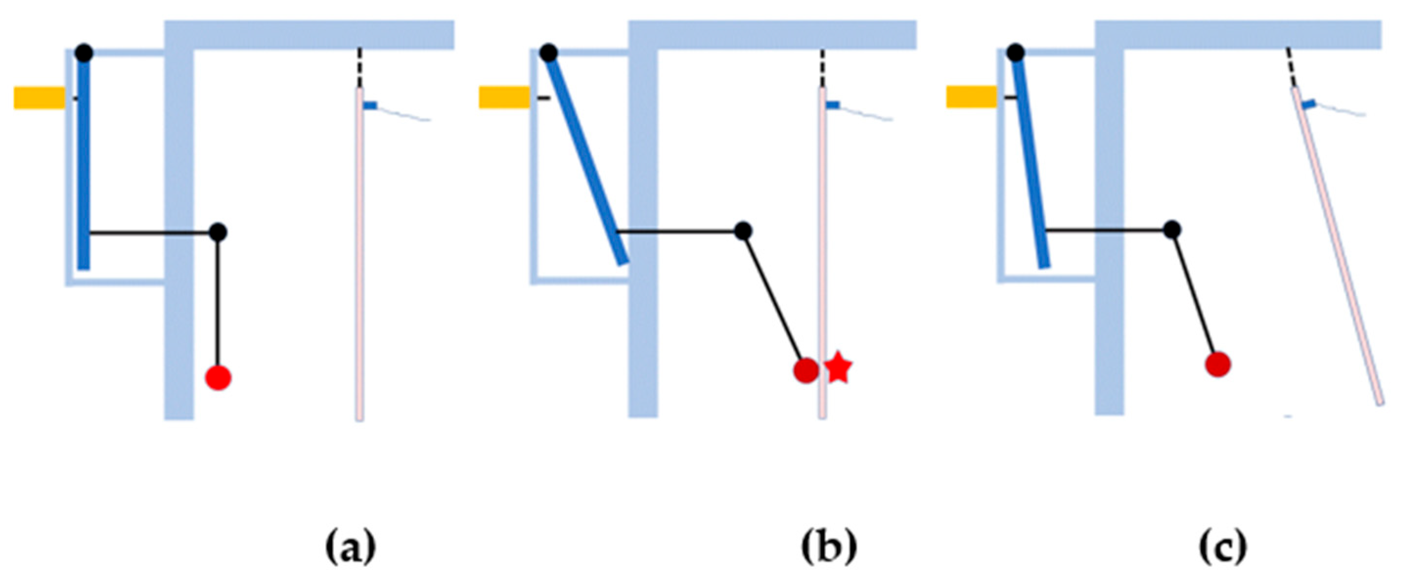
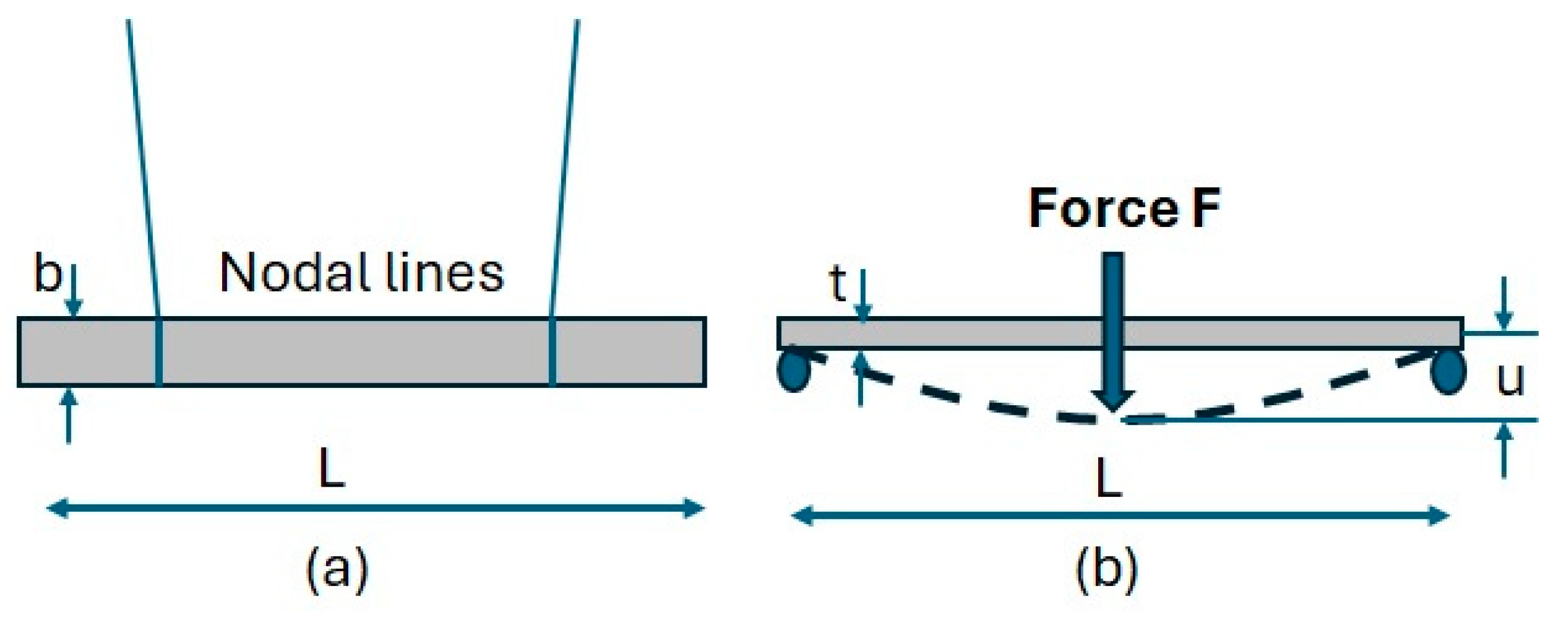
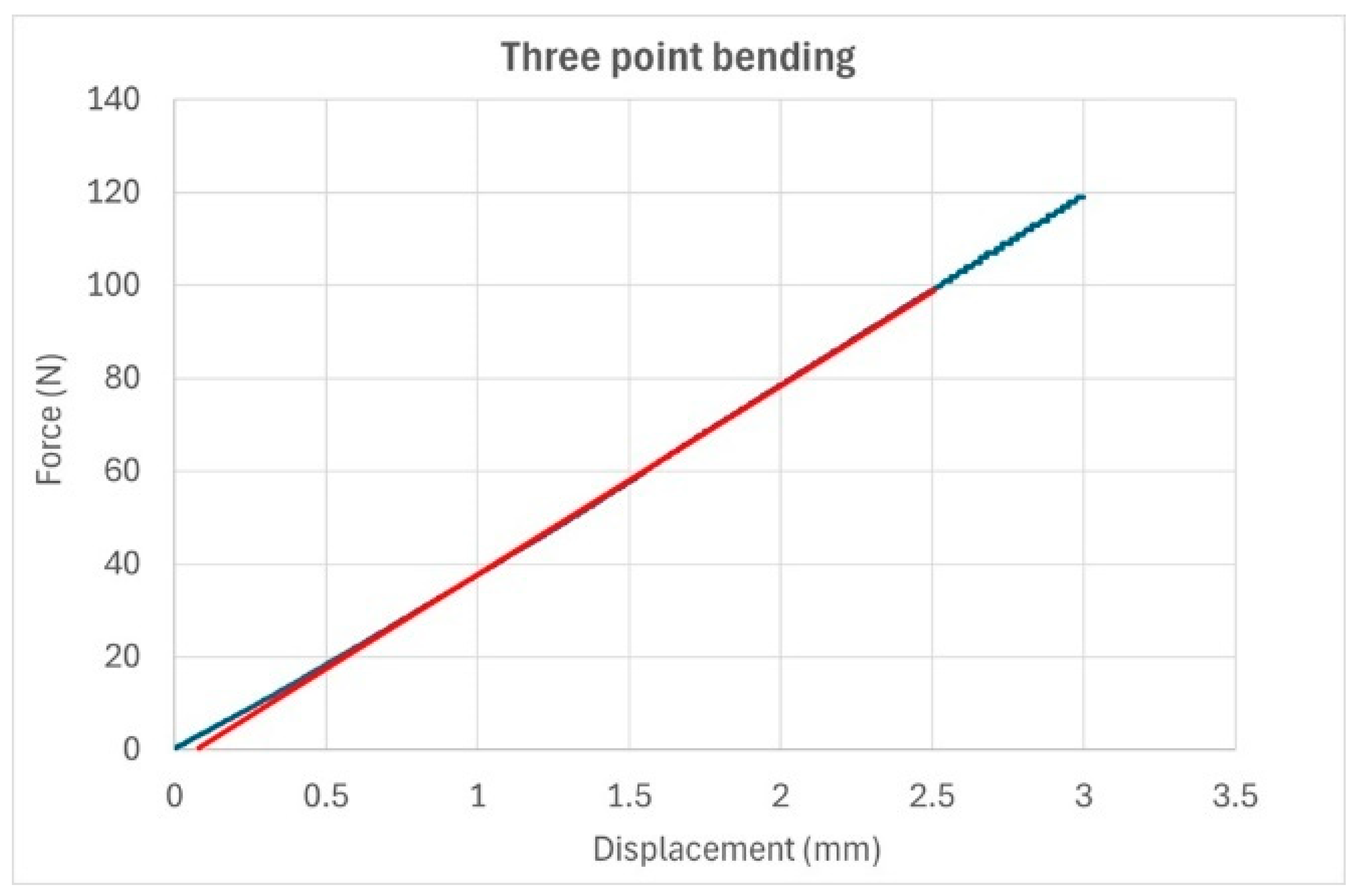
4. Measurement of Young’s Modulus by Three-Point Bending and IET

The standard EIT was executed continuously across a temperature range of −20 °C to 60 °C on the same test samples in an ARS 0390 climate chamber manufactured by ESPEC CORP. Contrary to static testing, IET directly provides Young’s modulus at very low displacement and force values using the formula provided in ASTM C 1259–98 [14]:

$$E=0.972{\displaystyle \frac{f^2{L}^{3}M}{b{t}^3}}$$

(7)

As a result of an impact with a small hammer, the test sample vibrates mainly on its fundamental bending modal shape. Nodal lines are positions where the vibration amplitude is zero. The sample is freely suspended with thin wires, fixed on the nodal line position to minimize the influence of the wires on the IRF. A microphone is used as a sensor to measure the IRF. In Equation (7), f is the frequency measured on a test beam freely suspended in its nodal lines (Figure 8), L is the length of the beam, M is the mass, b is the width, and t is the thickness.

Experimental results always come with a level of uncertainty. The uncertainty estimation of Young’s modulus E, as found by Equation (7), can be computed by evaluating all the uncertainties of the contributing parameters in the formula. The uncertainty expressed as a relative percentage on the measured frequency f is 0.1%, the uncertainty on the measured mass M is 0.01%, the uncertainty of the length L is 0.4%, the uncertainty on the width is 0.04%, and the uncertainty on the thickness t is 0.3%. The computed relative percentage on the Young’s modulus with (7) is, hence, 1.8%.

The three-point bending test was conducted using a universal testing machine, Tinius Olsen 5 ST, across a temperature range of −20 °C to 60 °C, with increments of 10 °C. The test bench was housed in a temperature chamber (TH2700) manufactured by Grip Engineering GmbH, Nurenberg, Germany. The cooling was facilitated by liquid nitrogen, which was controlled by a magnet valve located at the back of the chamber. The instrument was equipped with a 2.5 kN load cell, and measurements were taken with a span of 80 mm and a displacement speed of 1 mm/min. The accuracy of the load cell and displacement was 1%. The Young’s modulus of the three-point bending test could not be computed directly from the force and displacement near the origin because of the uncertainty of the force and displacement values at very low values. Therefore, the Young’s modulus of the samples was calculated using linear regression between a force of 100 Newtons and zero. Figure 9 shows an example of a recorded force–displacement curve. The red line in Figure 9 is the regression line.

The measurement procedure and formula for the computation of Young’s modulus are given in ASTM D7264/D7264M-21 [11] (see Figure 8b also):

$$E={\displaystyle \frac{F{L}^3}{4ub{t}^3}}$$

(8)

In Equation (8), F = 100 Newton is applied in the middle of the span, L = 80 mm is the length of the span between the supports, u is the displacement measured by curve fitting between zero and 100 Newton, b is the width, and t is the thickness. Since the measurement of a force F and a deflection u in three-point bending is less accurate, the uncertainty estimation on E according to Equation (8) yields a higher value, namely 3%.

In

Table 2. Test results for the Young’s modulus (E1 and E2) of GFRP.

	Young’s Modulus E1 (0°) [GPa]				Young’s Modulus E2 (90°) [GPa]
Temperature [°C]	3-pb *	Δ **	IET	Δ **	3-pb *	Δ **	IET	Δ **
−20	26.6	0.8	27.8	0.5	23.6	0.7	25.7	0.5
−10	26.3	0.8	27.6	0.5	24.2	0.7	25.5	0.5
0	26.0	0.8	27.4	0.5	24.0	0.7	25.4	0.5
10	26.8	0.8	27.2	0.5	24.0	0.7	25.2	0.5
20	25.5	0.7	27.1	0.5	23.7	0.7	25.0	0.5
30	25.6	0.7	26.9	0.4	23.4	0.7	24.8	0.5
40	24.7	0.7	26.7	0.4	22.5	0.6	24.6	0.5
50	24.3	0.7	26.5	0.4	21.9	0.6	24.4	0.5
60	24.0	0.7	26.2	0.4	21.6	0.6	24.0	0.5

* Three-point bending. ** Uncertainty estimation.

and

Table 3. Test results for the Young’s modulus (E₁ and E₂) of BFRP.

	Young’s Modulus E1 (0°) [GPa]				Young’s Modulus E2 (90°) [GPa]
Temperature [°C]	3-pb *	Δ **	IET	Δ **	3-pb *	Δ **	IET	Δ **
−20	25.1	0.7	26.1	0.5	23.3	0.7	25.8	0.5
−10	23.6	0.7	26.0	0.5	23.6	0.7	25.6	0.5
0	24.0	0.7	25.8	0.5	24.3	0.7	25.5	0.5
10	23.9	0.7	25.6	0.5	23.2	0.7	25.3	0.5
20	23.9	0.7	25.4	0.5	22.9	0.7	25.1	0.5
30	24.2	0.7	25.3	0.5	22.4	0.7	24.8	0.5
40	22.6	0.7	25.0	0.5	22.2	0.6	24.7	0.5
50	22.2	0.6	24.8	0.4	21.9	0.6	24.5	0.5
60	21.9	0.6	24.4	0.4	21.4	0.6	24.0	0.5

* Three-point bending. ** Uncertainty estimation.

, “3-pb” stands for three-point bending, “Δ” denotes the estimated uncertainty, and “IET” denotes the impulse excitation technique results.

In Figure 10, it can be observed that the difference between the Young’s moduli E₁ and E₂ of GFRP and BFRP was very small. It can also be seen that the static three-point bending results are systematically slightly lower than the values from the dynamic IET tests. This can be explained by the viscoelastic nature of fiber-reinforced polymers (see, e.g., Christensen et al. [8]).

5. Automated Testing with the Extended Resonalyser Procedure

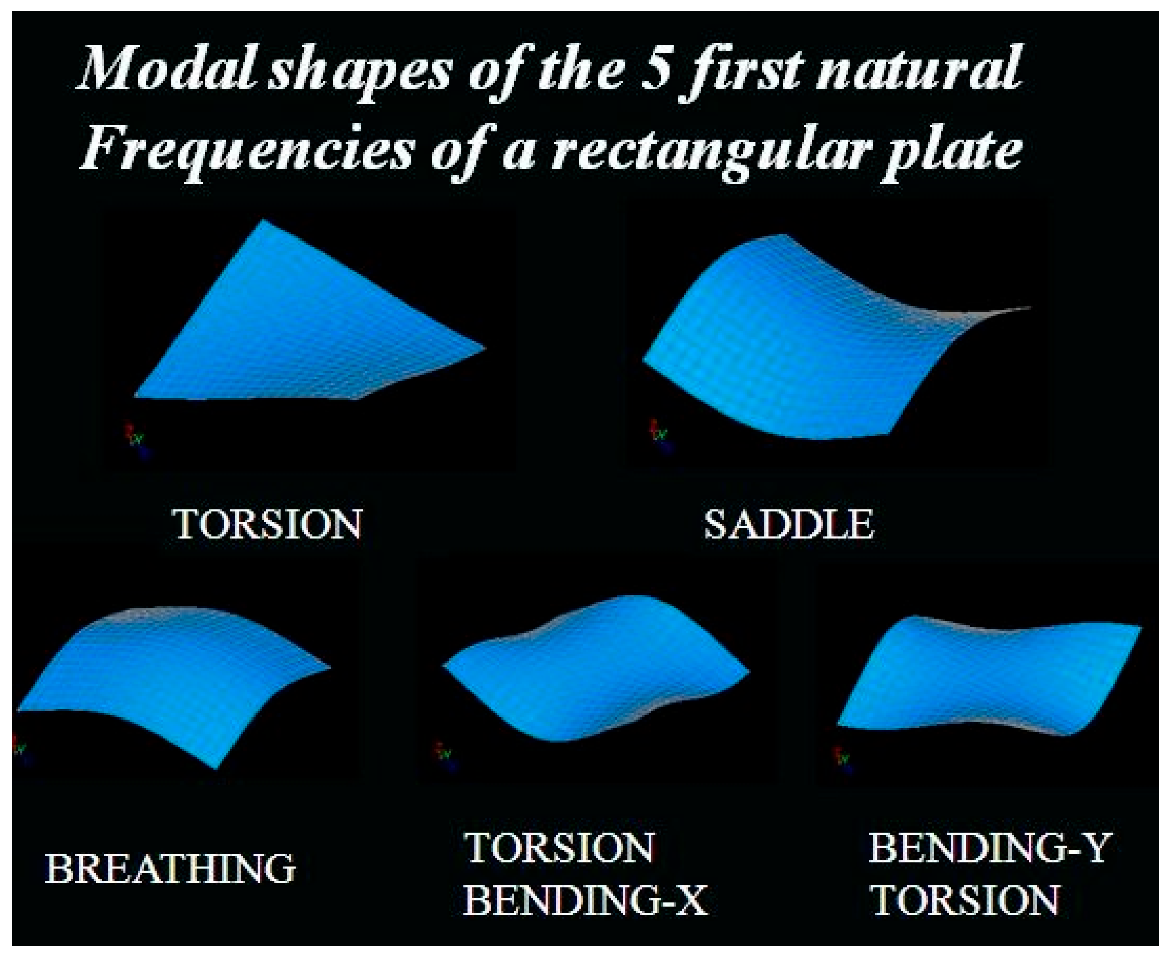
5.1. Measurement Results (Frequency and Damping Ratio Plots)

The Resonalyser is a multi-sample mixed numerical experimental technique based on the measurement of the first resonance frequencies and damping ratios associated with the fundamental flexural modal shape of two beams, two resonance frequencies, and the damping ratios of the test plate associated with the torsion and breathing modal shapes.

Figure 11 and Figure 12 show the results obtained by using automated IET testing equipment. The resonance frequencies associated with the fundamental bending modal shapes of Beam 1 (Figure 11a) and Beam 2 (Figure 11b), the resonance frequency associated with the torsional modal shape (Figure 11c), and the resonance frequencies associated with the breathing modal shape (Figure 11d) of both the GFRP and BFRP samples are shown in Figure 11. The resonance frequencies of the basalt-reinforced samples (brown in Figure 11) are slightly higher than those of the glass-reinforced samples (blue in Figure 11). All measured frequencies decreased monotonously with increasing temperature. Figure 12 shows the measured damping ratios of the test beams and the Poisson plate. It can be observed in Figure 12 that the damping curves (thin blue and brown lines) show more noise than the measured frequencies in Figure 11. The damping curves were, therefore, smoothed with polynomials (thick blue and brown lines) before their values were used for identification of the damping part of the engineering constants (see Figure 12).

The damping ratios associated with the fundamental bending modal shapes of Beam 1 (Figure 12a) and Beam 2 (Figure 12b), the damping ratio associated with the torsional modal shape (Figure 12c), and the damping ratios associated with the breathing modal shape (Figure 12d) of both the GFRP and BFRP samples are shown in Figure 12.

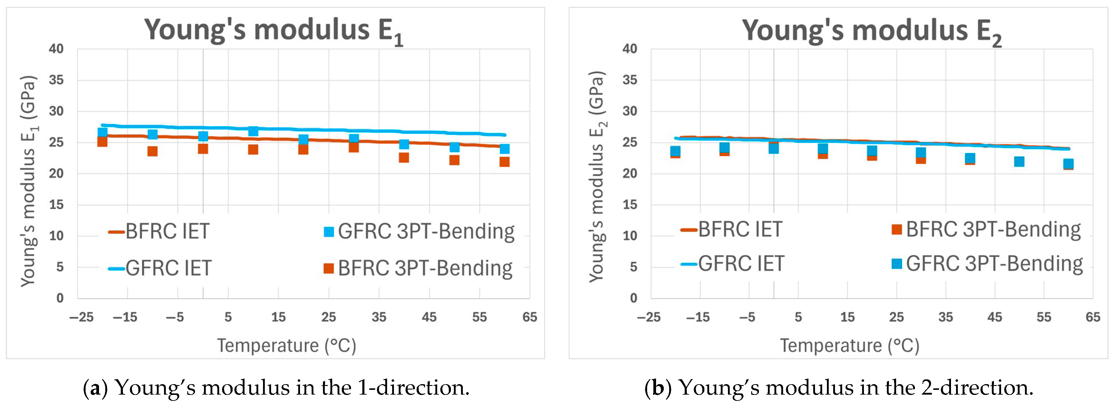
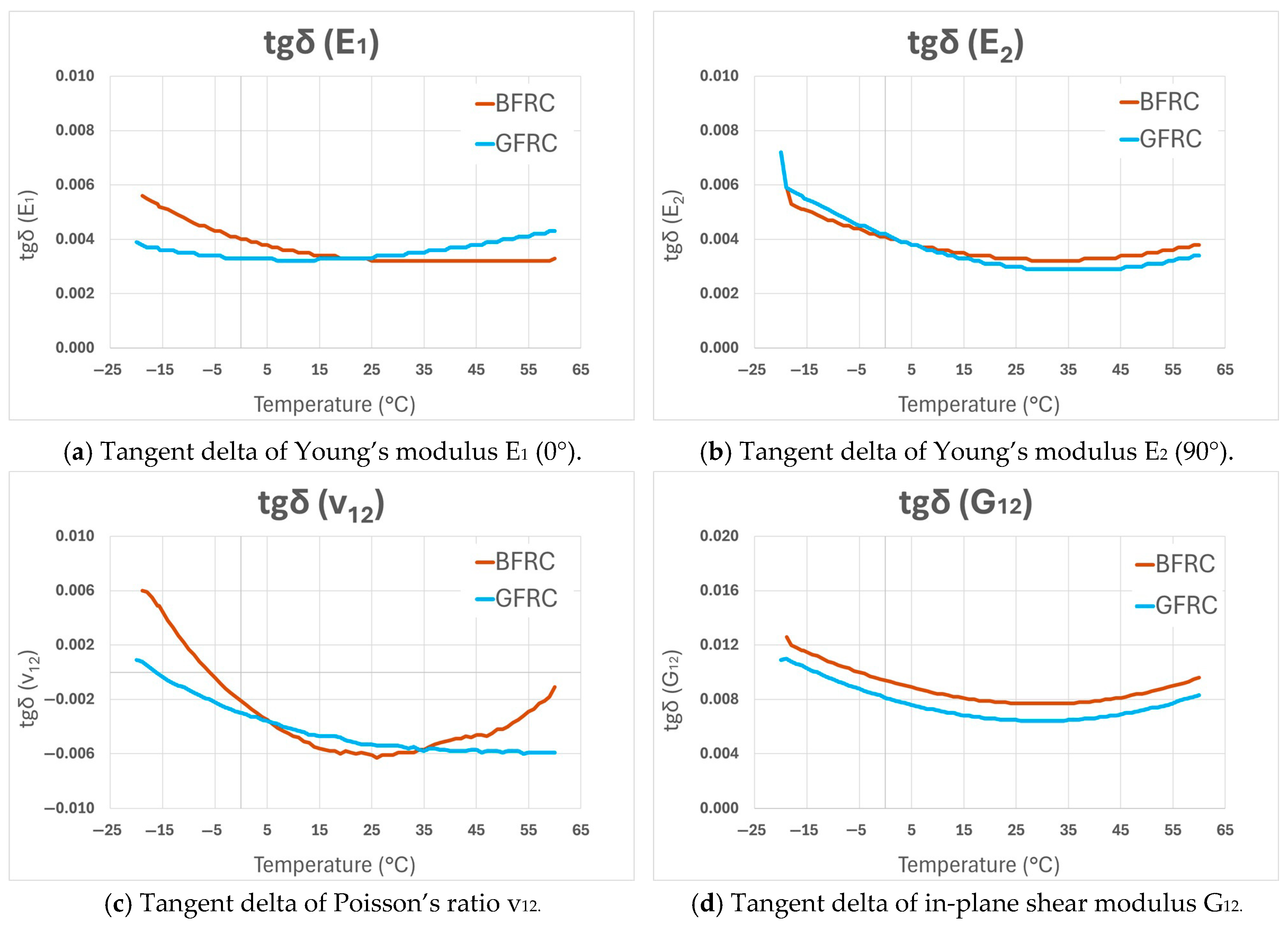
5.2. Identified Engineering Constants (Moduli and Tangents Delta)

In the Resonalyser procedure, the complex engineering constants in the numerical models of the two test beams and the test plate are iteratively updated till the computed resonance frequencies and damping ratios match the measured values.

At each temperature step, the measured resonance frequencies and damping ratios were used in the Resonalyser procedure to identify the real (elastic) part and tangent delta (damping) part of the orthotropic engineering constants of the GFRP and BFRP samples between −20 °C and 60 °C. The results are shown in Figure 13 (real part) and Figure 14 (tangent delta). It can be observed in Figure 13a that the values of Young’s modulus E₁ in the warp direction of GFRP are slightly larger than those of BFRP for the whole considered temperature range. The values of the Young’s moduli in the weft direction E₂ of GFRP (Figure 13b) are equal to those of BFRP for all temperatures: both curves coincide.

The same observation of coincidence is valid for both curves of Poisson’s ratio in Figure 13c. The shear modulus curves have the same evolution as the Young’s modulus in the warp direction; the G₁₂ values of the GFRP curve are slightly larger than those of BFRP for the whole considered temperature range. Finally, it can be remarked that all the curves of Figure 13 have decreasing values from −20 °C towards 60 °C. It can be observed in Figure 13a that the Young’s modulus E₁ (warp direction) of GFRC is slightly stiffer than the Young’s modulus E₁ of BFRC. The same observation is true for the shear modulus G₁₂. However, Figure 13b shows that the Young’s modulus E₂ (weft direction) for both materials seems to be equal. This can be explained by the fact that the 7HS weave in the BFRC is slightly stiffer than the 8HS weave in GFRC.

The same BFRC and GFRC were tested statistically by the SHD Laboratory (Sleaford, UK), with tensile and flexural testing at room temperature conditions (J543) in agreement with ISO norms.

Table 4. Engineering constants of GFRC measured by the SHD Laboratory.

Engineering Constant	Tensile Test [46]		Flexural Test [47]
	Value	StDev	Value	StDev
Young’s modulus E1 (0°)	23.9 GPa	0.1	25.2 GPa	0.4
Young’s modulus E2 (90°)	22.6 GPa	0.3	23.9 GPa	0.4
Poisson’s ratio V12	0.18	-	0.18	-

shows the results for E₁, E₂, and v₁₂ for GFRC.

Table 5. Engineering constants of BFRC measured by the SHD Laboratory.

Engineering Constant	Tensile Test [46]		Flexural Test [47]
	Value	StDev	Value	StDev
Young’s modulus E1 (0°)	24.2 GPa	0.3	22.4 GPa	0.4
Young’s modulus E2 (90°)	23.2 GPa	0.3	22.6 GPa	0.4
Poisson’s ratio V12	0.18	-	0.17	-

shows similar results for BFRC.

The values in Table 4 and Table 5 are slightly lower than the Resonalyser values presented in Figure 13. This is like the observations in Figure 10 and reveals, again, the viscoelastic nature of the BFRC and GFRC.

The curves for the tangent delta in Figure 14 are nearly coinciding but are not monotonously decreasing like the real parts of the engineering constants. The curves show minimal values around room temperature and then increase slowly with increasing temperature. The glass transition onset temperature for the used MTB350 modified epoxy resin matrix after 1 h curing was measured by the SDH laboratory (Sleaford, UK) and was equal to 144 °C, which is much higher than the maximum temperature of 60 °C in the current study.

6. Discussion

The temperature interval from −20 °C to 60 °C was selected for its relevance to many vehicles and consumer goods. Generally, the observation is that the differences of the engineering constants between the GFRP and BFRP are minimal in this studied temperature interval. Some details, however, require some discussion. In Figure 11, all the frequency values of the BFRP beam samples are larger than those of the GFRP, while in Figure 13, the Young’s moduli of the GFRP beams appear to be larger than those of the BFRP beams. This can be explained by the larger thickness value of the BFRP beams (about 2.2 mm) as compared to the thickness of the GFRP beams (about 2 mm). The resonance frequencies of beams increase linearly with thickness t, as can be seen by rewriting Equation (8) into Equation (10), taking Equation (9) into account:

$$M=\rho Lbt$$

(9)

$$f={\displaystyle \frac{1.028}{L^2}}.t.\sqrt{{\displaystyle \frac{E}{\rho }}}$$

(10)

Table 6. Young’s moduli E₁ and E₂ of GFRC and BFRC.

Young’s Moduli	Resonalyser MPa	Three-Point Bending MPa	Flexural Test SDH MPa	Tensile Test SDH MPa
GFRC E1 (0°)	27.1	25.5	23.9	25.2
GFRC E2 (90°)	25.0	23.7	22.6	23.9
BFRC E1 (0°)	25.4	23.9	24.2	22.4
BFRC E2 (90°)	25.1	22.9	23.2	22.6

summarizes the results for the Young’s moduli E₁ and E₂ for the GFRC and GFRC samples at room temperature (20 °C).

A first observation from Table 6 is that the dynamic Resonalyser values are slightly larger than the static tensile and flexural values, which reveals the visco-elastic nature of the GFRC and BFRC samples. A second observation is that the Young’s modulus E1 in the warp (0°) of the GFRC is slightly higher than the modulus of the BFRC. The Young’s modulus E₂ in the weft (90°) direction of the GFRC nearly equals the value of the BFRC. This can be explained by the fact that the 7HS weave in the BFRC is slightly stiffer than the 8HS weave in the GFRC.

The measured damping ratios as a function of temperature in the plots of Figure 12 show more noise than the plots of the measured frequencies in Figure 11. The explanation for this observation is that damping is principally governed by the matrix of the composites. The temperature distribution in the matrix at subsequent temperature steps can never be 100% homogeneous in all positions in the samples. The temperature heterogeneities cause variations in the damping value. The measured frequencies are principally governed by the stiffness of the fiber reinforcements, which are less influenced by small temperature fluctuations.

The increase in the delta tangent values towards 60 °C is very small. This is an indication that 60 °C is still far from the glass transition onset temperature of the matrix material at 144 °C. The resonance frequencies during the Resonalyser measurements vary in an interval starting from 70 Hz (Torsion) to 160 Hz (Breathing). The behavior of GFRC and BFRC for higher frequencies is not considered in this study. The visco-elastic nature of the samples is revealed by the lower values of the engineering constants for the static tests. As for all the experimental results, caution should be taken when using the results of simulations of composite material parts in other conditions than the test conditions described in this study, e.g., changes in the values of engineering constants by pre-loads, as discussed, e.g., by Ayorinde [41], higher frequencies ranges for acoustical applications, and other environmental conditions).

7. Conclusions

The IET was selected for the described study because of its many advantages as a dynamic method. It is non-destructive, accurate, and easy to automate. The proposed automated Resonalyser procedure simultaneously uses IET on two beams and a Poisson plate and allows for the identification of complex orthotropic engineering constants as a function of temperature. The results were validated as much as possible by tensile and flexural tests. No experimental modal analysis is required for the described automated Resonalyser procedure. The resulting engineering constants are identified at low strains and stresses and, hence, are suitable for usage in the linear analysis of deformations of construction parts. Engineering constants are mechanical parameters that are necessary for linear deformation analysis and vibration studies. In the presented study, no major differences between the engineering constants of glass- and basalt-reinforced composites in the considered temperature interval of −20 °C to 60 °C could be found. For applications in which the strength of the materials is important, only a study with appropriate static methods in the same temperature range can provide answers.

References

1. Sathishkumar, T.P.; Satheeshkumar, S.; Naveen, J. Glass fiber-reinforced polymer composites—A review. J. Reinf. Plast. Compos. 2014, 33, 1258–1275. [Google Scholar] [CrossRef]
2. Singh, J.; Kumar, M.; Kumar, S.; Mohapatra, S.K. Properties of Glass Fiber Hybrid Composites: A Review. Polym.-Plast. Technol. Eng. 2017, 56, 455–469. [Google Scholar] [CrossRef]
3. Pirzada, M.M. Recent Trends and Modifications in Glass Fibre Composites—A Review. Int. J. Mater. Chem. 2015, 5, 117–122. [Google Scholar]
4. Jamshaid, H.; Mishra, R. A green material from rock: Basalt fiber—A review. J. Text. Inst. 2016, 107, 923–937. [Google Scholar] [CrossRef]
5. Sbahieh, S.; Mckay, G.; Al-Ghamdi, S.G. A comparative life cycle assessment of fiber-reinforced polymers as a sustainable reinforcement option in concrete beams. Front. Built Environ. 2023, 9, 1194121. [Google Scholar] [CrossRef]
6. Lapena, M.H.; Marinucci, G. Mechanical Characterization of Basalt and Glass Fiber Epoxy Composite Tube. Mater. Res. 2018, 21, e20170324. [Google Scholar] [CrossRef]
7. Tavadi, A.R.; Naik, Y.; Kumaresan, K.; Jamadar, N.I.; Rajaravi, C. Basalt fiber and its composite manufacturing and applications: An overview. Int. J. Eng. Sci. Technol. 2021, 13, 50–56. [Google Scholar] [CrossRef]
8. Christensen, R.M. Theory of Viscoelasticity an Introduction; Academic Press: Cambridge, MA, USA, 1971. [Google Scholar]
9. Hashin, Z.V.I. Complex moduli of viscoelastic composites: General theory and application to particulate composites. Int. J. Solids Struct. 1970, 6, 539–552. [Google Scholar] [CrossRef]
10. ASTM D3039; Standard Test Method for Tensile Properties of Polymer Matrix Composite Materials. ASTM: West Conshohocken, PA, USA, 2017; ASTM D3039/D3039M-17 from ASTM.org.
11. ASTMD7264/D7264M-21; Standard Test Method for Flexural Properties of Polymer Matrix Composite Materials. ASTM: West Conshohocken, PA, USA, 2021. [CrossRef]
12. Kostic, S.; Miljojkovic, J.; Simunovic, G.; Vukelic, D.; Tadic, B. Uncertainty in the determination of elastic modulus by tensile testing. Eng. Sci. Technol. Int. J. 2022, 25, 100998. [Google Scholar] [CrossRef]
13. Lord, J.D.; Morrell, R.M. Elastic Modulus Measurement, Good Practice Guide No. 98; Elastic Modulus Measurement|NPL Publications; National Physical Laboratory: London, UK, 2006. [Google Scholar]
14. ASTMC 1259–98; Standard Test Methods for Dynamic Young’s Modulus, Shear Modulus and Poisson’s Ratio for Advanced Ceramics by Impulse Excitation of Vibration. ASTM: West Conshohocken, PA, USA, 2022. [CrossRef]
15. Schalnat, J.; Gómez, D.G.; Daelemans, L.; De Baere, I.; De Clerck, K.; Van Paepegem, W. Influencing parameters on measurement accuracy in dynamic mechanical analysis of thermoplastic polymers and their composites. Polym. Test. 2020, 91, 106799. [Google Scholar] [CrossRef]
16. Ashok, R.B.; Srinivasa, C.V.; Basavaraju, B. Dynamic mechanical properties of natural fiber composites—A review. Adv. Compos. Hybrid Mater. 2019, 2, 586–607. [Google Scholar] [CrossRef]
17. Heritage, K.; Frisby, C.; Wolfenden, A. Impulse excitation technique for dynamic flexural 740 measurements at moderate temperature. Rev. Sci. Instrum. 1988, 59, 973–974. [Google Scholar] [CrossRef]
18. Brebels, A.; Bollen, B. Non-Destructive Evaluation of Material Properties as Function of Temperature by the Impulse Excitation Technique. e-J. Nondestruct. Test. 2015, 20, 6. [Google Scholar]
19. Sol, H. Identification of Anisotropic Plate Rigidities Using Free Vibration Data. Ph.D. Thesis, Vrije Universiteit Brussel, Ixelles, Belgium, October 1986. [Google Scholar]
20. Lauwagie, T.; Lambrinou, K.; Sol, H.; Heylen, W. Resonant-Based Identification of the Poisson’s Ratio of Orthotropic Materials. Exp. Mech. 2010, 50, 437–447. [Google Scholar] [CrossRef]
21. Pierron, F.; Grediac, M. The Virtual Fields Method; Springer: Berlin/Heidelberg, Germany, 2012; ISBN 9781761418258. [Google Scholar]
22. Sol, H.; Rahier, H.; Gu, J. Prediction and Measurement of the Damping Ratios of Laminated Polymer Composite Plates. Materials 2020, 13, 3370. [Google Scholar] [CrossRef]
23. De Baer, I. Experimental and Numerical Study of Different Setups for Conducting and Monitoring Fatigue Experiments of Fibre-Reinforced Thermoplastics. Ph.D. Thesis, University Ghent, Ghent, Belgium, 2008. [Google Scholar]
24. Lauwagie, T.; Sol, H.; Heylen, W. Handling uncertainties in mixed numerical-experimental techniques for vibration-based material identification. J. Sound Vib. 2006, 291, 723–739. [Google Scholar] [CrossRef]
25. Lauwagie, T.; Sol, H.; Roebben, G.; Heylen, W.; Shi, Y. Validation of the Resonalyser method: An inverse method for material identification. In Proceedings of the ISMA 2002, International Conference on 734 Noise and Vibration Engineering, Leuven, Belgium, 16–18 September 2002; pp. 687–694. [Google Scholar]
26. De Visscher, J.; Sol, H.; De Wilde, W.P.; Vantomme, J. Identification of the damping properties of orthotropic composite materials using a mixed numerical experimental method. Appl. Compos. Mater. 1997, 4, 13–33. [Google Scholar] [CrossRef]
27. Bytec, B.V. Theoretical Background and Examples of the Resonalyser Procedure. Available online: www.resonalyser.com (accessed on 17 July 2025).
28. Sol, H.; Gu, J.; Hernandez, G.M.; Nazerian, G.; Rahier, H. Thermo-Mechanical Identification of orthotropic engineering constants of composites using an extended non-destructive impulse excitation technique. Appl. Sci. 2025, 15, 3621. [Google Scholar] [CrossRef]
29. Deobald, L.R.; Gibson, R.F. Determination of elastic constants of orthotropic plates by a modal 719 analysis/Rayleigh-Ritz technique. J. Sound Vib. 1988, 124, 269–283. [Google Scholar] [CrossRef]
30. Pederson, P.; Frederiksen, P.S. Identification of orthotropic material moduli by a combined experimental/numerical approach. Measurement 1992, 10, 113–118. [Google Scholar] [CrossRef]
31. Ayorinde, E.O.; Gibson, R.F. Elastic constants of orthotropic composite materials using plate resonance frequencies, classical lamination theory and an optimized three mode Rayleigh formulation. Compos. Eng. 1993, 3, 395–407. [Google Scholar] [CrossRef]
32. Moussu, F.; Nivoit, M. Determination of the elastic constants of orthotropic plates by a modal analysis method of superposition. J. Sound Vib. 1993, 165, 149–163. [Google Scholar] [CrossRef]
33. Frederiksen, P.S. Estimation of elastic moduli in thick composite plates by inversion of vibrational data. In Proceedings of the Second International Symposium on Inverse Problems, Paris, France, 2–4 November 1994; pp. 111–118. [Google Scholar]
34. Ayorinde, E.O. Elastic constants of thick orthotropic composite plates. J. Compos. Mater. 1995, 29, 1025–1039. [Google Scholar] [CrossRef]
35. Cunha, J. Application des Techniques de Recalage en Dynamique a L’identification des Constantes Elastiques des Materiaux Composites. Ph.D. Thesis, Université de Franche-Comté, Besançon, France, 1997. [Google Scholar]
36. Qian, G.L.; Hoa, S.V.; Xiao, X. A vibration method for measuring mechanical properties of composite, theory and experiment. Compos. Struct. 1997, 39, 31–38. [Google Scholar] [CrossRef]
37. Aguilo, M.A.; Swiler, L.P.; Urbina, A. An overview of inverse material identification within the frameworks of deterministic and stochastic parameter estimation. Int. J. Uncertain. Quantif. 2013, 3, 289–319. [Google Scholar] [CrossRef]
38. Hwang, S.F.; Chang, C.S. Determination of elastic constants of materials by vibration testing. Compos. Struct. 2000, 49, 183–190. [Google Scholar] [CrossRef]
39. Liu, G.R.; Lam, K.Y.; Han, X. Determination of elastic constants of anisotropic laminated plates using elastic waves and a progressive neural network. J. Sound Vib. 2002, 52, 239–259. [Google Scholar] [CrossRef]
40. Muthurajan, K.G.; Sanakaranarayanasamy, K.; Rao, B.N. Nageswara Rao; Evaluation of elastic constants of specially orthotropic plates through vibration testing. J. Sound Vib. 2004, 272, 413–424. [Google Scholar] [CrossRef]
41. Ayorinde, E.O.; Yu, L. On the elastic characterization of composite plates with vibration data. J. Sound Vib. 2005, 283, 243–262. [Google Scholar] [CrossRef]
42. Alfano, M.; Pagnotta, L. Determining the elastic constants of isotropic materials by modal vibration testing of rectangular thin plates. J. Sound Vib. 2006, 293, 426–439. [Google Scholar] [CrossRef]
43. Caillet, J.; Carmona, J.C.; Mazzoni, D. Estimation of plate elastic moduli through vibration testing. Appl. Acoust. 2007, 68, 334–349. [Google Scholar] [CrossRef]
44. Bledzki, A.K.; Kessler, A.; Rikards, R.; Chate, A. Determination of elastic constants of glass/epoxy unidirectional laminates by the vibration testing of plates. Compos. Sci. Technol. 1999, 59, 2015–2024. [Google Scholar] [CrossRef]
45. Cengel, Y. Heat Transfer, a Practical Approach; McGraw-Hill: Boston, MA, USA, 1998; ISBN 0-07-011505-2. [Google Scholar]
46. ISO 527-5:2021; Plastics-Determination of Tensile Properties-Part 5: Test Conditions for Unidirectional Fibre Reinforced Plastic Composites. ISO: Geneva, Switzerland, 2021. Available online: https://www.iso.org/standard/80370.html (accessed on 24 July 2024).
47. ISO 14125:1998; Fibre Reinforced Plastic Composites-Determination of Flexural Properties. ISO: Geneva, Switzerland, 1998. Available online: https://www.iso.org/standard/23637.html (accessed on 24 July 2024).
Figure 1. Engineering constants: (a) Young’s modulus E; (b) Poisson’s ratio v; (c) shear modulus G.
Fibers 13 00099 g001
Figure 2. Sinusoidal stress and strain graphs.
Fibers 13 00099 g002
Figure 3. Examples of sheets with orthotropic material directions (1, 2).
Fibers 13 00099 g003
Figure 4. Two test beams were cut along orthotropic directions 1 and 2, as well as a rectangular test plate with edges parallel to the orthotropic material directions.
Fibers 13 00099 g004
Figure 5. First five modal shapes of a Poisson plate.
Fibers 13 00099 g005
Figure 6. Different stages of pendulum impact (figure taken partly from the work of Sol et al. [28]). (a) actuation of the pendulum (lever in dark blue, excitation beam black, and the red part is a hard sphere) via a solenoid (in yellow); (b) impact of the pendulum on the sample (in white), indicated by a red star; (c) oscillation of the sample due to the impact; the pendulum retracts. Parts in light blue are the wall parts of the climate chamber.
Fibers 13 00099 g006
Figure 7. Patches of glass (A) and basalt (B) fabric (with an added millimeter scale).
Fibers 13 00099 g007
Figure 8. (a) IET test and (b) three-point bending test.
Fibers 13 00099 g008
Figure 9. Recorded force–displacement graph during a three-point bending test in blue; in red: regression line between 0 and 100 N.
Fibers 13 00099 g009
Figure 10. Young’s modulus (in GPa) for BFRP and GFRP (three-point bending and standard IET results) as a function of the temperature.
Fibers 13 00099 g010
Figure 11. Resonance frequencies in [Hz] of GFRP and BFRP samples measured with automated IET testing in the climate chamber between −20 °C and 60 °C.
Fibers 13 00099 g011
Figure 12. Damping ratio in [%] plots of GFRP and BFRP samples measured with automated IET testing in the climate chamber between −20 °C and 60 °C.
Fibers 13 00099 g012
Figure 13. Real part of the orthotropic engineering constants of the GFRP and BFRP samples.
Fibers 13 00099 g013
Figure 14. Tangent deltas of the engineering constants of the GFRP and BFRP samples.
Fibers 13 00099 g014