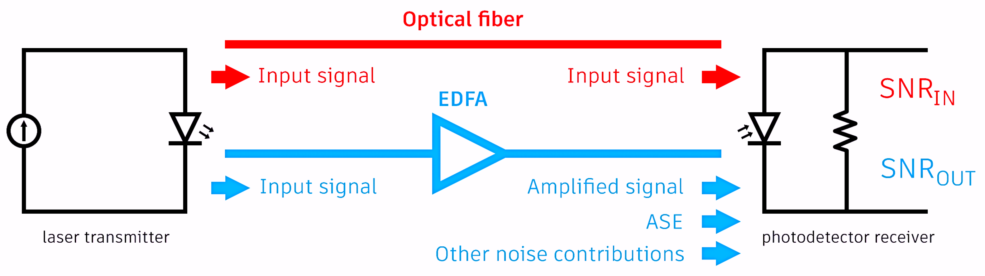
Figure 1.
Input and output SNR measurement setups for noise figure evaluation.
Figure 1.
Input and output SNR measurement setups for noise figure evaluation.
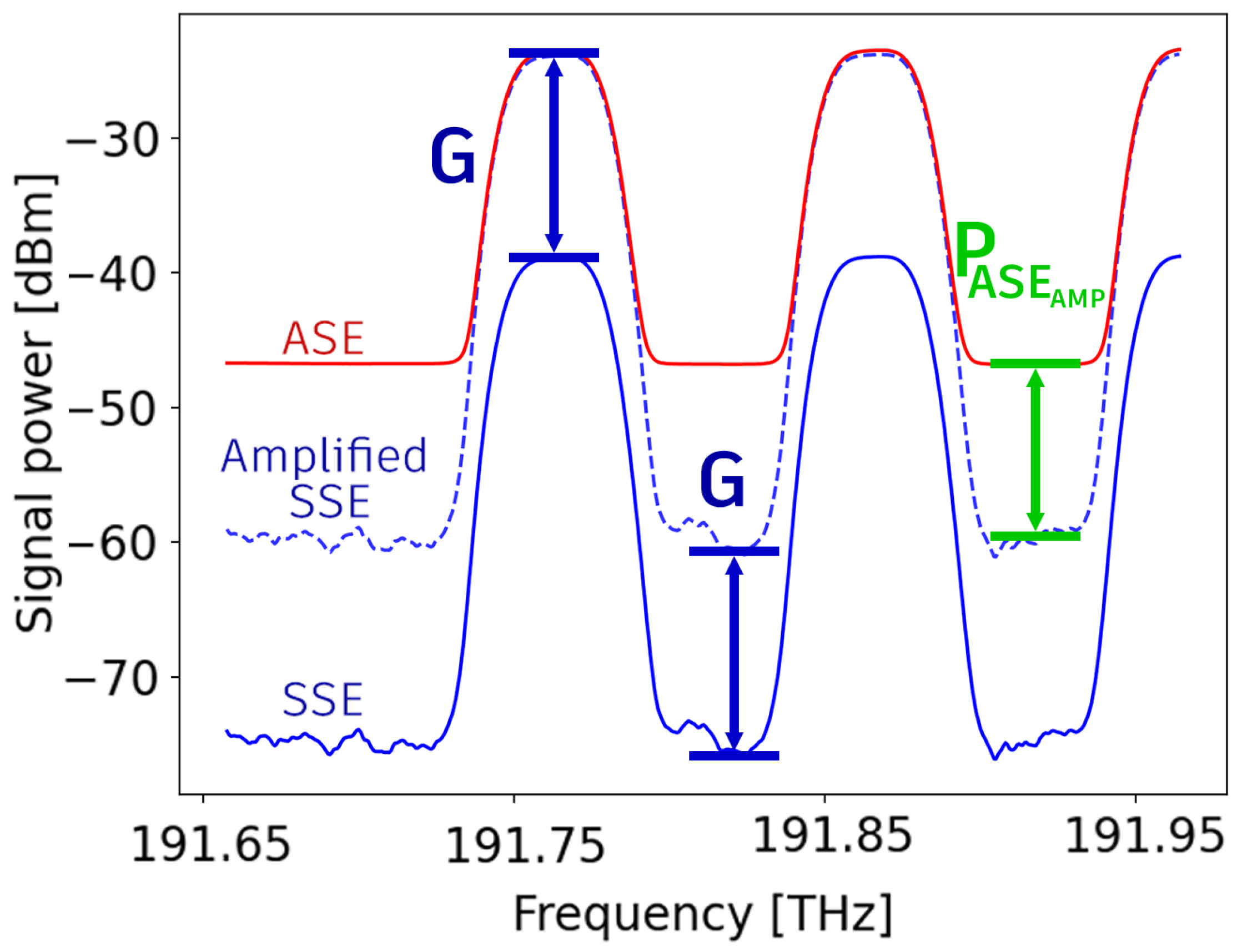
Figure 2.
Illustration of . The output spectrum (red) is shown alongside the input spectrum (blue) adjusted by the amplifier gain (blue dashed). represents the noise introduced by the EDFA to the amplified SSE level.
Figure 2.
Illustration of . The output spectrum (red) is shown alongside the input spectrum (blue) adjusted by the amplifier gain (blue dashed). represents the noise introduced by the EDFA to the amplified SSE level.
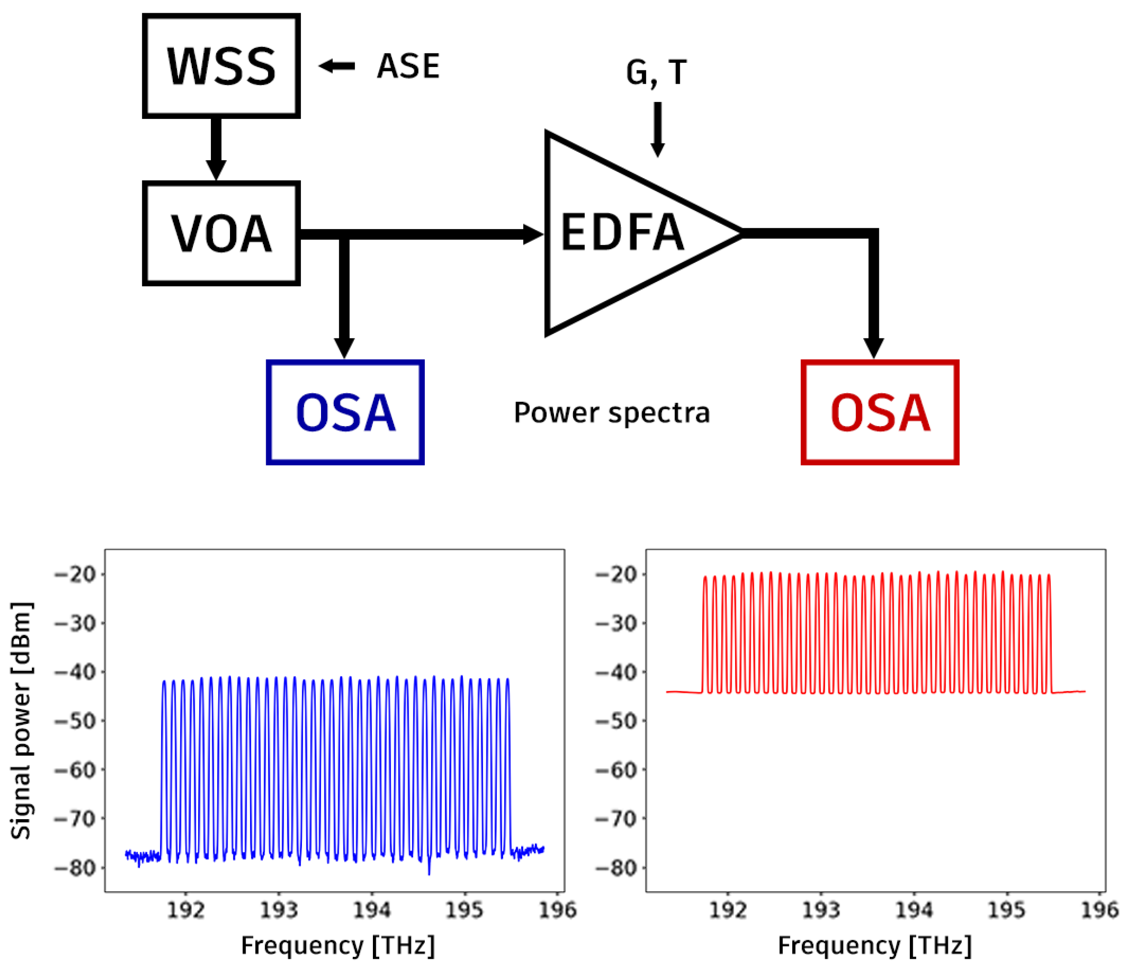
Figure 3.
Diagram of the test setup for measuring input (blue) and output (red) power spectral densities.
Figure 3.
Diagram of the test setup for measuring input (blue) and output (red) power spectral densities.
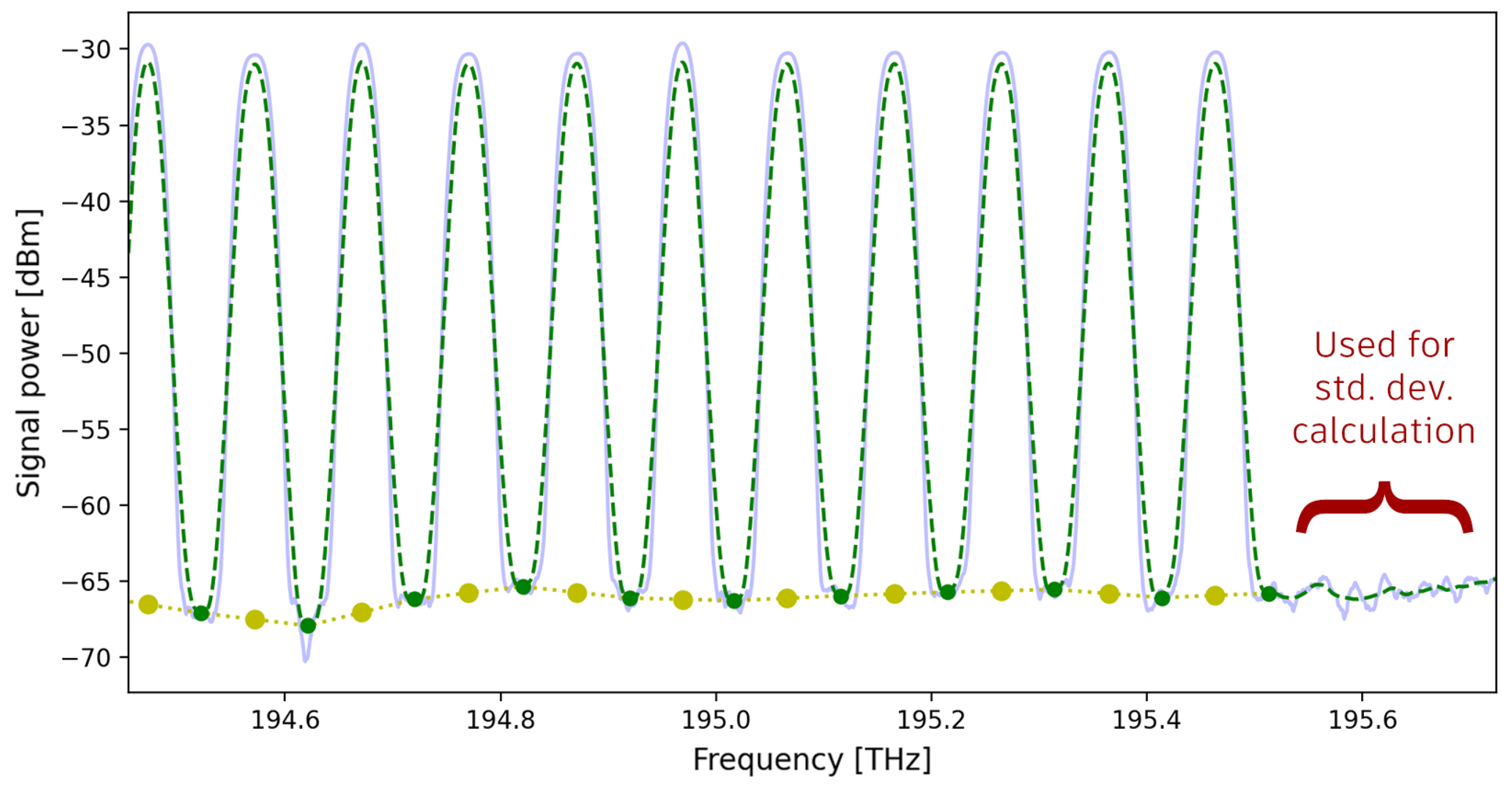
Figure 4.
Evaluation of SSE: The power density spectrum is convolved to obtain a smooth curve (green line). The middle points between two adjacent channels (green dots) are used for piecewise linear interpolation to evaluate the noise at the channel frequencies (yellow dots).
Figure 4.
Evaluation of SSE: The power density spectrum is convolved to obtain a smooth curve (green line). The middle points between two adjacent channels (green dots) are used for piecewise linear interpolation to evaluate the noise at the channel frequencies (yellow dots).
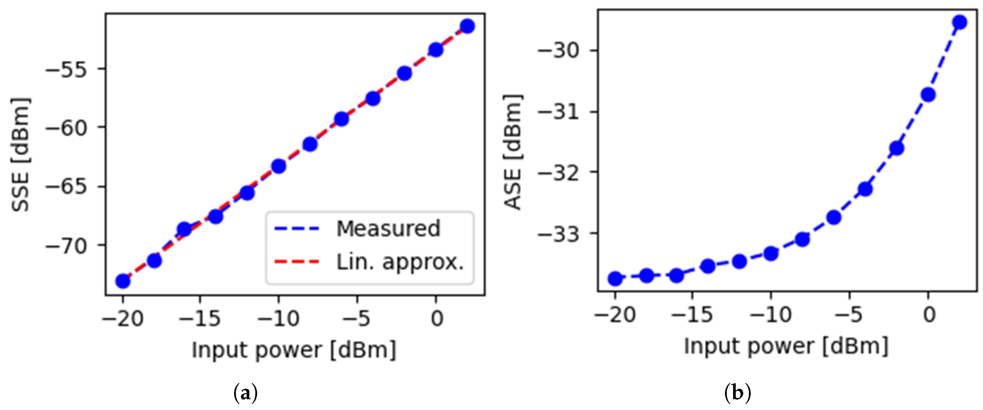
Figure 5.
Noise levels vs. input power for a commercial EDFA. (a) SSE; (b) ASE.
Figure 5.
Noise levels vs. input power for a commercial EDFA. (a) SSE; (b) ASE.
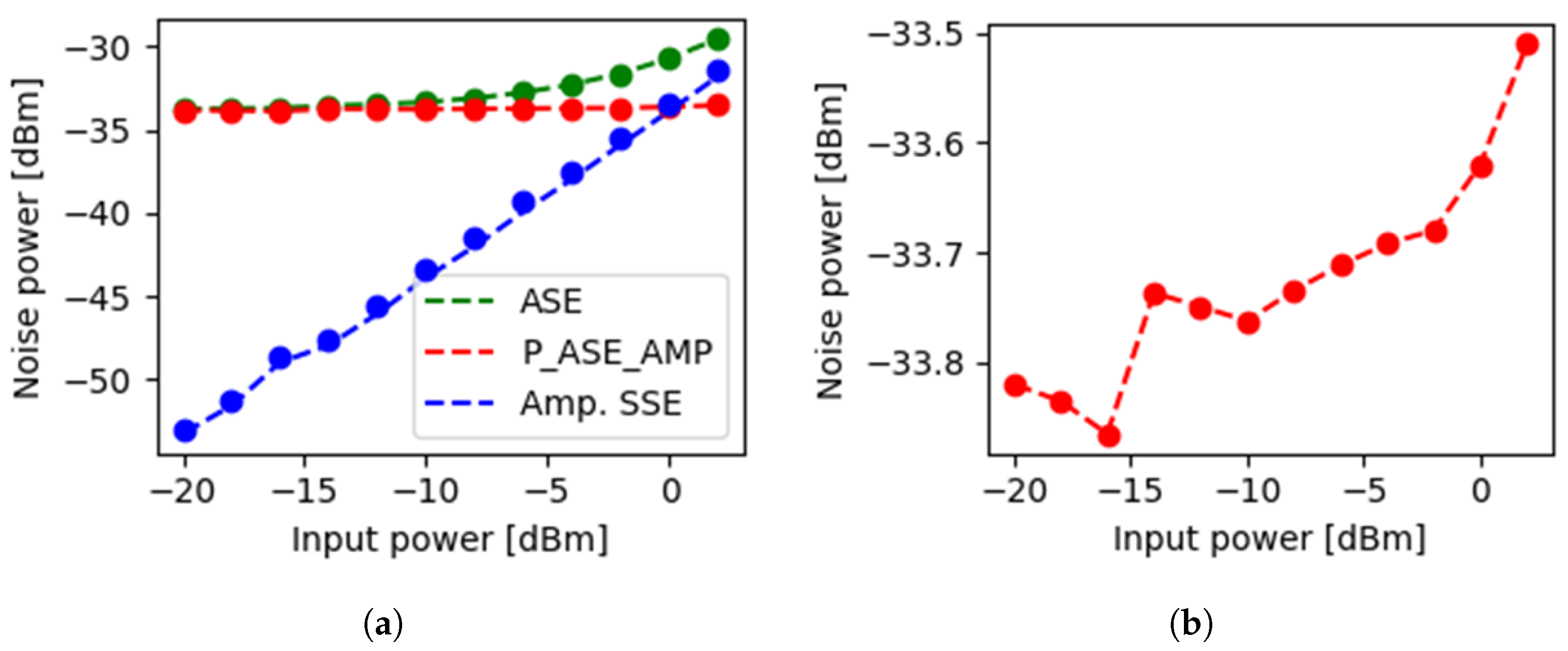
Figure 6.
vs. input power for a commercial EDFA. (a) , ASE and amplified SSE; (b) only.
Figure 6.
vs. input power for a commercial EDFA. (a) , ASE and amplified SSE; (b) only.
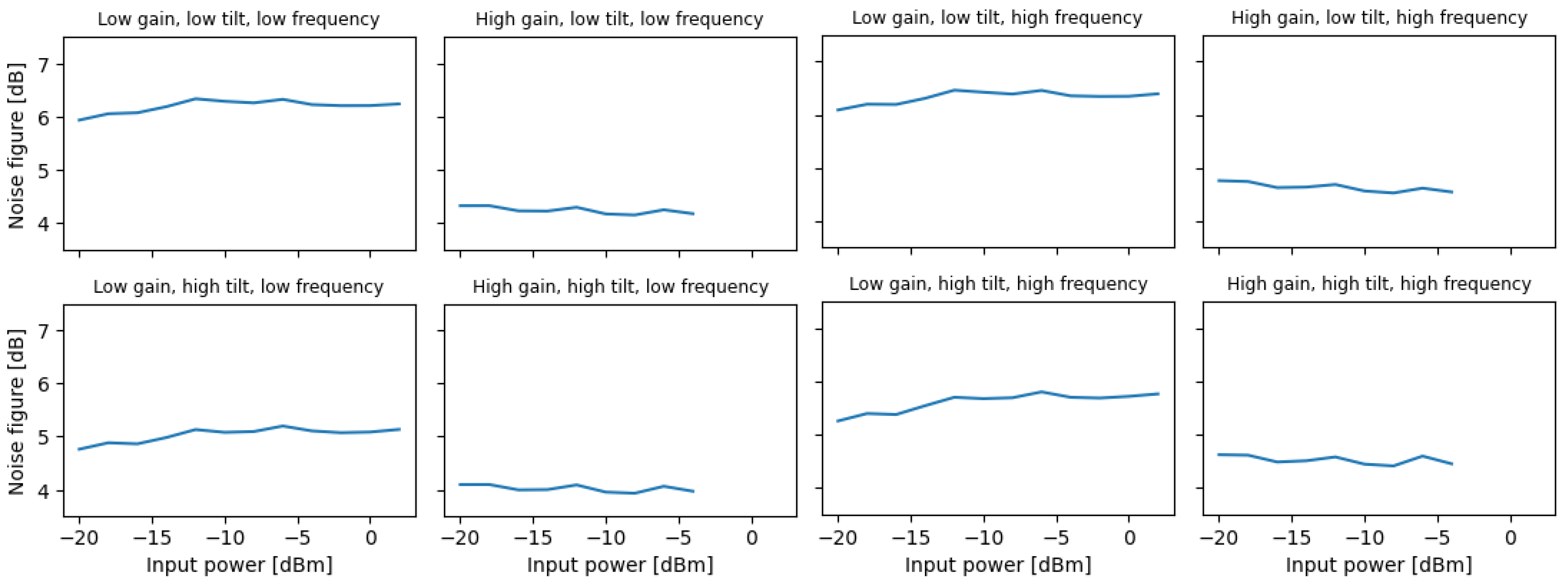
Figure 7.
Noise figure vs. input power, at various input parameter configurations.
Figure 7.
Noise figure vs. input power, at various input parameter configurations.
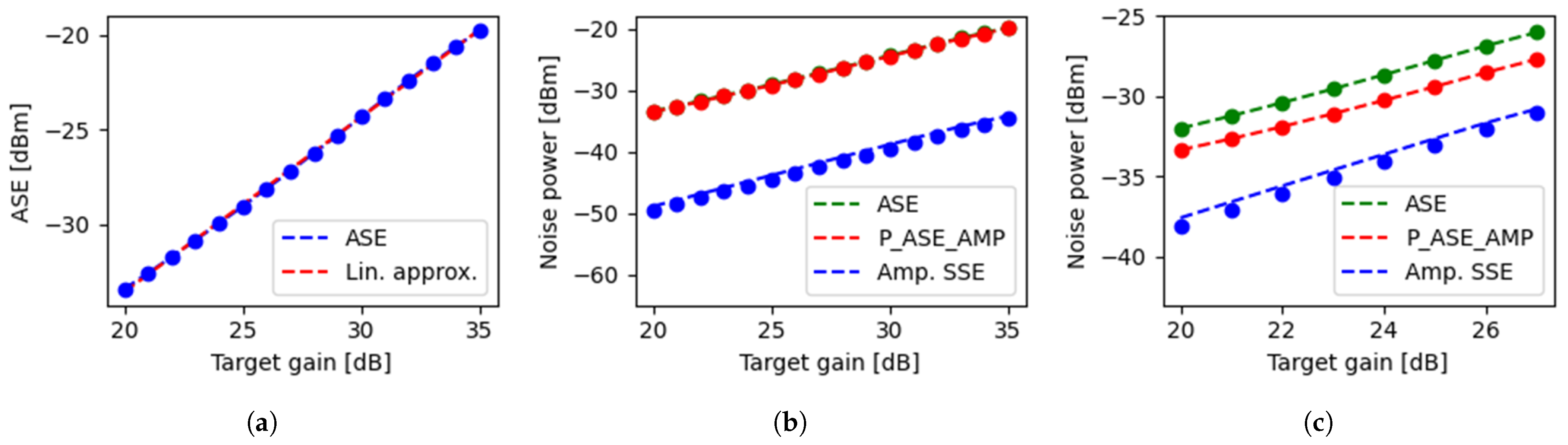
Figure 8.
(a) ASE vs. gain, with linear fitting; (b) vs. channel gain at low input power and (c) at high input power.
Figure 8.
(a) ASE vs. gain, with linear fitting; (b) vs. channel gain at low input power and (c) at high input power.
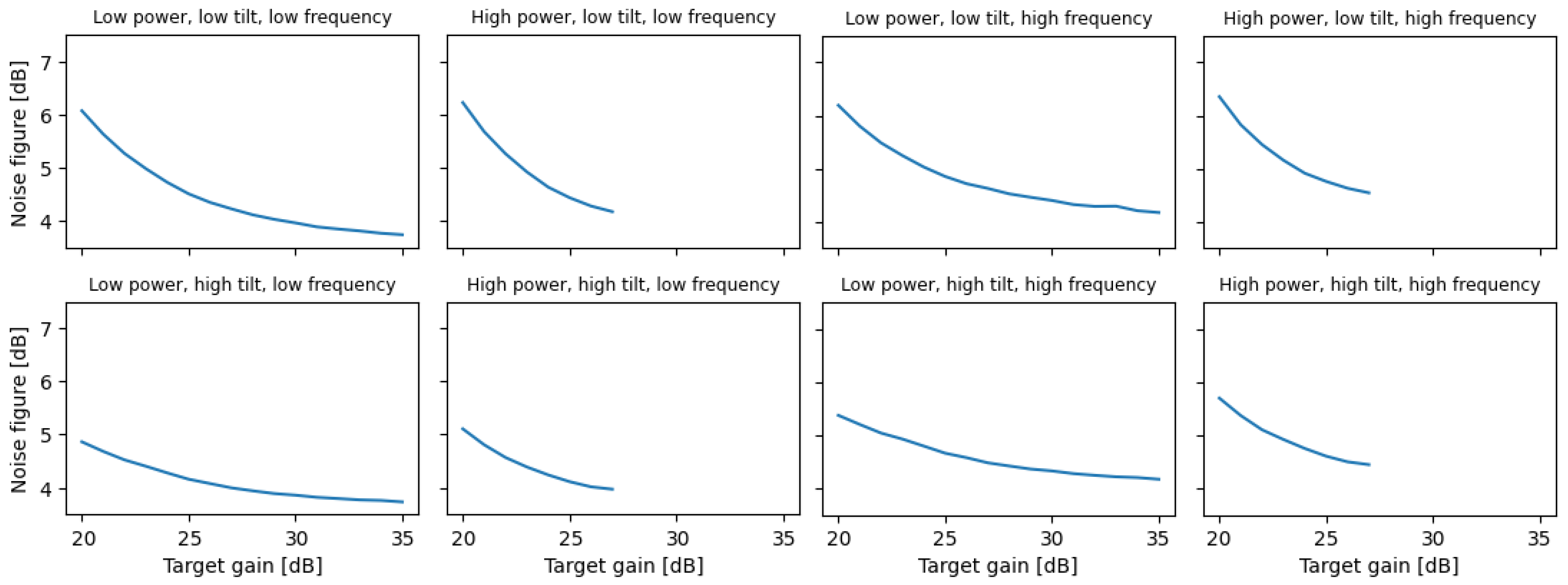
Figure 9.
Noise Figure vs. channel gain, at various input parameter configurations.
Figure 9.
Noise Figure vs. channel gain, at various input parameter configurations.
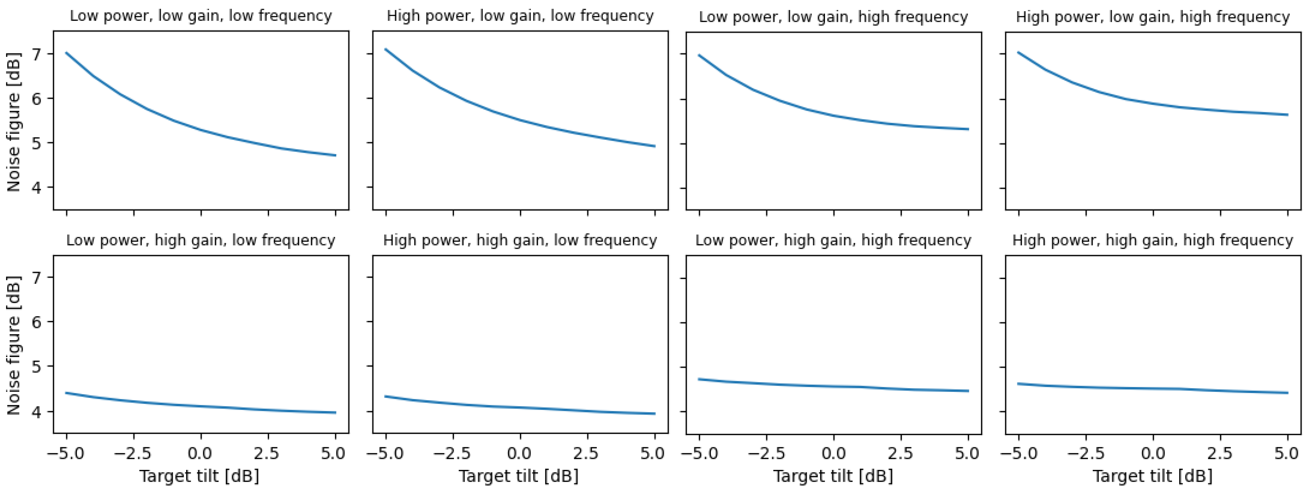
Figure 10.
Noise figure vs. target gain tilt, at various input parameter configurations.
Figure 10.
Noise figure vs. target gain tilt, at various input parameter configurations.
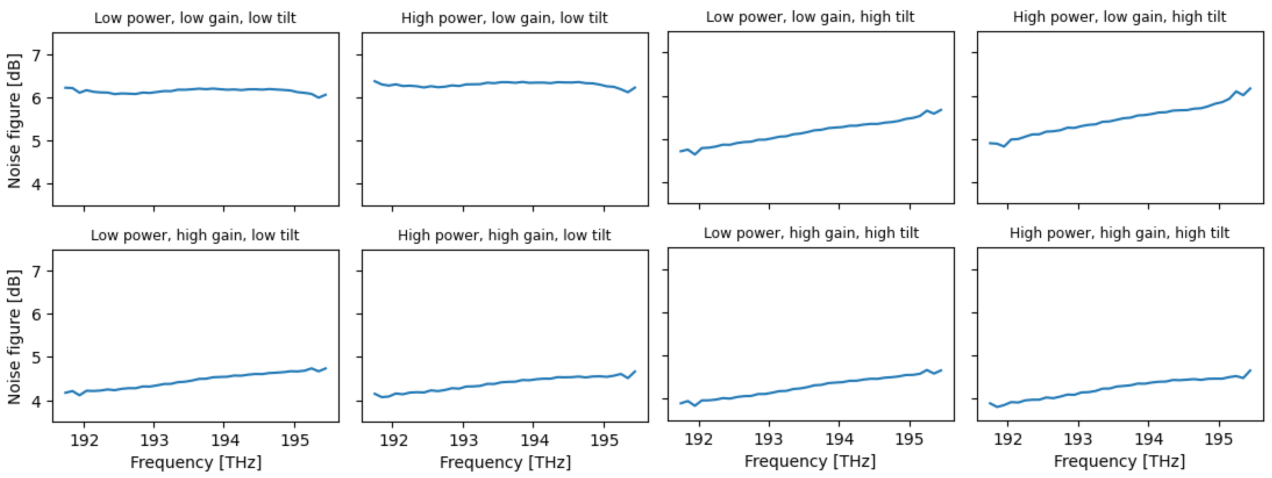
Figure 11.
Noise figure vs. channel frequency, at various input parameter configurations.
Figure 11.
Noise figure vs. channel frequency, at various input parameter configurations.
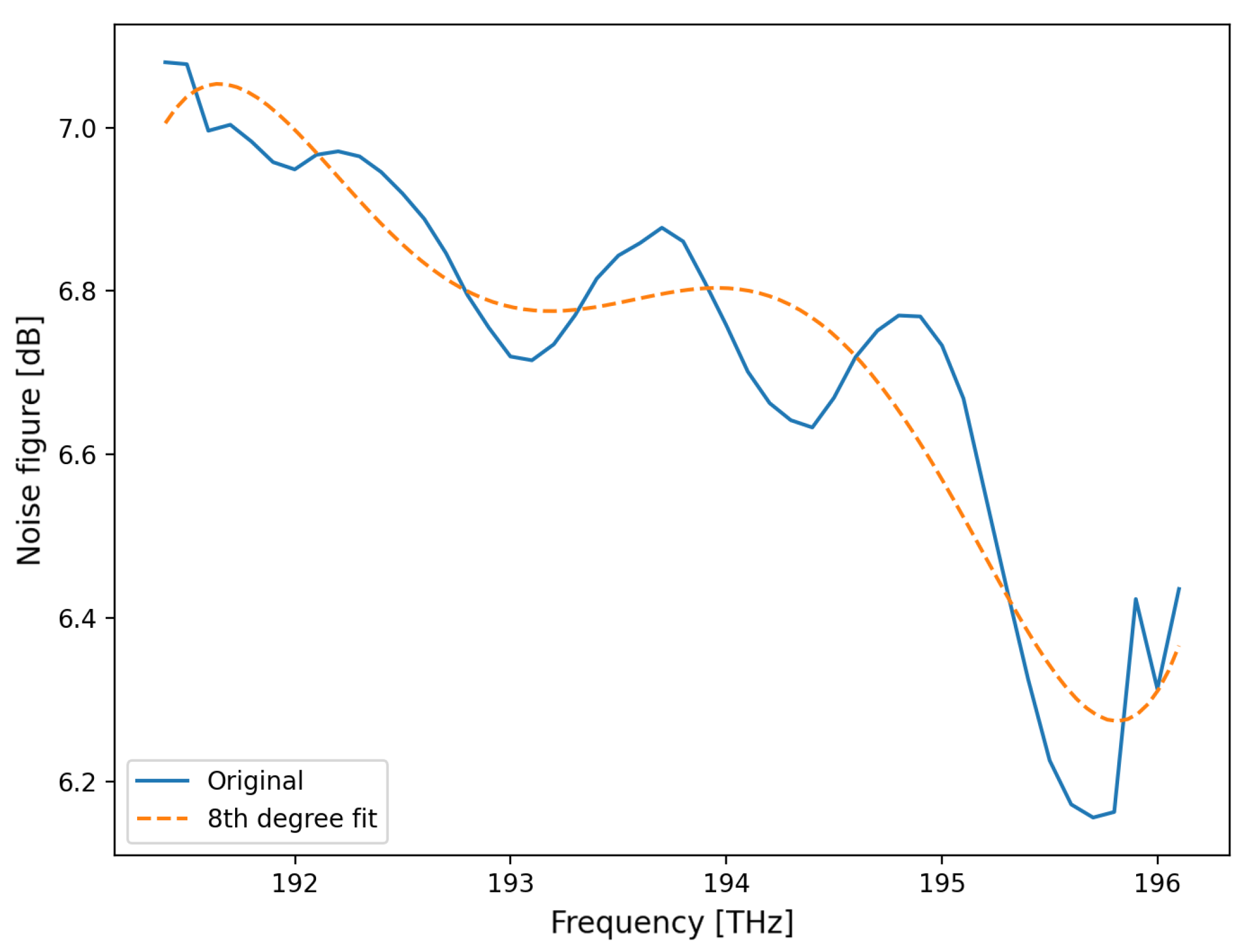
Figure 12.
An example of the significant variance in noise figure versus frequency under a worst-case scenario for a commercial EDFA.
Figure 12.
An example of the significant variance in noise figure versus frequency under a worst-case scenario for a commercial EDFA.
Figure 13.
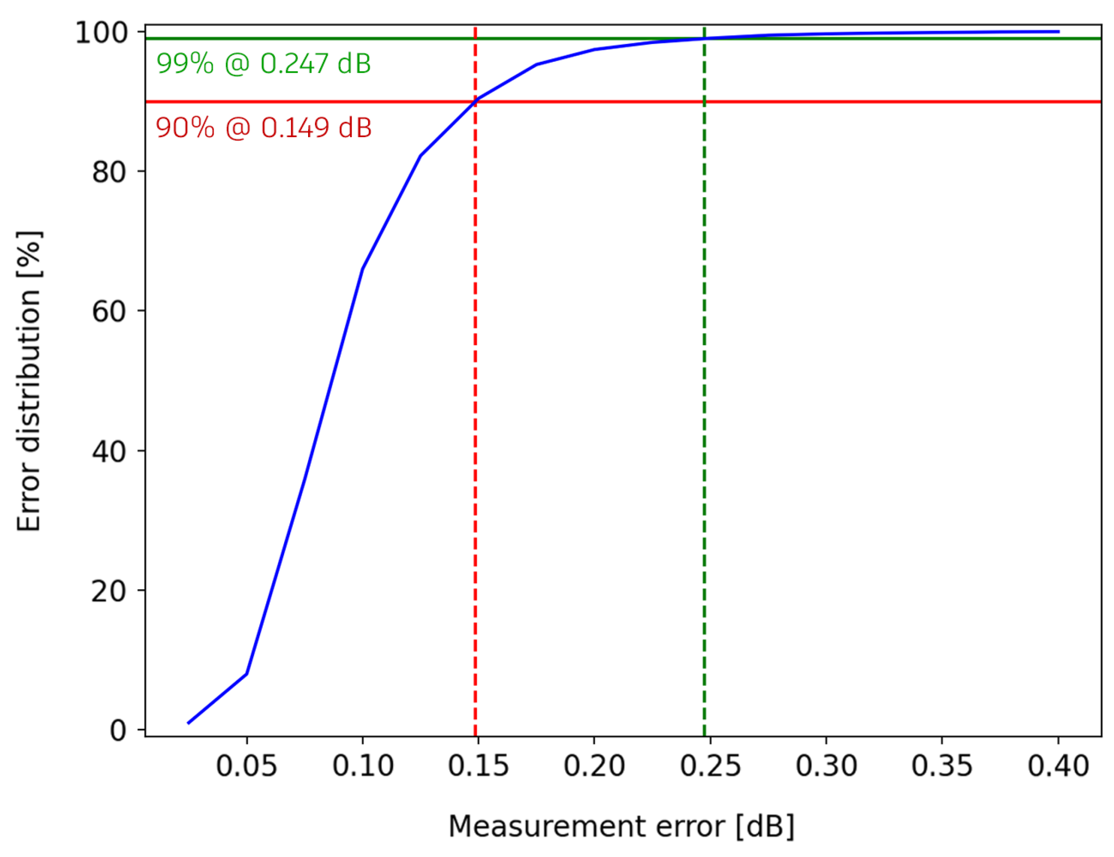
Cumulative distribution of measurement errors for Cisco EDFA-35 devices operating in the low-gain range (blue) and 90%-threshold (red), 99%-threshold (green) error values evaluation.
Figure 13.
Cumulative distribution of measurement errors for Cisco EDFA-35 devices operating in the low-gain range (blue) and 90%-threshold (red), 99%-threshold (green) error values evaluation.
Figure 14.
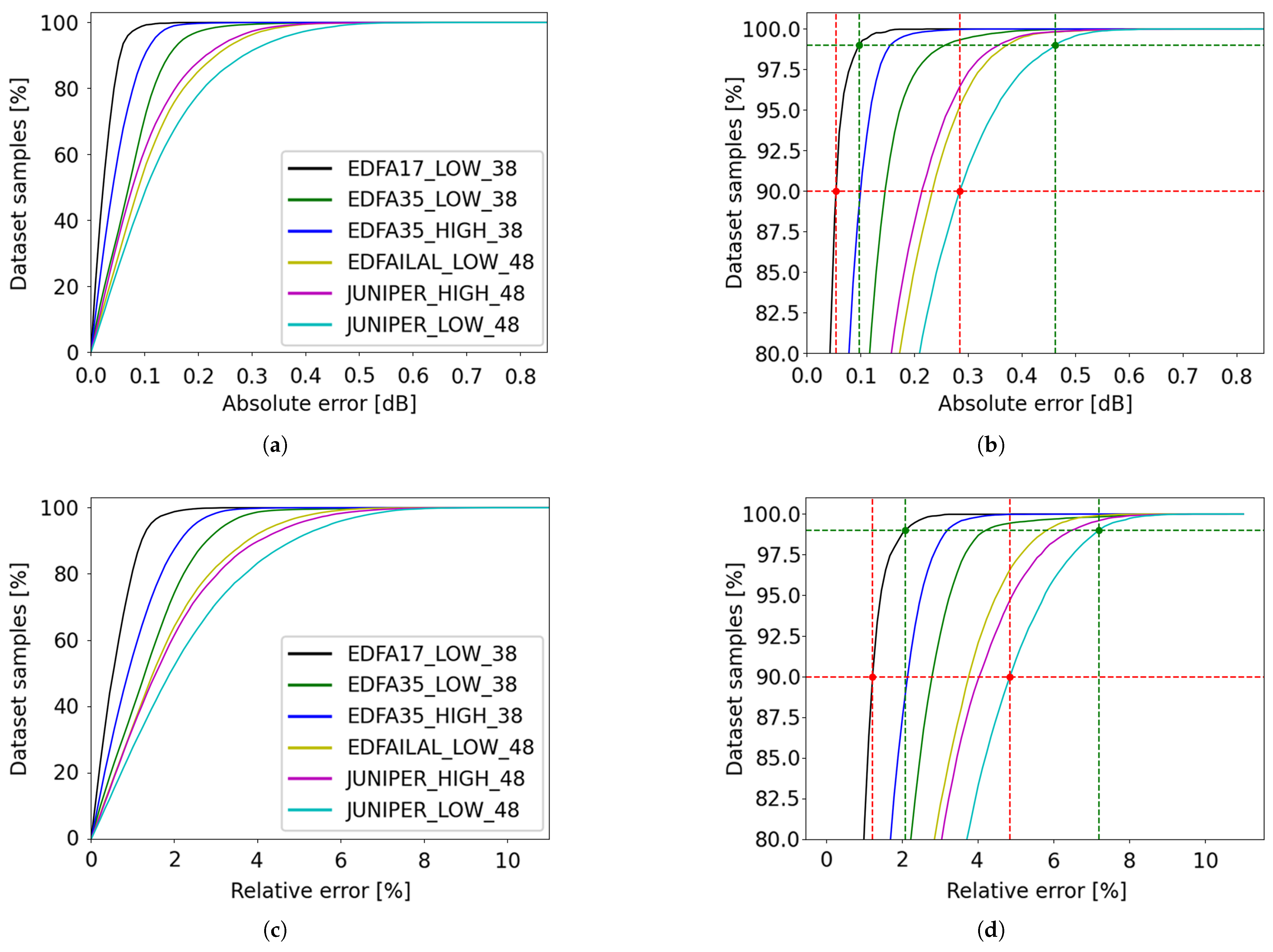
Cumulative distribution of absolute and relative errors of 70–30 split models. (a) Absolute errors; (b) Absolute errors, detail; (c) Relative errors; (d) Relative errors, detail. In (b,d) green and red dashed lines represent 99% and 90%-threshold values, respectively, with green and red bullets highlighting minimum and maximum values obtained through these curves.
Figure 14.
Cumulative distribution of absolute and relative errors of 70–30 split models. (a) Absolute errors; (b) Absolute errors, detail; (c) Relative errors; (d) Relative errors, detail. In (b,d) green and red dashed lines represent 99% and 90%-threshold values, respectively, with green and red bullets highlighting minimum and maximum values obtained through these curves.
Figure 15.
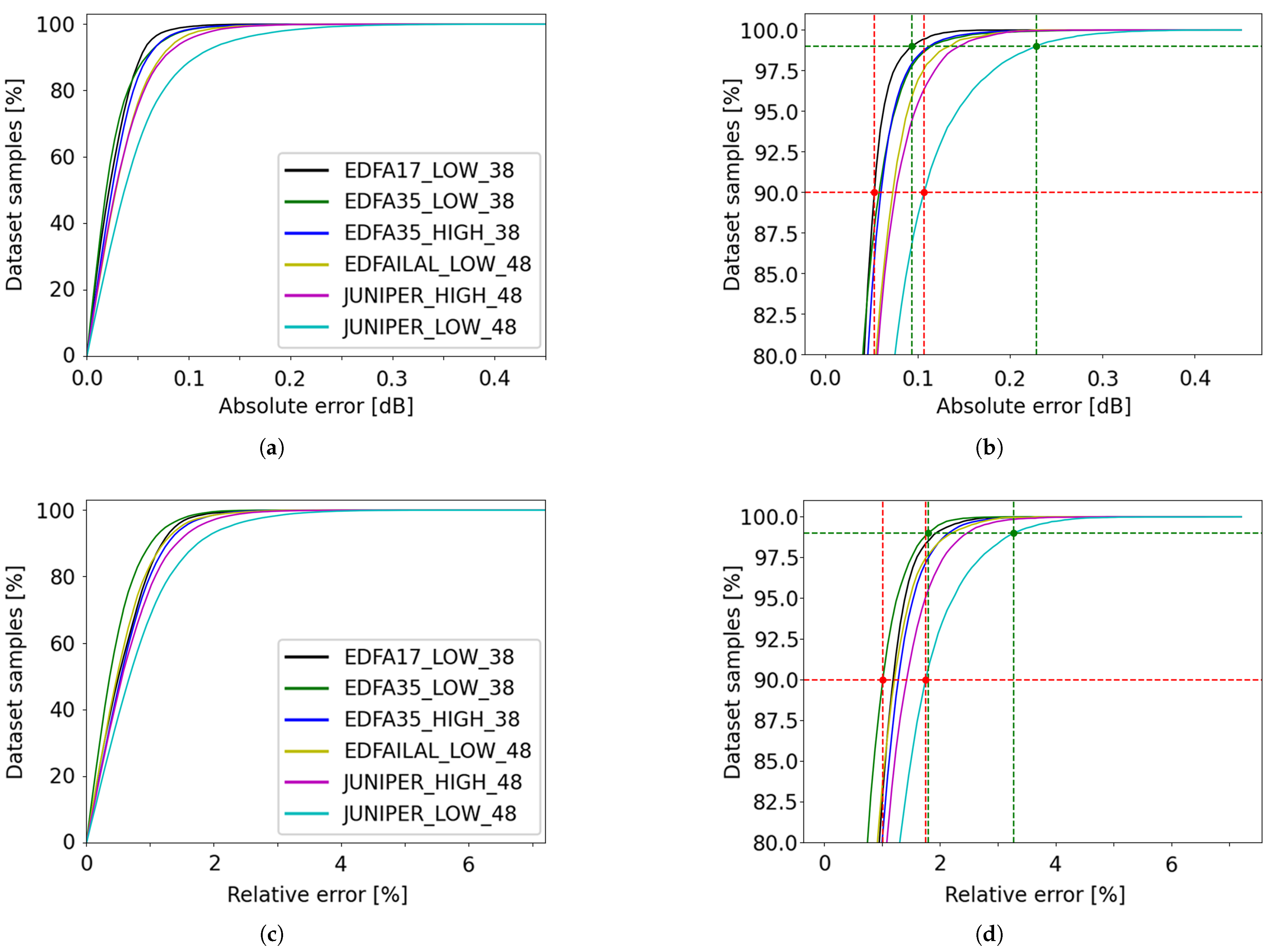
Cumulative distribution of absolute and relative errors of full dataset models. (a) Absolute errors; (b) Absolute errors, detail; (c) Relative errors; (d) Relative errors, detail. In (b,d) green and red dashed lines represent 99% and 90%-threshold values, respectively, with green and red bullets highlighting minimum and maximum values obtained through these curves.
Figure 15.
Cumulative distribution of absolute and relative errors of full dataset models. (a) Absolute errors; (b) Absolute errors, detail; (c) Relative errors; (d) Relative errors, detail. In (b,d) green and red dashed lines represent 99% and 90%-threshold values, respectively, with green and red bullets highlighting minimum and maximum values obtained through these curves.
Figure 16.
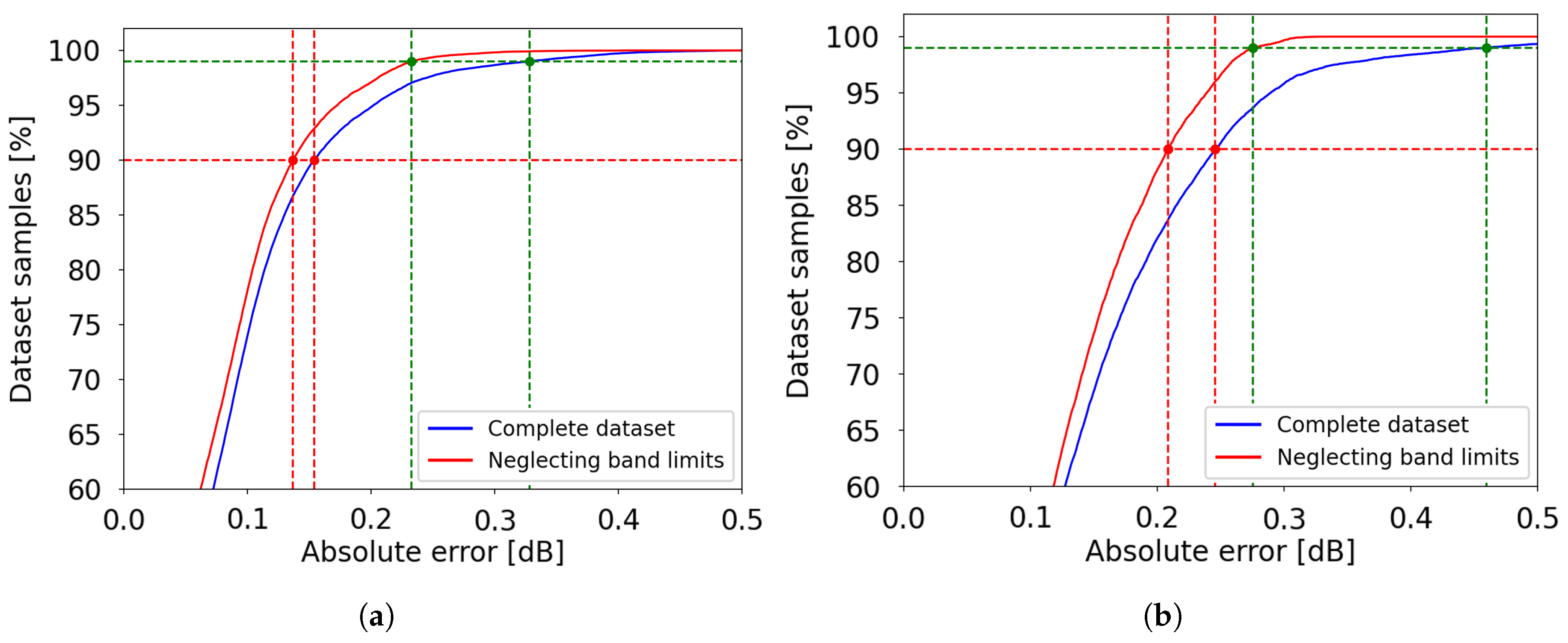
Cumulative distribution of absolute errors and their correlation with the frequency range. (a) EDFA-35, low-gain range; (b) L-band EDFA, low-gain range. Green and red dashed lines represent 99% and 90%-threshold values, respectively, with green and red bullets highlighting minimum and maximum values obtained through these curves.
Figure 16.
Cumulative distribution of absolute errors and their correlation with the frequency range. (a) EDFA-35, low-gain range; (b) L-band EDFA, low-gain range. Green and red dashed lines represent 99% and 90%-threshold values, respectively, with green and red bullets highlighting minimum and maximum values obtained through these curves.
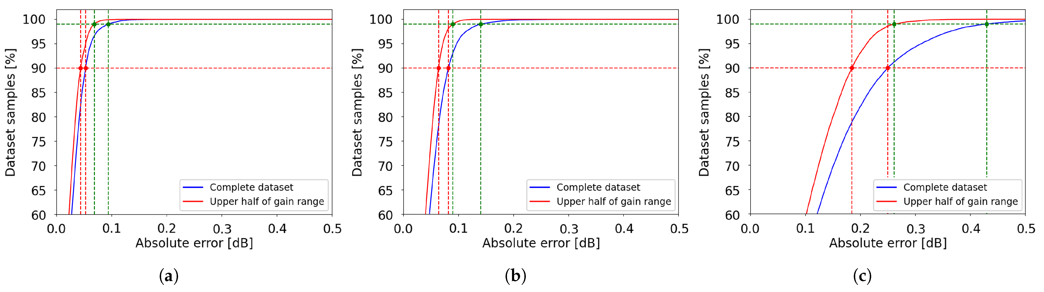
Figure 17.
Cumulative distribution of absolute errors and their correlation with gain and tilt range: (a) EDFA-17, low-gain range; (b) EDFA-35, high-gain range; (c) Juniper, low-gain range. Green and red dashed lines represent 99% and 90%-threshold values, respectively, with green and red bullets highlighting minimum and maximum values obtained through these curves.
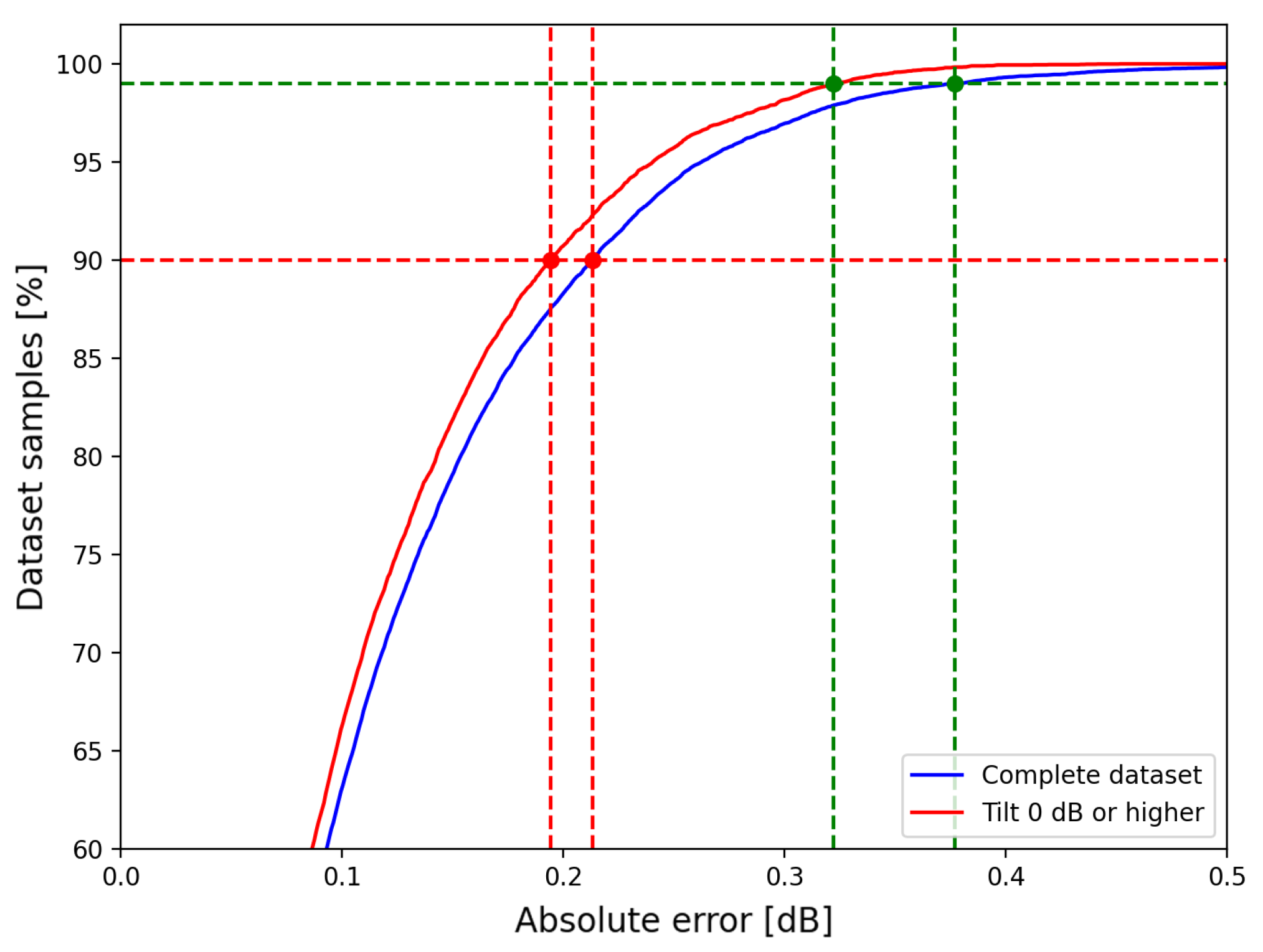
Figure 18.
Correlation between tilt range and error reduction in JUNIPER devices. Green and red dashed lines represent 99% and 90%-threshold values, respectively, with green and red bullets highlighting minimum and maximum values obtained through these curves.
Figure 18.
Correlation between tilt range and error reduction in JUNIPER devices. Green and red dashed lines represent 99% and 90%-threshold values, respectively, with green and red bullets highlighting minimum and maximum values obtained through these curves.
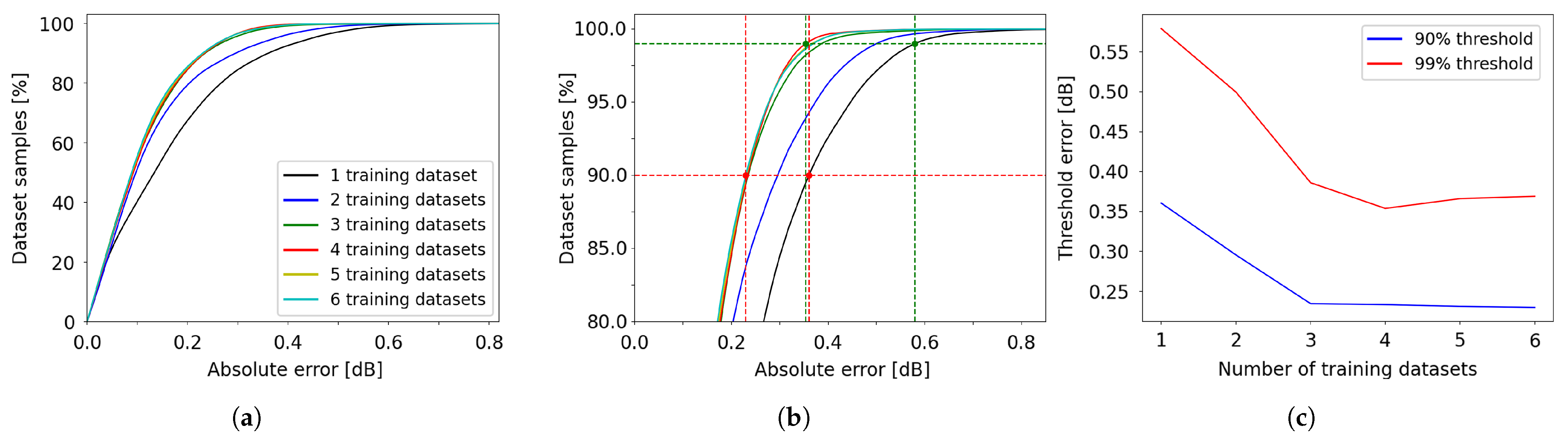
Figure 19.
Cumulative distribution of the absolute error for the L-band EDFA device, as a function of the number of training datasets. (a) Overview of absolute errors; (b) Zoomed-in view of the y-axis region between 80% and 100%; (c) 90% and 99% error thresholds versus the number of datasets.
Figure 19.
Cumulative distribution of the absolute error for the L-band EDFA device, as a function of the number of training datasets. (a) Overview of absolute errors; (b) Zoomed-in view of the y-axis region between 80% and 100%; (c) 90% and 99% error thresholds versus the number of datasets.
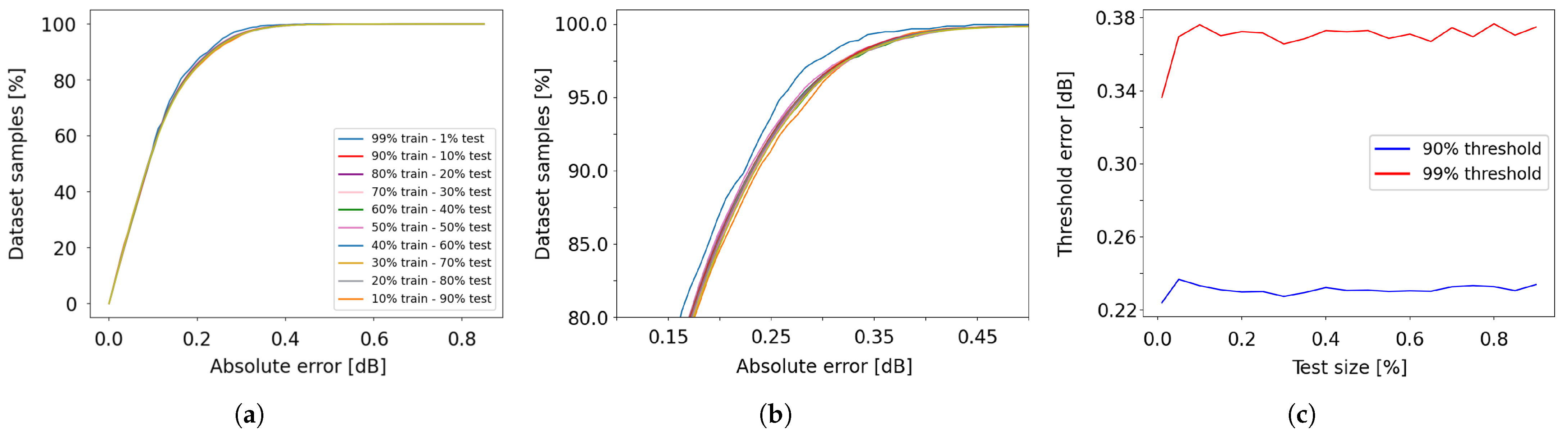
Figure 20.
Cumulative distribution of the absolute error for the L-band EDFA device, as a function of the train/test split ratio. (a) Overview of absolute errors; (b) Zoomed-in view of the y-axis region between 80% and 100%; (c) 90% and 99% error thresholds versus test size.
Figure 20.
Cumulative distribution of the absolute error for the L-band EDFA device, as a function of the train/test split ratio. (a) Overview of absolute errors; (b) Zoomed-in view of the y-axis region between 80% and 100%; (c) 90% and 99% error thresholds versus test size.
Table 1.
Computation time to compute the noise figure for each EDFA dataset.
Table 1.
Computation time to compute the noise figure for each EDFA dataset.
| Device | Gain | Dataset No. | Time [s] | Row Count | Time per Row [ms] |
|---|
| EDFA-17 | LOW | 1 | 13.22 | 21,318 | 0.62 |
| EDFA-35 | HIGH | 1 | 32.95 | 56,848 | 0.58 |
| EDFA-35 | HIGH | 2 | 31.99 | 56,848 | 0.56 |
| EDFA-35 | LOW | 1 | 25.79 | 45,144 | 0.57 |
| EDFA-35 | LOW | 2 | 27.77 | 46,816 | 0.59 |
| EDFA-35 | LOW | 3 | 25.77 | 45,144 | 0.57 |
| EDFA-35 | LOW | 4 | 34.54 | 58,608 | 0.59 |
| EDFA-ILA-L | LOW | 1 | 12.08 | 21,360 | 0.57 |
| EDFA-ILA-L | LOW | 2 | 12.52 | 21,360 | 0.59 |
| EDFA-ILA-L | LOW | 3 | 9.03 | 14,976 | 0.60 |
| EDFA-ILA-L | LOW | 4 | 9.16 | 14,976 | 0.61 |
| EDFA-ILA-L | LOW | 5 | 8.83 | 14,976 | 0.59 |
| EDFA-ILA-L | LOW | 6 | 8.66 | 14,976 | 0.58 |
| JUNIPER | HIGH | 1 | 10.79 | 18,816 | 0.57 |
| JUNIPER | HIGH | 2 | 11.44 | 18,816 | 0.61 |
| JUNIPER | HIGH | 3 | 12.15 | 18,816 | 0.65 |
| JUNIPER | HIGH | 4 | 11.06 | 18,480 | 0.60 |
| JUNIPER | LOW | 1 | 16.15 | 29,232 | 0.55 |
| JUNIPER | LOW | 2 | 16.70 | 29,232 | 0.57 |
| JUNIPER | LOW | 3 | 17.23 | 29,232 | 0.59 |
| JUNIPER | LOW | 4 | 16.90 | 29,232 | 0.58 |
Table 2.
Computation time for training the noise figure polynomial models.
Table 2.
Computation time for training the noise figure polynomial models.
| Device | Gain | Time [s] | Total Row Count | Time per Row [ms] |
|---|
| EDFA-17 | LOW | 2.70 | 21,318 | 0.13 |
| EDFA-35 | HIGH | 15.04 | 113,696 | 0.13 |
| EDFA-35 | LOW | 35.08 | 195,712 | 0.18 |
| EDFA-ILA-L | LOW | 16.58 | 102,624 | 0.16 |
| JUNIPER | HIGH | 12.05 | 74,928 | 0.16 |
| JUNIPER | LOW | 17.83 | 116,928 | 0.15 |
Table 3.
Execution time of the model evaluation Python class, categorized by function.
Table 3.
Execution time of the model evaluation Python class, categorized by function.
| Class Method(s) | Exec. Time [ms] | Exec. Time [s] | Exec. Time [ns] |
|---|
| Initialization | 40.76 | 40,759.31 | 40,759,306.60 |
| NF evaluation (single) | 0.05 | 47.60 | 47,600.11 |
| NF evaluation (array) | <0.01 | 0.61 | 613.81 |
Table 4.
Execution time of the array estimation function for the noise figure, as a function of array length.
Table 4.
Execution time of the array estimation function for the noise figure, as a function of array length.
| Array Length | Exec. Time per Sample [s] |
|---|
| 1 | 1479.72 |
| 2 | 746.99 |
| 5 | 298.97 |
| 10 | 150.46 |
| 20 | 76.76 |
| 33 | 47.39 |
Table 5.
Performance of deep-learning EDFA model, maximum absolute error [dB].
Table 5.
Performance of deep-learning EDFA model, maximum absolute error [dB].
| Case | EDFA 1 | EDFA 2 | EDFA 3 | EDFA 4 | EDFA 5 | EDFA 6 | EDFA 7 |
|---|
| Fixed NF | 1.3914 | 1.1150 | 0.3941 | 0.4304 | 0.4176 | 0.5063 | 0.5245 |
| Model NF | 1.3099 | 1.1103 | 0.3730 | 0.4461 | 0.4067 | 0.4881 | 0.5351 |
| | | | | | | | |
Table 6.
Performance of deep-learning EDFA model, mean absolute error [dB].
Table 6.
Performance of deep-learning EDFA model, mean absolute error [dB].
| Case | EDFA 1 | EDFA 2 | EDFA 3 | EDFA 4 | EDFA 5 | EDFA 6 | EDFA 7 |
|---|
| Fixed NF | 0.1269 | 0.0849 | 0.0583 | 0.0590 | 0.0566 | 0.0587 | 0.0771 |
| Model NF | 0.1093 | 0.0816 | 0.0543 | 0.0596 | 0.0555 | 0.0625 | 0.0772 |
| | | | | | | | |
Table 7.
Performance of deep-learning EDFA model, adjusted score [%].
Table 7.
Performance of deep-learning EDFA model, adjusted score [%].
| Case | EDFA 1 | EDFA 2 | EDFA 3 | EDFA 4 | EDFA 5 | EDFA 6 | EDFA 7 |
|---|
| Fixed NF | 92.2129 | 95.3613 | 95.9068 | 97.7005 | 91.6659 | 94.8887 | 93.1631 |
| Model NF | 89.3877 | 95.2287 | 96.0442 | 97.5909 | 91.9185 | 94.2216 | 93.5089 |
| | | | | | | | |
Table 8.
Performance of deep-learning EDFA model, RMSE [dB].
Table 8.
Performance of deep-learning EDFA model, RMSE [dB].
| Case | EDFA 1 | EDFA 2 | EDFA 3 | EDFA 4 | EDFA 5 | EDFA 6 | EDFA 7 |
|---|
| Fixed NF | 0.1908 | 0.1413 | 0.0810 | 0.0813 | 0.0782 | 0.0828 | 0.1093 |
| Model NF | 0.1715 | 0.1390 | 0.0773 | 0.0828 | 0.0758 | 0.0885 | 0.1081 |
| | | | | | | | |


