Relaxation Modeling of Unidirectional Carbon Fiber Reinforced Polymer Composites Before and After UV-C Exposure

Abstract

Carbon fiber-reinforced polymers (CFRPs) are widely used in aerospace for their lightweight and high-performance characteristics. This study examines the long-term viscoelastic behavior of CFRP after UV-C exposure, simulating low Earth orbit conditions. The viscoelastic properties of the polymer were evaluated using dynamic mechanical analysis and the time-temperature superposition principle on both unexposed and UV-C-exposed samples. After UV-C exposure, the polymer’s instantaneous modulus decreased by about $15\%$. Over a 32-year period, the modulus of the unexposed resin is expected to degrade to approximately $25\%$ of its initial value, while the exposed resin drops to around $15\%$. These experimental results were incorporated into finite element method models of a unidirectional CFRP representative volume element. The simulations showed that UV-C exposure caused only a slight reduction in the CFRP’s axial relaxation coefficient along the fiber’s axis, with no significant time-dependent degradation, as the fiber dominates this behavior. In contrast, the axial relaxation coefficient perpendicular to the fiber’s axis, as well as the off-diagonal and shear relaxation coefficients, showed more notable changes, with an approximate $10\%$ reduction in their initial values after UV-C exposure. Over 32 years, degradation became much more severe, with differences between the pre- and post-exposure coefficient values reaching up to nearly $60\%$.

1. Introduction

Carbon fiber-reinforced polymers (CFRPs) have become a cornerstone in aerospace engineering due to their lightweight and high specific mechanical properties. As these materials are increasingly employed in critical aerospace applications, understanding their performance under the extreme conditions of space is essential. The space environment is far from empty; exposure to its harsh, inhospitable, and potentially hazardous conditions can be detrimental to CFRPs used in aerospace applications [1]. Specifically, in low Earth orbit (LEO), there are various potential sources of damage that can be fatal for polymers and consequently for all polymer matrix composites (PMCs), including CFRPs [2,3]. In fact, research from in-flight exposure experiments has shown that the harsh conditions in LEO environment can lead to erosion, mass loss, and degradation of properties of polymers and PMC materials [4,5,6].

The LEO environment is characterized by ultra-high vacuum conditions, generally below ${10}^{-5}$ Torr. Such high vacuum conditions can lead to outgassing of the polymer matrix [7]. In LEO environment, spacecraft are exposed to UV-C radiation, which can rapidly accelerate degradation processes in polymeric materials [8]. Given the satellite’s orbital velocity of approximately 8 km/s in LEO, it is exposed to a highly energetic stream of atomic oxygen (AO) with an energy of about 5 eV, which can cause surface erosion and degrade the mechanical properties of polymer composites [9,10,11]. Thermal cycling in LEO, with temperatures from $-150$ °C to $150$ °C, can induce microcracks in polymer composites due to differential thermal expansion between the fiber and matrix [12]. Furthermore, the LEO environment is exposed to charged particles, electromagnetic radiation, micrometeoroids, and human-made debris, all of which can further contribute to material degradation. Therefore, understanding the mechanical properties of polymers and PMCs in LEO is essential. This study examines the impact of UV irradiation, which significantly deteriorates the performance of CFRPs [13].

Significant research has been dedicated to understanding the effects of UV radiation on polymeric materials. The study conducted by Singh and Sharma explores the degradation mechanisms that polymers can undergo, including photo-oxidation, where UV radiation has sufficient energy to cleave chemical bonds in polymer chains, generating free radicals. These radicals react with oxygen, leading to material degradation through mechanisms such as chain scission and cross-linking [14]. This degradation notably impacts the mechanical properties of polymeric materials [15]. In recent years, a focus has been the implication of UV exposure on CFRPs. Experimental characterization on both unexposed and exposed CFRPs have shown that UV aging generally degrades their properties [16,17]. Similar studies conducted on CFRPs made from recycled carbon fibers have observed the same trends [18]. Additionally, research effort has been devoted toward enhancing the performance of CFRPs using multi walled nanotubes (MWNTs) and thin-ply to mitigate the effect of UV exposure [19]. However, the long-term performance of CFRP after UV exposure environment remains largely unexplored, with only a few studies addressing this issue [20,21]. To gain valuable insights into the long-term behavior of CFRP in the LEO environment, our study focuses on characterizing its viscoelastic properties over an extended period following exposure to UV-C radiation dose equivalent to one year in LEO conditions.

To do so, the long-term viscoelastic behavior of an aerospace-grade epoxy resin system is firstly characterized, both prior and after exposure to a UV-C radiation dose equivalent to one year in LEO. At this extent, our work involves the construction of a master curve, i.e., a continuous representation of the material’s viscoelastic properties over a broad range of frequencies. For this purpose, short-duration tests using dynamic mechanical analysis (DMA) are conducted, and the time–temperature superposition principle (TTSP) is subsequently applied. The TTSP is based on the idea that changes in deformation rate can be equivalently represented as changes in temperature, enabling the extrapolation of long-term material behavior from short-duration tests conducted at various temperatures. This principle has been extensively utilized to evaluate the long-term behavior of epoxy resins [22,23,24,25,26]. In our work, master curves are constructed for the epoxy resin system both in its pristine state and after exposure to UV-C radiation. The pristine state serves as a baseline for comparison, while the UV-C exposed state allows us to quantify the impact of UV-C radiation on the polymer’s viscoelastic properties.

To extend the insights gained from the epoxy resin system to CFRP, it is essential to use suitable functions to fit the viscoealstic experimental data of the polymer. These functions can then be applied in future modeling efforts. A widely used function is the so called Prony series expansion. The literature shows different approaches to determine the Prony Series coefficients starting from experimental data [27,28,29,30,31,32,33,34,35,36,37,38,39,40,41,42,43]. Many of these approaches employ deterministic strategies that can only find locally optimal solutions by moving from one point to another within the search space. For instance, methods such as the multidata approach [27] and its enhanced versions [37,38] use linear least squares solvers (LLSS), while simplifying the problem often results in a ‘secondary-optimal’. Other methods have employed nonlinear least squares solvers [41,42]. However, these methods can suffer from ill-conditioning and divergence if the initial estimates are significantly off. To overcome the limitation of these traditional optimization techniques, Cui and Brinson proposed a two-step method combining a LLSS with particle swarm optimization (PSO). The use of the PSO, which is a stochastic optimization algorithm, broadens the search space of the LLSS and improves its chances of finding a global optimal solution [44]. In this work, the approach proposed by Cui and Brinson is applied, which has proven effective in various cases, to determine the Prony series coefficients that best fit the experimentally constructed master curves.

After determining the Prony series coefficients that describe the viscoelastic behavior of the polymer, these properties can be incorporated into finite element method (FEM) models to predict the behavior of CFRP materials. A common modeling approach in the literature for CFRP material involves constructing a representative volume element (RVE) and applying homogenization techniques. RVE approach and homogenization technique have been used for decades to predict the elastic properties of unidirectional (UD) CFRP through finite element (FE) software [45,46,47]. In recent years, many RVE models have also been developed to evaluate the viscoelastic properties of UD CFRP materials [48,49,50,51,52]. This approach has not yet been applied to predict the viscoelastic behavior of UD CFRP accounting for exposure to UV-C radiation. In this study, its potential for this specific application is explored.

This paper is organized as follows. First, the materials under investigation are presented and the manufacturing and conditioning processes are described. Then, the methodology for characterizing viscoelastic properties of the epoxy resin system are detailed and the approach used for fitting the experimental data to a Prony series expansion is outlined. Subsequently, the FEM modeling process for the UD CFRP material is described. Results for all stages of this work are presented and discussed. Finally, conclusions are drawn.

2. Materials

This section presents the materials involved in this study, which are unidirectional (UD) carbon fiber reinforced polymer (CFRP) composite materials.

The carbon fiber (CF) used as the reinforcement phase in the composite under investigation is the standard modulus Torayca^® T300 fiber. The matrix phase is an aerospace-grade resin system, CYCOM^® 823 RTM. The preparation of the resin-only specimens and their conditioning to simulate exposure to the equivalent UV-C dose experienced in one year in LEO orbit is detailed in the following subsection.

Resin-Only Specimen Preparation and Conditioning

Resin-only specimens were manufactured using the aerospace-grade thermosetting epoxy resin CYCOM^® 823 RTM, composed of two components mixed in a 4:1 weight ratio. As per the datasheet, specimens were heated in an oven from room temperature to 125 °C at 6 °C/min, held at 125 °C for one hour, and then cooled back to 25 °C at the same rate. Six specimens were prepared—three kept pristine and three conditioned to simulate UV-C exposure.

The epoxy samples subjected to conditioning are irradiated using a low-pressure UV lamp (model 3UV-38, 8W, UVP LLC, USA), shown in Figure 1, which emits at a wavelength of 254 nm. The intensity of the UV-C lamp was set to 1 mW/cm², and was measured using an HD 2302.0 photoradiometer equipped with an LP 471 UV-C probe (spectral range 100–280 nm). The irradiation process occurred within a sealed chamber lined with aluminum foil, maintaining a source-to-sample distance of 85 mm. The schematic configuration is shown in Figure 2. Samples were exposed to UV-C radiation for around 8 days to simulate the annual dose of 716 J/cm² experienced in LEO [18,53,54].

3. Matrix Experimental Characterization

In this section, the method for experimentally characterizing resin-only specimens is presented, focusing on assessing the long-term viscoelastic properties of the resin both before and after UV-C exposure. Subsequently, the methodology for fitting the experimental data to the viscoelastic model is discussed.

3.1. Resin-Only Specimen Characterization

The viscoelastic properties of the samples can be characterized through DMA tests, where an oscillating load is applied and the stress–strain response is measured. In viscoelastic materials, there is a phase shift, $\delta$, between stress and strain. The complex modulus, $E^{\ast }$, is the ratio of stress to strain and is divided into the storage modulus ($E^{\prime }$), representing the elastic response, and the loss modulus ($E^{″}$), representing the viscous response [55].

In the present work, the viscoelastic properties are studied by the dynamical mechanical analyzer DMA-1 (METTLER TOLEDO, Greifensee, Switzerland) in the single cantilever configuration, as shown in Figure 3. The samples dimensions are 10 mm × 5 mm × $1.8$ mm. The input force is given as a sinusoidal displacement, with an amplitude of $50$ μm. Isothermal frequency scan tests are conducted, where the temperature and displacement amplitude are held constant while frequency is gradually decreasing from 1 Hz to $0.1$ Hz. The frequency scan tests are performed at different temperatures, ranging from 25 °C to 150 °C with increments of 5 °C, which results in a total of 26 frequency scans for each tested sample.

By utilizing the TTSP, individual frequency scan curves are horizontally shifted to extrapolate the modulus at frequencies that are not directly measurable. In this study, the frequency scan curves are shifted with respect to a reference temperature $T_{ref}$ = 40 °C to form a continuous curve, referred to as the master curve.

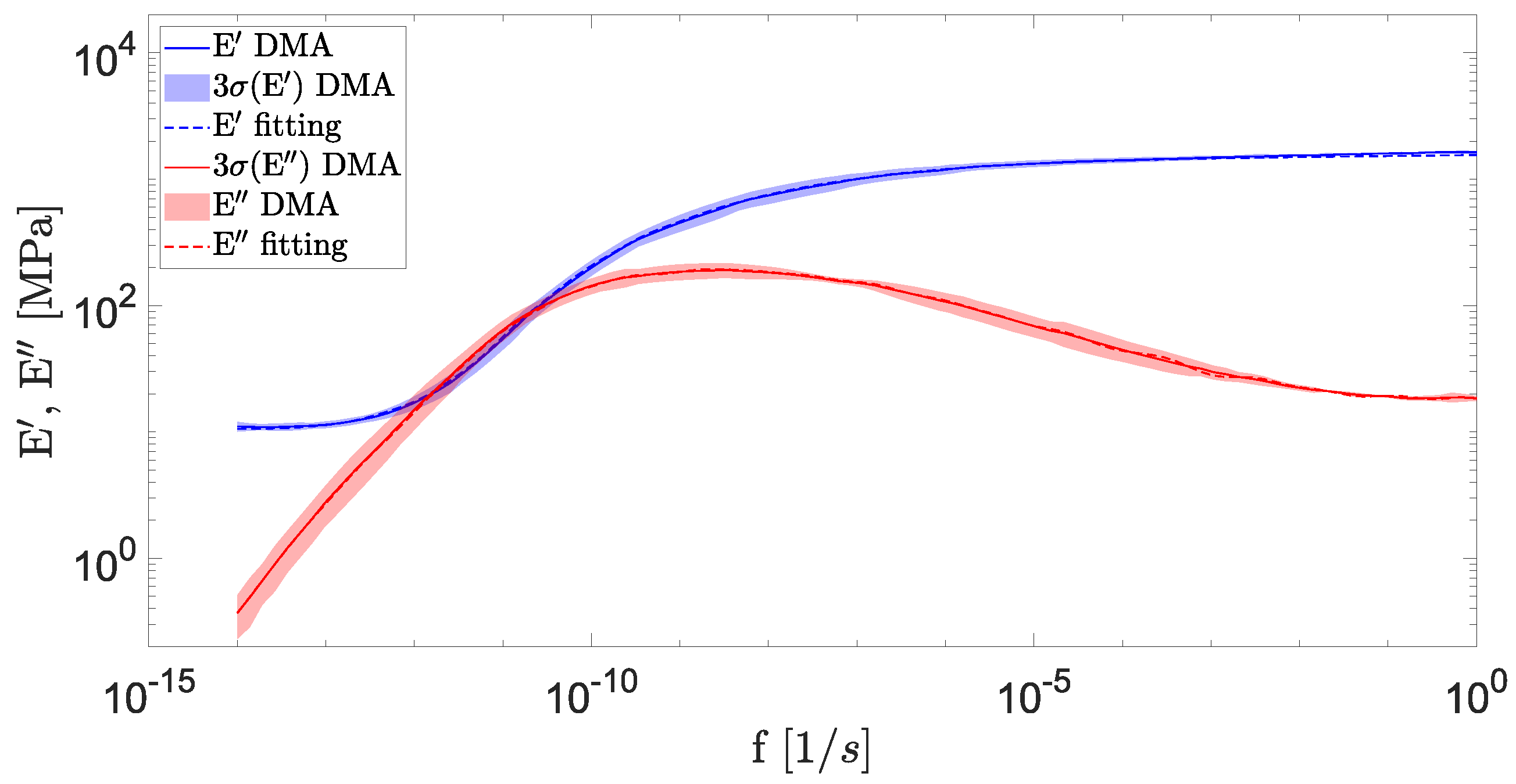
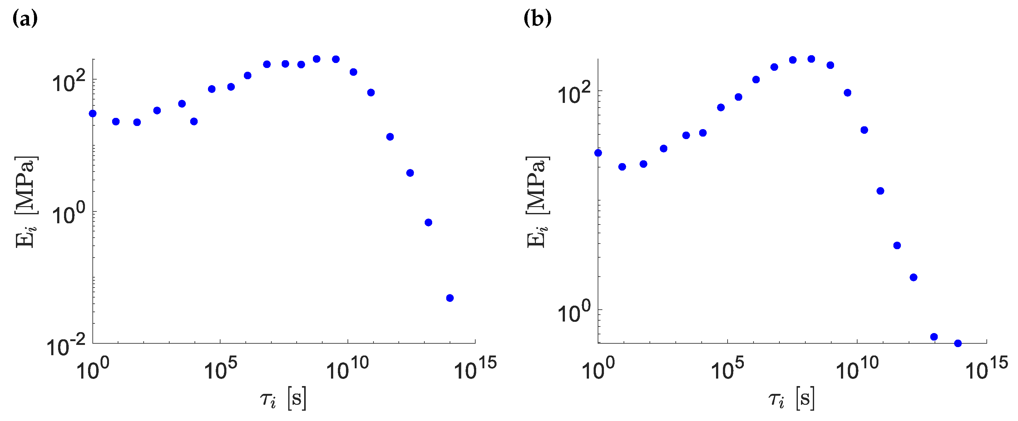
3.2. Fitting to Viscoelastic Model

For the viscoelastic resin, the relationship between the uniaxial varying strain, $ϵ\left(t\right)$, and the uniaxial varying stress, $\sigma \left(t\right)$, can be written through the relaxation modulus $E\left(t\right)$:

$$\sigma \left(t\right)={\int }_0^{t}E(t-s){\displaystyle \frac{dϵ\left(s\right)}{ds}}ds$$

(1)

The relaxation modulus could be represented through the Prony expansion series as:

$$E\left(t\right)=E_0-\sum _{i=1}^N{E}_i{e}^{-{\displaystyle \frac{t}{{\tau }_i}}}$$

(2)

where N is the number of relaxation modes, $E_0$ is the instantaneous modulus, $E_i$ are the Prony coefficients, and ${\tau }_i$ are the relaxation times.

In this work, the experimentally obtained master curves for $E^{\prime }$ and $E^{″}$ are fit to the Prony expansion series in Equation (2), which can be written in the frequency domain as:

$$E^{\prime }\left(\omega \right)=E_0-\sum _{i=1}^N{E}_i{\displaystyle \frac{{\left(\omega {\tau }_i\right)}^2}{1+{\left(\omega {\tau }_i\right)}^2}}$$

(3)

$$E^{″}\left(\omega \right)=\sum _{i=1}^N{E}_i{\displaystyle \frac{\omega {\tau }_i}{1+{\left(\omega {\tau }_i\right)}^2}}$$

(4)

To fit the experimental data to the Prony expansion series and evaluate the parameters in Equations (3) and (4), the approach detailed in [44] is used. According to [44], the instantaneous modulus $E_0$, the Prony coefficients $E_i$ and the relaxation time ${\tau }_i$ can be categorized into two sets. This categorization enables the fitting process to be divided into two separate optimization approaches, the linear least square solver (LLSS) and the particle swarm optimization (PSO), with each approach specifically targeting one of these sets. Specifically, $E_0$ and ${\tau }_i$ form the first set (SET-I). Bounds for the SET-I parameters can be can be pre-estimated (for $E_0$ data from the high-frequency domain can be used and for ${\tau }_i$ the interval can be approximated as the logarithmic scale of the test duration divided by N). The parameters $E_i$ form the second set (SET-II). The storage modulus and loss modulus are linearly related to SET-II parameters. Accordingly to this distinction in sets, the PSO method is suitable for selecting and optimizing SET-I, while the LLSS method can be used to determine SET-II directly once SET-I is known.

Throughout the whole optimization process, the relative error is taken as the objective function J,

$$J=\sum _{\omega }{\left({\displaystyle \frac{E_0}{E^{\prime }\left(\omega \right)}}-1-\sum _{i=1}^N{\displaystyle \frac{E_i}{E^{\prime }\left(\omega \right)}}{\displaystyle \frac{1}{1+{\left(\omega {\tau }_i\right)}^2}}\right)}^2+\sum _{\omega }{\left(1-{\displaystyle \frac{E_i}{E^{″}\left(\omega \right)}}{\displaystyle \frac{\omega {\tau }_i}{1+{\left(\omega {\tau }_i\right)}^2}}\right)}^2$$

(5)

To start the optimization, $E_0$ and ${\tau }_i$ of each particle are first designated with random values within the bounds as the initial guess by PSO algorithm. After that, LLSS is carried out to compute $E_i$ with the initial guess for $E_0$ and ${\tau }_i$. LLSS requires ${\displaystyle \frac{\partial J}{\partial G_i}}=0$ to reach the minimize, which leads to

$$E_i=B_{ij}^{-1}{A}_j$$

(6)

where

$$A_i=\sum _{\omega }\left(\left({\displaystyle \frac{E_0}{E^{\prime }\left(\omega \right)}}-1\right){\displaystyle \frac{1}{E^{\prime }\left(\omega \right)}}{\displaystyle \frac{1}{1+{\left(\omega {\tau }_i\right)}^2}}+{\displaystyle \frac{1}{E^{″}\left(\omega \right)}}{\displaystyle \frac{\omega {\tau }_i}{1+{\left(\omega {\tau }_i\right)}^2}}\right)$$

(7)

$$B_{ij}=\sum _{\omega }{\displaystyle \frac{\frac{1}{E^{\prime }{\left(\omega \right)}^2}+\frac{{\omega }^2{\tau }_i{\tau }_i}{E^{″}{\left(\omega \right)}^2}}{(1+{\left(\omega {\tau }_i\right)}^2)(1+{\left(\omega {\tau }_j\right)}^2)}}$$

(8)

Once $E_i$ are determined, J is computed and the next set of $E_0$ and ${\tau }_i$ are selected using the PSO algorithm based on its value. The above procedures are repeated until the convergence criterion is met.

In this work, to fit the experimental data to the Prony series expansion, the PSO is run with a total number of particles equal to $N_{PSO}=500$, a maximum number of iteration $N_{max}=2000$, a maximum wait $N_{wait}=2000$, and a convergence tolerance of ${10}^{-6}$.

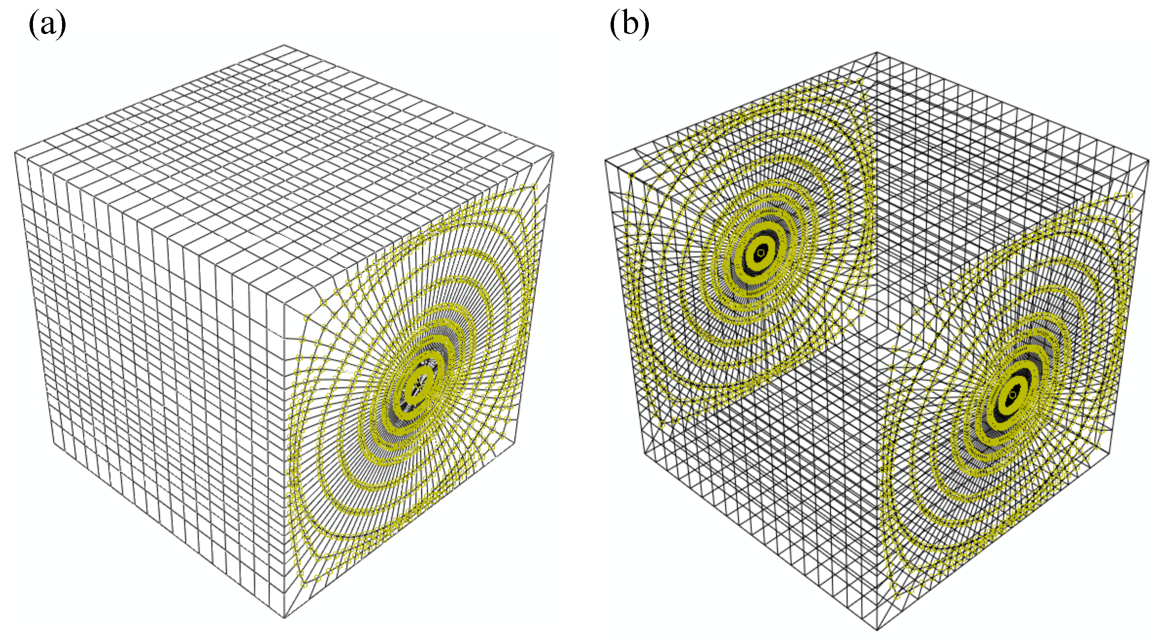
4. Composite Material Finite Element Modeling

To extend the insights gained from the epoxy resin system to the UD CFRP material, two FEM models are developed for its 3D RVE. Each model represents a fiber filament embedded within a unit cell cube of resin, as illustrated in Figure 4. In this setup, the x-axis is aligned with the fiber’s longitudinal direction, while the y- and z-axes are perpendicular to it. The diameter of the fiber filament is $d=7\mu$m, [51], and the cube side is $l=7.7\mu$m, so that the fiber volume fraction, $V_f$, is equal to $0.65$.

The fiber in each model is represented as a linear-elastic, transversely isotropic material, with mechanical properties specified in

Table 1. Torayca^® T300 elastic properties.

Properties	Value
Longitudinal Modulus [GPa]	233
Transverse Modulus [GPa]	23.1
Shear Modulus [GPa]	8.693
Longitudinal Poisson’s Ratio	0.2

for Torayca^® T300 fibers. The matrix is modeled as a linear-viscoelastic, isotropic material. The key difference between the models lies in the matrix properties: one uses values obtained experimentally before UV exposure, while the other uses values measured after UV exposure.

The viscous behavior of the UD CFRP can be modeled by extending the 1D stress relaxation equation, Equation (1), to a 3D case. This extension involves defining the relaxation matrix components, $C_{ij}$, to relate the stress and strain matrix components, ${\sigma }_{ij}$ and ${ϵ}_{ij}$, as follows:

$${\sigma }_{ij}\left(t\right)=\sum C_{ij}\left(t\right){ϵ}_{ij}\left(t\right)$$

(9)

Due to the distinct properties of the fiber and resin in the RVE, the strain and stress fields are nonuniform, requiring the transition from heterogeneous to homogenized fields via volume averaging,

$${\overline{\sigma }}_{ij}\left(t\right)={\displaystyle \frac{1}{V}}{\int }_V{\sigma }_{ij}(x,y,z)dV$$

(10)

$${\overline{ϵ}}_{ij}\left(t\right)={\displaystyle \frac{1}{V}}{\int }_V{ϵ}_{ij}(x,y,z)dV$$

(11)

Equation (9) can be rewritten using averaged stress tensor, ${\overline{\sigma }}_{ij}\left(t\right)$, and averaged strain tensors, ${\overline{ϵ}}_{ij}\left(t\right)$, as follows:

$${\overline{\sigma }}_{ij}=\sum C_{ij}\left(t\right){\overline{ϵ}}_{ij}\left(t\right)$$

(12)

Given the UD CFRP’s symmetry about its isotropy plane, Equation (12) becomes

$$\left[\begin{array}{c}{\overline{\sigma }}_{11}\left(t\right)\\ {\overline{\sigma }}_{22}\left(t\right)\\ {\overline{\sigma }}_{33}\left(t\right)\\ {\overline{\sigma }}_{12}\left(t\right)\\ {\overline{\sigma }}_{13}\left(t\right)\\ {\overline{\sigma }}_{23}\left(t\right)\end{array}\right]=\left[\begin{array}{cccccc}{C}_{11}\left(t\right)& C_{12}\left(t\right)& C_{13}\left(t\right)& 0& 0& 0\\ C_{12}\left(t\right)& C_{22}\left(t\right)& C_{23}\left(t\right)& 0& 0& 0\\ C_{13}\left(t\right)& C_{23}\left(t\right)& C_{33}\left(t\right)& 0& 0& 0\\ 0& 0& 0& C_{44}\left(t\right)& 0& 0\\ 0& 0& 0& 0& C_{55}\left(t\right)& 0\\ 0& 0& 0& 0& 0& C_{66}\left(t\right)\end{array}\right]\left[\begin{array}{c}{\overline{ϵ}}_{11}\left(t\right)\\ {\overline{ϵ}}_{22}\left(t\right)\\ {\overline{ϵ}}_{33}\left(t\right)\\ {\overline{ϵ}}_{12}\left(t\right)\\ {\overline{ϵ}}_{13}\left(t\right)\\ {\overline{ϵ}}_{23}\left(t\right)\end{array}\right]$$

(13)

To compute the relaxation matrix components in Equation (13), four analyses are needed in the numerical simulation. Each analysis consists of two quasi-static *VISCO steps. In the first step, all the averaged strains are set to zero, but one which is given a unit value (e.g., ${\overline{ϵ}}_{11}\left(t\right)=1,{\overline{ϵ}}_{22}\left(t\right)={\overline{ϵ}}_{33}\left(t\right)={\overline{ϵ}}_{12}\left(t\right)={\overline{ϵ}}_{13}\left(t\right)={\overline{ϵ}}_{23}\left(t\right)=0$). The time duration of the strain application is ${10}^{-2}$ s, so that the composite behaves elastically. In the second step the unit averaged strain is held constant over a much larger period to study the relaxation. Particularly, a period of ${10}^9$ is chosen for the second step, which corresponds to approximately 32 years.

To load the RVE according to the strain component in Equation (13), periodic boundary conditions (PBCs) are applied. The PBCs applied at the side faces are collected in Equations (14)–(16), where u, v, and w are the displacement along x, y, and z axis, respectively.

$$\begin{array}{c}\hfill u(l/2,y,z)-u(-l/2,y,z)={\overline{ϵ}}_{11}l\\ \hfill v(l/2,y,z)-v(-l/2,y,z)={\overline{ϵ}}_{12}l\\ \hfill w(l/2,y,z)-w(-l/2,y,z)={\overline{ϵ}}_{13}l\end{array}$$

(14)

$$\begin{array}{c}\hfill u(x,l/2,z)-u(x,-l/2,z)={\overline{ϵ}}_{21}l\\ \hfill v(x,l/2,z)-v(x,-l/2,z)={\overline{ϵ}}_{22}l\\ \hfill w(x,l/2,z)-w(x,-l/2,z)={\overline{ϵ}}_{23}l\end{array}$$

(15)

$$\begin{array}{c}\hfill u(x,y,l/2)-u(x,y,-l/2)={\overline{ϵ}}_{31}l\\ \hfill v(x,y,l/2)-v(x,y,-l/2)={\overline{ϵ}}_{32}l\\ \hfill w(x,y,l/2)-w(x,y,-l/2)={\overline{ϵ}}_{33}l\end{array}$$

(16)

The application of PBCs necessitates the inclusion of dummy nodes in the model, with each node assigned a nodal displacement corresponding to a specific averaged strain in Equations (14)–(16).

To easily apply PBCs, a Python code communicating with ABAQUS is developed, thus avoiding complex and time-consuming graphical user interface (GUI) input. The code developed finds nodes on faces and sorts all the nodes according to their coordinates. Then, the code matches the ones on opposite faces, and the PBCs are applied. A schematic representation of the PBC application is shown in Figure 5. To avoid redundant constraints on edges and vertices, laying either to two or three planes simultaneously, edges and vertices are excluded from faces, and vertices are also excluded from edges, as can be noted in Figure 5. Then, their PBC equations are given individually as a combination of the PBCs on the side faces. Opposite edges and opposites vertices are connected to have a correct coupling in any load case.

Given that the average strain is imposed to be unitary, the averaged stress components computed at the end of each analysis provide the effective relaxation matrix component.

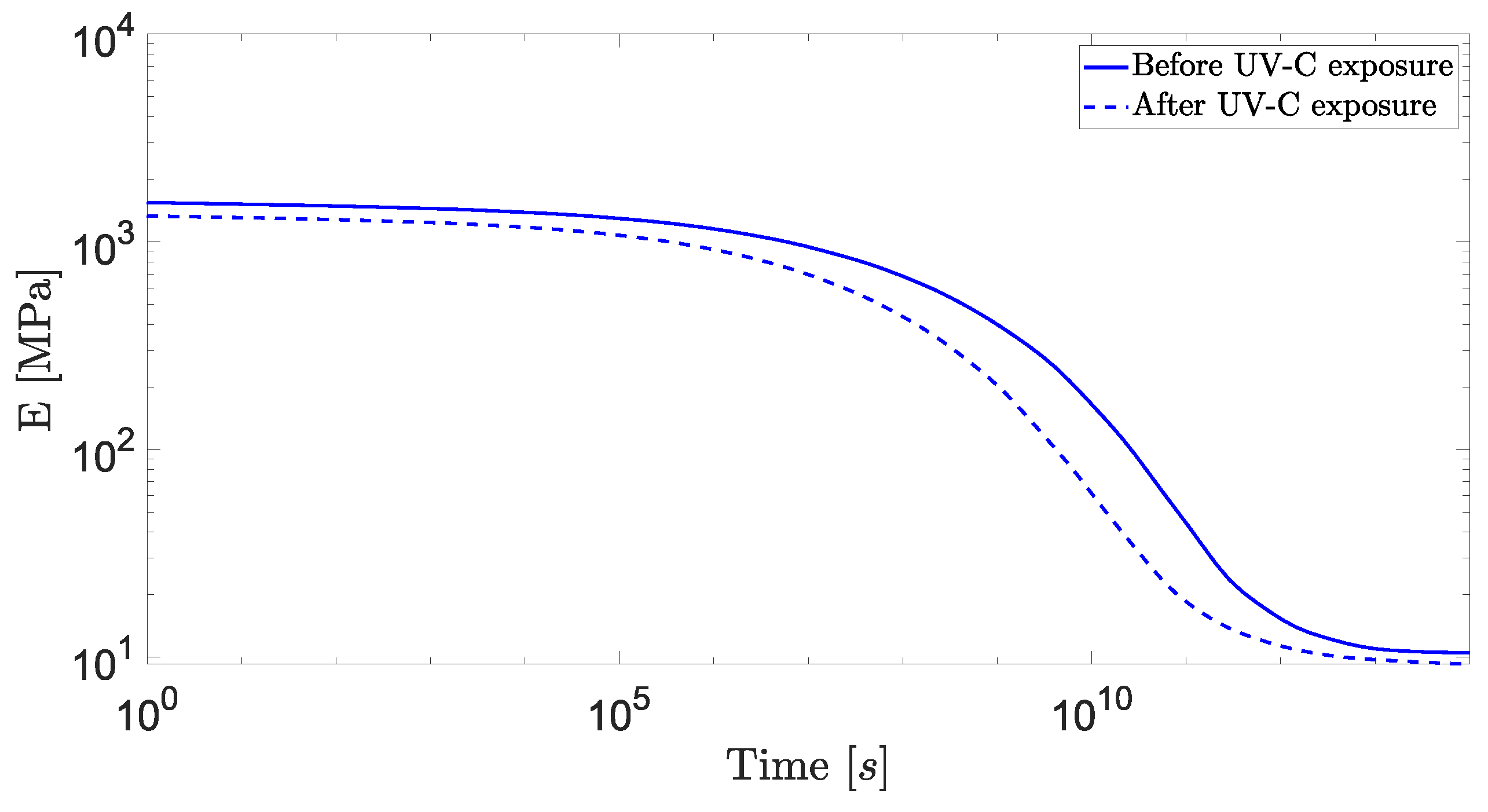
5. Matrix Experimental Characterization Results

This section presents and discusses the results of the experimental characterization of the matrix. First, the mastercurves and their fittings are shown. Following that, the relaxation modulus, obtained using the computed Prony series coefficients, are presented for both pre- and post-UV-C exposure, with comparisons provided.

The mastercurve obtained for the resin both before and after UV-C exposure, with respect to a reference temperature $T_{ref}$ = 40°, are collected in Figure 6 and Figure 7, along with their fittings. The blue and red solid lines represent the experimental data, obtained as the the averages of tests conducted on three distinct samples, for the storage modulus and loss modulus, respectively, while the dashed lines in the same colors indicate the corresponding fit results. The fitted curves align well with the experimental data.

The mastercurve obtained for the resin both before and after UV-C exposure, with respect to a reference temperature $T_{ref}$ = 40°, are shown in Figure 6 and Figure 7, along with their respective fittings. The blue and red solid lines represent the experimental data, obtained as the the averages of tests conducted on three distinct samples, for the storage modulus and loss modulus, respectively, with the shaded area indicating the $3\sigma$ region. The dashed lines in the same colors indicate the corresponding fit results. The fitted curves align well with the experimental data.

The storage modulus of the unexposed resin at a unit frequency is 1.63 GPa, while the storage modulus of the exposed resin is 1.45 GPa, indicating a 15% reduction in storage modulus after UVC exposure. This decrease aligns with literature findings on epoxy-based shape memory polymers (SMPs), where the storage modulus drops at the glassy stage following UV exposure, as reported in [56].

The corresponding Prony series parameters are collected in

Table 2. Coefficient of the Prony Series for CYCOM^® 823 RTM before and after UV-C exposure.

Index	Before UV-C Exposure		After UV-C Exposure
	${\mathit{E}}_{\mathit{i}}$  [MPa]	${\mathit{\tau }}_{\mathit{i}}$  [s]	${\mathit{E}}_{\mathit{i}}$  [MPa]	${\mathit{\tau }}_{\mathit{i}}$  [s]
0	1568.94	–	1352.82	–
1	30.33	1.00 $\times {10}^0$	27.03	1.00 $\times {10}^0$
2	22.91	8.11 $\times {10}^0$	20.16	8.49 $\times {10}^0$
3	22.31	5.48 $\times {10}^1$	21.40	5.62 $\times {10}^1$
4	33.64	3.34 $\times {10}^2$	29.62	3.38 $\times {10}^2$
5	42.64	3.16 $\times {10}^3$	39.10	2.50 $\times {10}^3$
6	22.97	9.31 $\times {10}^3$	41.19	1.10 $\times {10}^4$
7	71.15	4.66 $\times {10}^4$	70.36	5.49 $\times {10}^4$
8	76.83	2.64 $\times {10}^5$	87.60	2.62 $\times {10}^5$
9	113.97	1.18 $\times {10}^6$	126.42	1.25 $\times {10}^6$
10	168.69	6.73 $\times {10}^6$	164.57	6.30 $\times {10}^6$
11	171.35	3.56 $\times {10}^7$	191.08	3.26 $\times {10}^7$
12	167.29	1.49 $\times {10}^8$	195.25	1.70 $\times {10}^8$
13	203.33	5.95 $\times {10}^8$	171.21	9.24 $\times {10}^8$
14	201.21	3.39 $\times {10}^9$	95.89	4.25 $\times {10}^9$
15	128.81	1.66 $\times {10}^{10}$	43.79	1.88 $\times {10}^{10}$
16	63.00	8.06 $\times {10}^{10}$	12.14	7.86 $\times {10}^{10}$
17	13.47	4.53 $\times {10}^{11}$	3.85	3.46 $\times {10}^{11}$
18	3.81	2.76 $\times {10}^{12}$	1.97	1.50 $\times {10}^{12}$
19	0.68	1.45 $\times {10}^{13}$	0.56	9.25 $\times {10}^{12}$
20	0.05	1.00 $\times {10}^{14}$	0.49	7.72 $\times {10}^{13}$

. Additionally in Figure 8, the correlation between $G_i$ and ${\tau }_i$ is shown. It is evident that $G_i$ exhibits a general trend of higher values at lower ${\tau }_i$, with a consistent decrease as ${\tau }_i$ increases for the resin both before and after UV-C exposure. This behavior aligns with typical observations in viscoelastic spectra [57].

Once the Prony series coefficients are obtained, it is possible to provide a representation of the relaxation modulus in time according to Equation (2). The time-dependent relaxation modulus for the resin, both before and after UV-C exposure, is shown in Figure 9.

As shown in Figure 9, the instantaneous modulus of the resin decreases after UV-C exposure, dropping from $1568.94$ MPa to $1352.82$ MPa, which is the $86.22\%$ of the unexposed instantaneous value. Moreover, the degradation of the resin’s properties post-UV-C exposure occurs significantly faster than for the unexposed resin. After ${10}^9$ seconds, which corresponds to approximately 32 years, the relaxation modulus of the unexposed polymer is $399.89$ MPa, representing $25.49\%$ of the unexposed instantaneous value, while for the UV-C-exposed polymer, the relaxation modulus drops to $203.83$ MPa, or $15.07\%$ of the exposed instantaneous value. The modulus after ${10}^9$ seconds for the UV-C-exposed samples is approximately $50.98\%$ of the modulus value at ${10}^9$ seconds for the samples that were not exposed to UV-C.

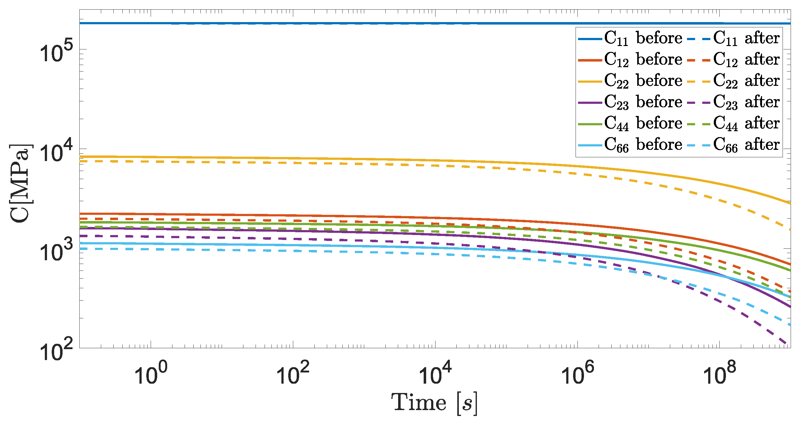
6. Composite Material Finite Element Modeling Results

This section presents and discusses the results of the FEM simulations for the composite material under investigation. It includes the results from two developed models: one incorporating the viscoelastic properties of the resin before UV-C exposure, which serves as a baseline for the long-term viscoelastic behavior of the composite, and another incorporating the viscoelastic properties of the resin after UV-C exposure, which quantifies the effects of UV-C exposure on the long-term viscoelastic behavior of the composite material. Figure 10 displays the relaxation matrix coefficients computed from the FEM simulations. Specifically, the coefficients $C_{11}$, $C_{12}$, $C_{13}$, $C_{21}$, $C_{22}$, $C_{23}$, $C_{44}$, and $C_{66}$ are shown. For the model incorporating the resin properties before UV-C exposure, these coefficients are represented by solid lines, while for the model incorporating the resin properties after UV-C exposure, they are represented by dashed lines.

From Figure 10, it can be observed that all the relaxation coefficients values at the initial time point are lower when the polymer’s properties after UV-C exposure are considered. This denotes that UV exposure results in a reduction in the mechanical improvement envisaged from the reinforcement, as already reported in [58]. The axial relaxation coefficient in the direction of the fiber’s longitudinal axis, $C_{11}$, has an initial value of $182.56$ GPa before UV-C exposure and only slightly reduces to $182.39$ GPa after UV-C exposure. The axial relaxation coefficient in the direction perpendicular to the fiber’s longitudinal axis, $C_{22}$, has an initial value of $8.35$ GPa before UV-C exposure that reduces to $7.52$ GPa after UV-C exposure. This reduction means that $C_{22}$ after UV-C exposure is $90.06\%$ of its pre-exposed value. The off-diagonal relaxation coefficients, $C_{12}$ and $C_{23}$, have initial values of 2.24 GPa and 1.60 GPa, respectively, before UV-C exposure, and 1.98 GPa and 1.33 GPa, after UV-C exposure. The values for $C_{12}$ and $C_{23}$ after UV-C exposure are $88.39\%$ and $83.13\%$ of their respective values before UV-C exposure. The shear stiffness coefficients, $C_{44}$ and $C_{66}$, have values of 1.83 GPa and 1.13 GPa, respectively, before UV-C exposure, and 1.64 GPa and 0.99 GPa, respectively, after UV-C exposure, which correspond to $89.62\%$ and $87.61\%$ of the initial $C_{44}$ and $C_{66}$ value before UV-C exposure. This decrement in performance at the initial time is attributed to the decrease in the instantaneous relaxation modulus of the polymer following UV-C exposure, as previously shown in Figure 9.

The performance degradation due to UV-C exposure increases over time, with the gaps between the coefficients obtained from the models including polymer’s properties before and after UV-C exposure widening. This trend is seen for all coefficients except $C_{11}$. After ${10}^9$ seconds, $C_{22}$ drops to 2.83 GPa before UV-C exposure and to 1.54 GPa after UV-C exposure. At this time, the $C_{22}$ value for UV-C-exposed CFRP is only 54.42% of the value it would have had without UV-C exposure. Similarly, $C_{12}$ and $C_{23}$ decrease to 0.69 GPa and 0.26 GPa, respectively, without exposure, while they fall to 0.37 GPa and 0.11 GPa if exposure is considered. After ${10}^9$ seconds, $C_{12}$ and $C_{23}$ after UV-C exposure are 53.62% and 42.31% of the corresponding values in the absence of UV-C exposure. Finally, the shear stiffness coefficients $C_{44}$ and $C_{66}$ decrease to 0.60 GPa and 0.32 GPa, respectively, before UV-exposure, and to 0.32 GPa and 0.17 GPa after UV-C exposure. After ${10}^9$ seconds, the exposed $C_{44}$ and $C_{66}$ coefficients are $53.33\%$ and $53.12\%$ of the corresponding values before UV-C exposure.

The time-dependent and radiation-sensitive behaviors of $C_{12}$, $C_{13}$, $C_{21}$, $C_{22}$, $C_{23}$, $C_{44}$, and $C_{66}$ arise from the significant influence of both the matrix and fiber phases on these coefficients. In this study, the observed reduction in these coefficients over time is attributed to the resin’s viscoelasticity, while the accelerated degradation after UV exposure is linked to the resin’s sensitivity to radiation, which accelerates the deterioration over time, as illustrated in Figure 9. Conversely, $C_{11}$ maintains a constant value over time both before and after UV-C exposure. This stability is due to the fiber’s time-independent and radiation-insensitive behavior of the fiber, which dominates the composite’s behavior along the direction aligned with the fiber’s longitudinal axis, resulting in an axial relaxation coefficient that mirrors the fiber’s properties.

The results presented in this investigation align with previous findings. Yan et al. studied the combined effects of ultraviolet (UV) radiation and water spraying on the mechanical properties of flax fabric/epoxy composites and observed a decline in both tensile and flexural properties after exposure. Specifically, after 1500 h of exposure, the tensile modulus decreased by 34.9%, while the flexural modulus was reduced by 10.2% [59]. Similarly, UV aging has been shown to deteriorate the mechanical properties of epoxy-based CFRP, with longitudinal compression strength decreasing by 23% [17]. DMA tests further confirmed reductions in the storage modulus for both glass fiber-reinforced shape memory polymer composites after UV exposure and for CFRP made from recycled fibers [18,58]. Conversely, some studies have reported improvements in the mechanical properties of PMCs following prolonged exposure [60,61]. Additionally, a comprehensive ten-year study examining the mechanical property changes in PMCs under worldwide outdoor exposure is available in the literature [62]. The findings indicate that, for certain mechanical properties in exposed specimens, most results fell within the baseline scatter range, and in some cases, strength values exceeded those observed in unexposed specimens.

7. Conclusions

This work investigates the viscoelastic properties of an epoxy resin before and after exposure to UV-C radiation, simulating one year in LEO. These properties, once fitted with a Prony series, are then used to model the relaxation behavior of a UD CFRP following UV-C exposure.

First, the viscoelastic resin properties are analyzed by constructing master curves using DMA short-duration tests and the TTSP. By comparing the master curves before and after UV-C exposure, it is possible to assess how UV-C exposure influences the resin’s performance and durability. Particularly, after UV-C exposure, the resin’s instantaneous modulus decreases by approximately $15\%$. Over a projected period of 32 years, the unexposed resin’s modulus is expected to degrade to about $25\%$ of its initial value, whereas the exposed resin’s modulus degrades to roughly $15\%$ of its original value. The master curves are fitted to a Prony series expansion using a combination of LLSS and PSO. This approach yields fitted curves that closely align with the experimental data, further demonstrating how a stochastic optimization algorithm like PSO broadens the LLSS search space and enhances the likelihood of finding a globally optimal solution.

Then, two FEM models of the RVE for a UD CFRP are developed: one incorporating the time-dependent properties of the resin before UV-C exposure and the other those after exposure. Relaxation analyses on the FEM models homogenize the UD CFRP and extend the effects of UV-C exposure from the polymer matrix to the composite material. Along the fiber’s longitudinal direction, the relaxation stiffness coefficient shows minimal change between pristine and UV-C-exposed states, with a slight reduction in instantaneous value but no time-dependent degradation. In other directions, the matrix’s time-dependent and radiation-sensitive behavior leads to a noticeable decrease in performance over time. The corresponding stiffness coefficients exhibit an instantaneous reduction of approximately 10% following UV-C exposure, and over time, this difference between pre- and post-exposure values diverges, reaching a reduction of nearly 55% after 32 years.

The findings presented herein highlight the critical impact of UV radiation exposure on the long-term behavior of polymer-based composite materials. They demonstrate that ignoring the effects of radiation could lead to an overestimation of their properties, and that this overestimation increases with longer mission durations. During the design phase, it is therefore crucial to account for both radiation exposure and mission duration to ensure material durability. This consideration is vital to guarantee that structures constructed from polymer-based composite materials maintain the necessary performance standards throughout their operational lifespan, in line with mission requirements.

Worth noting is that, in an LEO environment, radiation exposure and the passage of time act simultaneously as degradation factors. Therefore, the current study, which examines these factors sequentially rather than concurrently, provides a preliminary analysis of their effects. The degradation observed, even with this sequential approach, underscores the need for further investigation into this phenomenon.

References

1. Tribble, A.C. The Space Environment: Implications for Spacecraft Design-Revised and Expanded Edition; Princeton University Press: Princeton, NJ, USA, 2020. [Google Scholar]
2. Grossman, E.; Gouzman, I. Space environment effects on polymers in low earth orbit. Nucl. Instrum. Methods Phys. Res. Sect. B Beam Interact. Mater. Atoms 2003, 208, 48–57. [Google Scholar] [CrossRef]
3. Han, J.H.; Kim, C.G. Low earth orbit space environment simulation and its effects on graphite/epoxy composites. Compos. Struct. 2006, 72, 218–226. [Google Scholar] [CrossRef]
4. Deev, I.; Nikishin, E. Effect of long-term exposure in the space environment on the microstructure of fibre-reinforced polymers. Compos. Sci. Technol. 1997, 57, 1391–1401. [Google Scholar] [CrossRef]
5. Schwam, D.; Litt, M. Evaluation of atomic oxygen resistant coatings for space structures. Adv. Perform. Mater. 1996, 3, 153–169. [Google Scholar] [CrossRef]
6. Golub, M.A.; Cormia, R.D. ESCA study of poly (vinylidene fluoride), tetrafluoroethylene-ethylene copolymer and polyethylene exposed to atomic oxygen. Polymer 1989, 30, 1576–1581. [Google Scholar] [CrossRef]
7. Scialdone, J.J. Characterization of the outgassing of spacecraft materials. In Proceedings of the Shuttle Optical Environment, Washington, DC, USA, 23–24 April 1981; Volume 287, pp. 2–9. [Google Scholar]
8. Rånby, B. Photodegradation and photo-oxidation of synthetic polymers. J. Anal. Appl. Pyrolysis 1989, 15, 237–247. [Google Scholar] [CrossRef]
9. Mahmoud, W.; Elfiky, D.; Robaa, S.; Elnawawy, M.; Yousef, S. Effect of atomic oxygen on LEO CubeSat. Int. J. Aeronaut. Space Sci. 2021, 22, 726–733. [Google Scholar] [CrossRef]
10. Tan, Q.; Li, F.; Liu, L.; Chu, H.; Liu, Y.; Leng, J. Effects of atomic oxygen on epoxy-based shape memory polymer in low earth orbit. J. Intell. Mater. Syst. Struct. 2018, 29, 1081–1087. [Google Scholar] [CrossRef]
11. Tagawa, M.; Yokota, K. Atomic oxygen-induced polymer degradation phenomena in simulated LEO space environments: How do polymers react in a complicated space environment? Acta Astronaut. 2008, 62, 203–211. [Google Scholar] [CrossRef]
12. Shin, K.B.; Kim, C.G.; Hong, C.S.; Lee, H.H. Prediction of failure thermal cycles in graphite/epoxy composite materials under simulated low earth orbit environments. Compos. Part B Eng. 2000, 31, 223–235. [Google Scholar] [CrossRef]
13. Lu, T.; Solis-Ramos, E.; Yi, Y.; Kumosa, M. UV degradation model for polymers and polymer matrix composites. Polym. Degrad. Stab. 2018, 154, 203–210. [Google Scholar] [CrossRef]
14. Singh, B.; Sharma, N. Mechanistic implications of plastic degradation. Polym. Degrad. Stab. 2008, 93, 561–584. [Google Scholar] [CrossRef]
15. Larché, J.F.; Bussière, P.O.; Therias, S.; Gardette, J.L. Photooxidation of polymers: Relating material properties to chemical changes. Polym. Degrad. Stab. 2012, 97, 25–34. [Google Scholar] [CrossRef]
16. Ding, J.; Cheng, L. Experimental study on ultrasonic three-point bending fatigue of CFRP under ultraviolet radiation. Eng. Fract. Mech. 2021, 242, 107435. [Google Scholar] [CrossRef]
17. Shi, Z.; Zou, C.; Zhou, F.; Zhao, J. Analysis of the mechanical properties and damage mechanism of carbon fiber/epoxy composites under UV aging. Materials 2022, 15, 2919. [Google Scholar] [CrossRef] [PubMed]
18. Tortorici, D.; Toto, E.; Santonicola, M.G.; Laurenzi, S. Effects of UV-C exposure on composite materials made of recycled carbon fibers. Acta Astronaut. 2024, 220, 367–373. [Google Scholar] [CrossRef]
19. Moon, J.B.; Kim, M.G.; Kim, C.G.; Bhowmik, S. Improvement of tensile properties of CFRP composites under LEO space environment by applying MWNTs and thin-ply. Compos. Part A Appl. Sci. Manuf. 2011, 42, 694–701. [Google Scholar] [CrossRef]
20. Jang, J.H.; Hong, S.B.; Kim, J.G.; Goo, N.S.; Lee, H.; Yu, W.R. Long-term properties of carbon fiber-reinforced shape memory epoxy/polymer composites exposed to vacuum and ultraviolet radiation. Smart Mater. Struct. 2019, 28, 115013. [Google Scholar] [CrossRef]
21. Jang, J.H.; Hong, S.B.; Kim, J.G.; Goo, N.S.; Yu, W.R. Accelerated testing method for predicting long-term properties of carbon fiber-reinforced shape memory polymer composites in a low earth orbit environment. Polymers 2021, 13, 1628. [Google Scholar] [CrossRef]
22. Zarrelli, M.; Skordos, A.A.; Partridge, I.K. Thermomechanical analysis of a toughened thermosetting system. Mech. Compos. Mater. 2008, 44, 181–190. [Google Scholar] [CrossRef]
23. Lange, J.; Månson, J.A.E.; Hult, A. Build-up of structure and viscoelastic properties in epoxy and acrylate resins cured below their ultimate glass transition temperature. Polymer 1996, 37, 5859–5868. [Google Scholar] [CrossRef]
24. Müller-Pabel, M.; Agudo, J.A.R.; Gude, M. Measuring and understanding cure-dependent viscoelastic properties of epoxy resin: A review. Polym. Test. 2022, 114, 107701. [Google Scholar] [CrossRef]
25. Woo, E.; Seferis, J.; Schaffnit, R. Viscoelastic characterization of high performance epoxy matrix composites. Polym. Compos. 1991, 12, 273–280. [Google Scholar] [CrossRef]
26. Saseendran, S.; Wysocki, M.; Varna, J. Evolution of viscoelastic behaviour of a curing LY5052 epoxy resin in the rubbery state. Adv. Compos. Mater. 2017, 26, 553–567. [Google Scholar] [CrossRef]
27. Cost, T.L.; Becker, E.B. A multidata method of approximate Laplace transform inversion. Int. J. Numer. Methods Eng. 1970, 2, 207–219. [Google Scholar] [CrossRef]
28. Baumgaertel, M.; Winter, H. Determination of discrete relaxation and retardation time spectra from dynamic mechanical data. Rheol. Acta 1989, 28, 511–519. [Google Scholar] [CrossRef]
29. Davies, A.; Anderssen, R.S. Sampling localization in determining the relaxation spectrum. J. Non-Newton. Fluid Mech. 1997, 73, 163–179. [Google Scholar] [CrossRef]
30. Honerkamp, J.; Weese, J. Determination of the relaxation spectrum by a regularization method. Macromolecules 1989, 22, 4372–4377. [Google Scholar] [CrossRef]
31. Mustapha, S.S.; Phillips, T. A dynamic nonlinear regression method for the determination of the discrete relaxation spectrum. J. Phys. D Appl. Phys. 2000, 33, 1219. [Google Scholar] [CrossRef]
32. Jiang, B.; Kamerkar, P.; Keffer, D.J.; Edwards, B. Using multiple-mode models for fitting and predicting rheological properties of polymeric melts. J. Appl. Polym. Sci. 2006, 99, 405–423. [Google Scholar] [CrossRef]
33. Suchocki, C.; Pawlikowski, M.; Skalski, K.; Jasiński, C.; Morawiński, Ł. Determination of material parameters of quasi-linear viscoelastic rheological model for thermoplastics and resins. J. Theor. Appl. Mech. 2013, 51, 569–580. [Google Scholar]
34. Simhambhatla, M.; Leonov, A. The extended Padé-Laplace method for efficient discretization of linear viscoelastic spectra. Rheol. Acta 1993, 32, 589–600. [Google Scholar] [CrossRef]
35. Selivanov, M.F.; Chernoivan, Y.A. A combined approach of the Laplace transform and Pade approximation solving viscoelasticity problems. Int. J. Solids Struct. 2007, 44, 66–76. [Google Scholar] [CrossRef]
36. Rekik, A.; Brenner, R. Optimization of the collocation inversion method for the linear viscoelastic homogenization. Mech. Res. Commun. 2011, 38, 305–308. [Google Scholar] [CrossRef]
37. Emri, I.; Tschoegl, N. Determination of mechanical spectra from experimental responses. Int. J. Solids Struct. 1995, 32, 817–826. [Google Scholar] [CrossRef]
38. Bradshaw, R.D.; Brinson, L. A sign control method for fitting and interconverting material functions for linearly viscoelastic solids. Mech. Time-Depend. Mater. 1997, 1, 85–108. [Google Scholar] [CrossRef]
39. Carrot, C.; Verney, V. Determination of a discrete relaxation spectrum from dynamic experimental data using the Pade-Laplace method. Eur. Polym. J. 1996, 32, 69–77. [Google Scholar] [CrossRef]
40. Cho, K.S. A simple method for determination of discrete relaxation time spectrum. Macromol. Res. 2010, 18, 363–371. [Google Scholar] [CrossRef]
41. Fernanda, M.; Costa, P.; Ribeiro, C. Parameter estimation of viscoelastic materials: A test case with different optimization strategies. AIP Conf. Proc. Am. Inst. Phys. 2011, 1389, 771–774. [Google Scholar]
42. Gerlach, S.; Matzenmiller, A. Comparison of numerical methods for identification of viscoelastic line spectra from static test data. Int. J. Numer. Methods Eng. 2005, 63, 428–454. [Google Scholar] [CrossRef]
43. Costa, M.F.P.; Ribeiro, C. Generalized fractional Maxwell model: Parameter estimation of a viscoelastic material. AIP Conf. Proc. Am. Inst. Phys. 2012, 1479, 790–793. [Google Scholar]
44. Cui, Z.; Brinson, L.C. A combination optimisation method for the estimation of material parameters for viscoelastic solids. Int. J. Comput. Sci. Math. 2014, 5, 325–335. [Google Scholar] [CrossRef]
45. Sun, C.T.; Vaidya, R.S. Prediction of composite properties from a representative volume element. Compos. Sci. Technol. 1996, 56, 171–179. [Google Scholar] [CrossRef]
46. Huang, Y.; Jin, K.K.; Ha, S.K. Effects of fiber arrangement on mechanical behavior of unidirectional composites. J. Compos. Mater. 2008, 42, 1851–1871. [Google Scholar] [CrossRef]
47. Ye, F.; Wang, H. A simple Python code for computing effective properties of 2D and 3D representative volume element under periodic boundary conditions. arXiv 2017, arXiv:1703.03930. [Google Scholar]
48. Liu, X.; Tang, T.; Yu, W.; Pipes, R.B. Multiscale modeling of viscoelastic behaviors of textile composites. Int. J. Eng. Sci. 2018, 130, 175–186. [Google Scholar] [CrossRef]
49. Palmeri, F.; Lambertini, L.; Laurenzi, S. Numerical relaxation analysis of carbon fiber reinforced polymers. Macromol. Symp. 2024, 413, 2400038. [Google Scholar] [CrossRef]
50. An, N.; Jia, Q.; Jin, H.; Ma, X.; Zhou, J. Multiscale modeling of viscoelastic behavior of unidirectional composite laminates and deployable structures. Mater. Des. 2022, 219, 110754. [Google Scholar] [CrossRef]
51. Kwok, K.; Pellegrino, S. Micromechanics models for viscoelastic plain-weave composite tape springs. Aiaa J. 2017, 55, 309–321. [Google Scholar] [CrossRef]
52. Pathan, M.; Tagarielli, V.; Patsias, S. Numerical predictions of the anisotropic viscoelastic response of uni-directional fibre composites. Compos. Part A Appl. Sci. Manuf. 2017, 93, 18–32. [Google Scholar] [CrossRef]
53. Kemnitz, R.A.; Cobb, G.R.; Singh, A.K.; Hartsfield, C.R. Characterization of simulated low earth orbit space environment effects on acid-spun carbon nanotube yarns. Mater. Des. 2019, 184, 108178. [Google Scholar] [CrossRef]
54. Anderson, B.J.; Smith, R.E. Natural Orbital Environment Definition Guidelines for Use in Aerospace Vehicle Development; Technical Memorandum 4527; NASA Marshall Space Flight Center: Huntsville, AL, USA, 1994. [Google Scholar]
55. Ward, I.M.; Sweeney, J. Mechanical Properties of Solid Polymers; John Wiley & Sons: Hoboken, NJ, USA, 2012. [Google Scholar]
56. Wong, T.T.; Lau, K.T.; Tam, W.Y.; Leng, J.; Wang, W.; Li, W.; Wei, H. Degradation of nano-ZnO particles filled styrene-based and epoxy-based SMPs under UVA exposure. Compos. Struct. 2015, 132, 1056–1064. [Google Scholar] [CrossRef]
57. Brinson, H.F.; Brinson, L.C. Polymer engineering science and viscoelasticity. Introduction 2008, 99, 157. [Google Scholar]
58. Al Azzawi, W.; Epaarachchi, J.; Leng, J. Investigation of ultraviolet radiation effects on thermomechanical properties and shape memory behaviour of styrene-based shape memory polymers and its composite. Compos. Sci. Technol. 2018, 165, 266–273. [Google Scholar] [CrossRef]
59. Yan, L.; Chouw, N.; Jayaraman, K. Effect of UV and water spraying on the mechanical properties of flax fabric reinforced polymer composites used for civil engineering applications. Mater. Des. 2015, 71, 17–25. [Google Scholar] [CrossRef]
60. Tan, Q.; Li, F.; Liu, L.; Liu, Y.; Leng, J. Effects of vacuum thermal cycling, ultraviolet radiation and atomic oxygen on the mechanical properties of carbon fiber/epoxy shape memory polymer composite. Polym. Test. 2023, 118, 107915. [Google Scholar] [CrossRef]
61. Tan, Q.; Li, F.; Liu, L.; Liu, Y.; Yan, X.; Leng, J. Study of low earth orbit ultraviolet radiation and vacuum thermal cycling environment effects on epoxy-based shape memory polymer. J. Intell. Mater. Syst. Struct. 2019, 30, 2688–2696. [Google Scholar] [CrossRef]
62. Dexter, H.B. Long-Term Environmental Effects and Flight Service Evaluation of Composite Materials; NASA Langley Research Center: Hampton, VA, USA, 1987; Volume 89067. [Google Scholar]
Figure 1. Low-pressure UV lamp used for the UV-C irradiation process in laboratory.
Fibers 12 00110 g001
Figure 2. Schematic representation of the experimental setup illustrating the configuration and relevant dimensions involved in the UV-C irradiation process.
Fibers 12 00110 g002
Figure 3. DMA-1 in single cantilever configuration: front view.
Fibers 12 00110 g003
Figure 4. FEM model of the RVE of the UD CFRP.
Fibers 12 00110 g004
Figure 5. Schematic representation of the application of PBC: (a) the Python code finds nodes on faces and sorts by coordinates; (b) facing nodes on opposite side are matched.
Fibers 12 00110 g005
Figure 6. Experimental data in solid lines and fitting results in dashed lines for the storage modulus and loss modulus as a function of frequency before UV-C exposure.
Fibers 12 00110 g006
Figure 7. Experimental data in solid lines and fitting results in dashed lines for the storage modulus and loss modulus as a function of frequency after UV-C exposure.
Fibers 12 00110 g007
Figure 8. The correlation between E i and τ i : (a) before UVC exposure; (b) after UVC exposure.
Fibers 12 00110 g008
Figure 9. Relaxation modulus before and after UV-C exposure.
Fibers 12 00110 g009
Figure 10. Relaxation stiffness matrix coefficient as a functions of time before and after UV-C exposure.
Fibers 12 00110 g010