Abstract
Wood and its processing into particles are, combined, the largest cost factor in the production of particleboard, followed by the cost of adhesive. Thus, reducing their cost is a goal of process optimization. This study investigated whether possible savings could be identified and quantified by determining the particle surface using automated three-dimensional laser-scanning technology (3D Particleview, Fagus-Grecon). The focus was on saving adhesive by sieving out adhesive-consuming fines. It was shown that, currently, with the actual prices for wood (89 €/t), particle preparation (37 €/t), and adhesive (570 €/t), the resulting additional costs for particles are overcompensated by the savings for adhesive with high adhesive content (e.g., 19%). The assumption of uniform distribution of adhesive on the total surface of all particles was checked for correctness using digital reflected light microscopy (VHX-5000, Keyence). Since urea-formaldehyde (UF) adhesive commonly used in particleboard production can only be detected with increased effort, phenol-formaldehyde (PF) adhesive was applied for the tests. Ultraviolet microspectrophotometry (UMSP) was used to rule out excessive penetration of the adhesive into the wooden tissue of the particles. The examination of the distribution of the adhesive over the surface showed that smaller particle sizes tended to be more heavily coated with adhesive. This means that the calculated savings still underestimate the real-life potential or that potential savings exist even with lower adhesive prices or higher prices for wood.
1. Introduction
The ability to offer a product with which, on the one hand, the customer can realize their wishes at the lowest cost and, on the other hand, the difference between revenue and costs is at a maximum requires efficient production.
Based on information from Aßmann (2015) [1] on the cost structure for wood-based materials (obviously particleboard), the share of costs for prepared particles and adhesive is 68.9% of the total costs (Table 1). In material terms, particles and adhesive make up the entire material, excluding hardener and additives (e.g., wax). If an adhesive content of 9% (solid adhesive per dry wood) is assumed for the entire board, the mass-related share of the adhesive in the dry mass of the board is around 8%, and the remaining share (about 90%) is almost entirely accounted for by the wood. Details of common adhesive contents are given by Gfeller (as cited in [2] (p. 119)) (face layer: 10–12%, core layer: 6–8%) and Ressel (as cited in [3] (p. 26)) (face layer: 8–14%, core layer: 4–8%, entire board: 4–10%). Therefore, saving wood and adhesive is an important element for achieving economic goals.

Table 1.
Costs for the production of particleboard [1] and their proportions.
With a global production of 97.5 million m3 in 2019 [4], particleboard is one of the most economically significant wood-based materials in terms of production volume. In Europe, particleboard accounted for 54.2% (32.1 Mm3) of total wood-based panel production (59.2 Mm3) in 2019 (excluding Russia and Turkey), making it the most important wood-based panel in terms of product volume here as well. Moreover, 67% of the particleboard traded in Europe is purchased and processed by the furniture industry, 26% goes to the construction sector (incl. doors and flooring), 2% is used for packaging, and 5% is used in other applications [5] (pp. 36–37).
Since particleboard essentially consists of wood particles bonded together with adhesive, these two parameters determine the board properties when the density [6,7,8,9,10] and structure (e.g., particle orientation [11,12] and density profile [13]) of the boards are excluded. The interaction of the particles as a composite takes place via their overlapping surfaces, particularly the adhesive bond presented here, whereby these transfer the properties of the wood from which the particles are made to the resulting material [14] (p. 668). The effective overlap area is determined by the extent of compression of the wood over its natural density in the hot-pressing process [14] (pp. 815–816), [3] (p. 7) and the particle geometry, i.e., dimensions and shape. Dunky (2002) [14] (p. 668) explain that the effective overlap area can be increased by reducing the particle thickness for the same particle length and by lengthening the particle for the same particle thickness. Both cases effectively mean an increase in the slenderness ratio, since this is defined as the quotient of length and thickness. Since the particles undergo an undesirable and sometimes considerable breakup during adhesive application [14] (p. 667), the final particle geometry, which is relevant to the overlapping surfaces and board properties, can thus stringently be determined first on adhesivized particles or after particle mat formatting, as was obviously already considered in an initial description of the current laser technology [15] used here.
Under otherwise unchanged conditions, an increase in adhesive content leads to an increase in board properties [14] (pp. 786–789), [16]. This is obvious because more adhesive is available at the contact surfaces between the particles. In other words, the amount of adhesive on the particle surface is increased. The same happens when the particle size is increased with unchanged adhesive content. Due to the shape-specific non-linear relationship between surface area and volume of geometric bodies [17] (pp. 79–80), an increase in particle size leads to a decrease in the total surface area of a particle sample of equal mass and thus to an increase in the surface-specific adhesive amount and, further, to increasing board properties. This can be seen in the results of experiments conducted by Benthien and Ohlmeyer (2016) [18] (pp. 24–25) and Istek et al. (2018) [19], which showed that the use of a coarse particle material for board manufacture leads to higher bending modulus of elasticity and bending strength. One study [18] found this to be the case for three-layered boards made with face layer particles of different manufacturers; another study [19] found this to be the case when using different sieve fractions in the layers. An argument that this is not a direct effect of the particle size on the board properties but of the amount of adhesive on the surface is suggested by the results of Kitahara and Kasagi (1955) [20]. They produced boards from particles of the same shape but proportionally different size with a constant surface-specific adhesive amount and found a reduction in the bending properties with increasing particle size.
Conversely, it follows from the increase in the surface-specific adhesive amount with increasing particle size that the surface-specific adhesive amount decreases with decreasing particle size. This is supported by sources [14] (p. 772), [21] (pp. 35–36) that speak of an “adhesive-consuming effect of the fine particles”. The authors of both sources mention the underapplication of adhesive to the larger particles as a result of the excessive binding of adhesive by the small particles. In practical terms, underapplication of adhesive is to be expected when, during the process, there is wear of the knives in the flaker, resulting in an increase in the fines content [22] and a further increase in the total particle surface.
While, to date, the technology has been lacking to determine changes in particle size composition, particularly the surface per gram of particle material, and to adjust the adhesive amount based on this information, this is possible with the recently developed 3D Particleview (Fagus-GreCon Greten GmbH & Co. KG, Alfeld, Germany) [15]. However, it is important to understand that only the dimensions (length, width, and thickness), the particle volume, and the particle surface are determined. If the mass of the measured particle sample is known as well, an additional statement can be made about the surface area per gram of particle material. A direct indication of the surface-specific adhesive amount is not obtained, but must be calculated assuming an even adhesive distribution over the total surface of all particles. However, it is not clear whether the adhesive can be assumed to be evenly distributed with respect to the particle surface over the particle sizes.
In this context, Dunky (1988, 1998) [23,24] and Pichelin and Dunky (2003) [25] cited a study by Meinecke and Klauditz (1962) [26] on the fact that the adhesive application of particles does not take place uniformly with a certain area-specific adhesive application, but, with reference to Wilson and Hill (1978) [27] as well as Eusebio and Generalla (1983) [28], with a certain preference for coarse particles. Dunky (2002) [14] (pp. 769–780) re-cite this state of knowledge and discuss aspects of adhesive distribution (droplet size, adhesive film on the particle surface) on the individual particles. Medved and Grudnik (2021) [29] list works by Ducan (1974) [30], Meinecke and Klauditz (1962) [26], and Dunky (1988) [23] with regard to the view that more adhesive accumulates on the surface of larger particles. Hill and Wilson (1978) [27] were used as a source for the suggestion that smaller particles receive more adhesive than larger particles. Medved and Grudnik (2021) [29] found that an increase in particle size results in an increase in the surface covered with adhesive when investigating particles adhesivized with fluorescent dyed urea-formaldehyde (UF) adhesive using a microscope with a fluorescent light source.
Zhu et al. (2011) [31] and Altgen et al. (2019) [32] used confocal laser scanning microscopy (CLSM) to analyze labeled particles. Altgen et al. were even able to quantify the distribution of UF adhesive in particleboard cross-sections by automatic image analysis. Although particleboard is predominantly manufactured with UF adhesive, phenol-formaldehyde (PF) adhesive was used in this study to determine the adhesive distribution, as it is already clearly visible to the naked eye without staining. Brady and Kamke (1988) [33] used this beneficial property to measure the penetration of PF adhesive into wood. The manual procedure used at the time can now be followed much faster and more accurately using digital image processing and analysis. For example, the digital reflected light microscope (Keyence VHX-5000, Keyence Corporation, Osaka, Japan) can produce depth-sharp images of three-dimensional samples. Three- and two-dimensional images are generated from different focal planes. An automatic area measurement allows a very accurate determination of the adhesive on the particle surface. To evaluate a successful wood modification, Biziks et al. (2020) [34] detected the penetration of low molecular PF resin into the cell wall using ultraviolet microspectrophotometry (UMSP). It is also an established method for the detection of naturally occurring phenolic components/extractives in wood tissue [35,36,37]. On the other hand, the method is thus very well suited to exclude the seepage of adhesive into the deeper wood tissue of the particles or even into the cell wall.
The first aim of this study was to show that, by means of particle measurement, in particular the determination of the particle surface and, based on this, the calculation of the surface-specific adhesive amount, potential savings in the particleboard process can be worked out and quantified. The second aim of the study was to determine the distribution of the adhesive over the particle size in order to prove the correctness of the assumed uniformity or to show that this assumption underestimates rather than overestimates the possible savings.
The experiments showed that there tends to be more adhesive on the surface of small particles than would be expected under the assumption of a uniform surface-specific adhesive amount over the entire particle material. Based on the results of the particle measurement, it was shown with a calculation example that possible savings in adhesive by excluding the adhesive-consuming fine fraction more than compensate financially for the resulting additional expenditure for wood with high adhesive content (e.g., 19%).
2. Materials and Methods
2.1. Wood Particles and Adhesive
The wood particles used were supplied by the particleboard manufacturer Swiss Krono sp z o.o. (Zary, Poland) and taken from the material flow for the core layer after screening. According to the manufacturer, the wood particles consist mainly of softwood (Scots Pine (Pinus sylvestris)).
Liquid PF adhesive (Prefere 14J466) with a solid content of 47% was obtained from Dynea Erkner GmbH (Erkner, Germany). Ammonium nitrate (NH4NO3) solution with 40% solid content was used as hardener.
2.2. Test Material Preparation
The wood particles supplied were used either as delivered or with adhesive applied to them. If adhesive was applied, this was performed in a rotary drum blender of 400 mm length and 310 mm diameter, equipped with an air-atomizing spray system (Düsen-Schlick GmbH, Untersiemau/Coburg, Germany). Before application, 3% hardener (hardener solid per adhesive solid) was added to the adhesive. With regard to the moisture content of the wood particles, water was added to the adhesive emulsion so that the adhesivized particles had a moisture content of 8%. For the adhesive application, the speed of the drum blender was set to 100 rpm while the adhesive was injected through a 1.8 mm nozzle under a pressure of about 2 bar. The adhesive injection was carried out at a 90° angle to the rotation axis. After application, the adhesive was cured in an oven (Heraeus Holding GmbH, Hanau, Germany) for 60 min at 103 °C. The selected adhesive contents (AC) (adhesive solid per dry wood) were 8% and 19%. The untreated wood particles were named Particle Material 1 (PM 1), and the adhesivized wood particles were named PM 2 (AC 8%) or PM 3 (AC 19%). For a visual impression of the particle materials, see Figure 1.
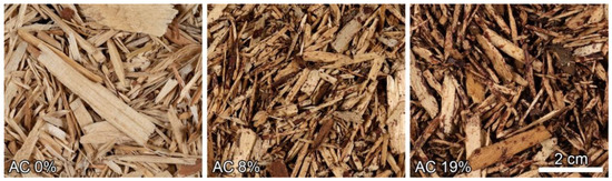
Figure 1.
Particle materials (PM) of different adhesive content (AC): PM 1 (AC 0%), PM 2 (AC 8%), PM 3 (AC 19%).
The particle materials were separated into fractions using a screening machine (AS 400 Control, Retsch GmbH, Haan, Germany) and sieves (200 mm diameter) with mesh sizes of 0.8, 1, 1.6, 2, 3.15, 4, 5, 8, 11.2, and 16 mm. Sieving time was 5 min with a rotation speed of 240 rpm. Approximately 50 g of particles were sieved per particle material.
An overview of particle material, adhesive content, and sieve mesh sizes (test material preparation design) can be seen in Table 1. A visual impression of the fractions can be seen in Figure 2. Before sieving and further investigations, the particle materials were air-conditioned at 20 °C and 65% relative humidity.
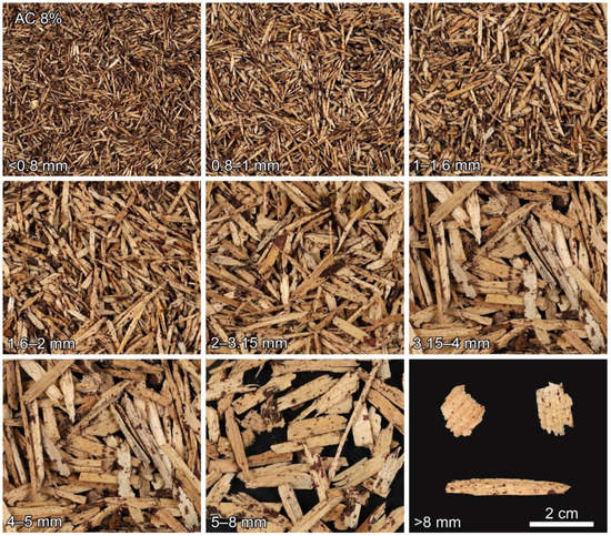
Figure 2.
Sieve-fractionated Particle Material 2 (AC 8%).
2.3. Particle Size Characterization Based on Sieve Analysis
Particle material characterization was carried out on the basis of the mass of particles remaining on a sieve (sieve residue) or, more precisely, their share of the total mass (relative mass). The procedure for sieving was the same as already described in Section 2.2, while three sieve runs were carried out for each particle material. The sieve analysis was based on the DIN 66165-1:2016-08, DIN 66165-2:2016-08, and DIN ISO 9276-1:2004-09 standards.
For the three sieving runs per particle material, the mean value, standard deviation and coefficient of variance were calculated. On the basis of the three sieving runs per particle material, any differences in the size (distribution) of the particle material were statistically investigated. This was achieved by applying the analysis tool JMP 16 from SAS Institute (Cary, NC, USA). The selection of the suitable test methods was carried out according to the scheme shown graphically in source [38]. This means that the data to be examined at first were tested for a normal distribution using the Shapiro–Wilk test at a significance level of α = 0.01. Since a normal distribution was present, it was tested for homogeneity of variance applying Levene’s test at a significance level of α = 0.05. Since homogeneity of variance was present, and the random sample size was larger than two (k = 3), it was tested for any statistically significant differences using the F test (the form to be applied for the analysis of variance (ANOVA)) at a significance level of α = 0.05. Since the number of data sets was greater than two, a post hoc analysis was carried out at a significance level of α = 0.05 to determine which data sets differed from each other. Since the data sets were balanced, Tukey’s test was used following the F test. The results of the post hoc analysis were given in the form of homogeneous groups (HG), indicating statistical distinctiveness by different letters.
2.4. Determination of Particle Surface Area (and Volume)
For the determination of the particle surface area, a 3D Particleview from Fagus-GreCon was used. The resolution of the measuring device is 0.1 mm in length and width and 0.02 mm in thickness. The chosen measurement mask was “min. area 1 mm2”, the conveyer belt speed was set to 15 m/min, and the speed of the first vibratory feeder was 16% and that of the second vibratory feeder was 45%. Since the software version 0.1.3.1 was used, the parameter “surface” was multiplied by a factor of two to obtain the particle surface area, i.e., the surface of the entire particle and not just its projection surface.
For further calculations, in particular for PM 1 (AC 0%), although the adhesivized particles were also measured, the total surface area was calculated for each sieve fraction obtained from the material preparation. In the first step, this was carried out separately for each run, but subsequently for the total of all runs. Moreover, the total of all runs and fractions was calculated and used for further calculations.
For a supplementary consideration, the parameter “volume” was employed.
2.5. Calculation of Surface-Specific Adhesive Amount
The surface-specific adhesive amount (SSAA) was calculated on the basis of the dry particle mass (Equation (1)) investigated (considering the moisture content (MC) of PM 1 of 11.1%),
the adhesive content, 8% or 19%, and the surface area per gram (dry particles), following Equation (2),
while the surface area per gram was calculated as the quotient of surface area and dry particle mass.
145.8 g × (1 − 11.1%) = 131.2 g,
SSAA = (dry wood mass × AC)/surface area per gram,
2.6. Adhesive Content (per Sieve Fraction)
The adhesive content (per sieve fraction) was calculated on the basis of the surface-specific adhesive amount of the particle material in total, the surface area (per fraction), and the dry particle mass (per fraction), following Equation (3):
AC = ((SSAA × surface area)/dry particle mass)/100.
2.7. Topochemical Detection of Phenolic Adhesive in Wooden Tissue by Using UMSP Technique
Particles taken randomly from the sieve fraction 3.15–4 mm of particle material PM1 (AC 0%), PM 2 (AC 8%), and PM 3 (AC 19%) were directly embedded under mild vacuum conditions in Spurr’s epoxy resin [39] as described by Kleist and Schmitt (1999) [40]. For optimal polymerization of the resin, the specimens were cured at 70 °C for 12 h. The cross-sectional areas of the particles were exposed by trimming with a razor blade. With an ultra-microtome, equipped with a diamond knife, semi-thin sections (1 µm) were prepared, transferred onto a microscopic quartz slide and thermally fixed. A drop of non-ultraviolet-absorbing glycerin was used to cover the sections under a quartz cover slip. These sections were also used for light microscopic examinations in order to have an overview of the entire cross-sectional area of the particles. This allowed the localization of regions infiltrated with adhesive.
Area scans and point measurements were carried out using an ultraviolet (UV) microspectrophotometer (UMSP 80, Carl Zeiss AG, Oberkochen, Germany). The microscope is equipped with a scanning stage. The integrated scanning program APAMOS® (Automatic-Photometric-Analysis of Microscopic Objects by Scanning, (Zeiss)) allows one to image certain areas of the sections at a constant wavelength. The coniferous (softwood) lignin shows the highest UV absorption at a wavelength of 280 nm. The phenolic adhesive also exhibits high absorption here.
The scanning fields have a local geometric resolution of 0.25 µm2 and a photometric resolution of 4096 grayscale levels. To visualize the absorbed intensity, the scale levels were converted into 14 basic colors. In addition, point measurements with a spot size of 1 µm2 were performed in the cell corners (CC), the compound middle lamella (CML), the secondary cell wall (S2), and for the adhesivized particles in the areas of the highly absorbent adhesive attachment in the cell lumen (AdCL). These measurements were taken in the range between 240 and 540 nm (pictured 248 nm and 450 nm).
2.8. Visual Detection of Phenolic Adhesive on Particle Surface Using Digital Reflected Light Microscopy
For particle material PM 2 (AC 8%) and PM 3 (AC 19%), the aim was to randomly take ten particles per sieve fraction. This was quite possible for the first eight sieve fractions, while for the sieve fraction > 8 mm, only two particles were available in the case of PM 2, and only one in the case of PM 3. As a reference, five particles were randomly taken from the sieve fraction 3.15–4 mm of particle material PM 1 (AC 0%) for examination. This resulted in a total number of 168 analyzed particles.
The particles taken in this way were examined individually under a digital reflected light microscope, a Keyence VHX-5000. This microscope is equipped with a powerful image-processing program with an integrated measuring tool that allows the surface structure of the particles to be evaluated both qualitatively and quantitatively. The uneven particle surfaces are first digitally scanned with a standard lens (VH-Z 20R, Keyence) at 150× magnification. In this way, three-dimensional images of the particles can be obtained. In the following, two-dimensional images are created to record the surface adhesive coating. The outlines of the individual particles are precisely outlined with a polygon tool and thus defined for the automatic detection of the visually well-distinct adhesive areas. In the figures shown in the results, the adhesive areas on the individual particles are highlighted in red. The total of these areas in relation to the total surface area of the particles then resulted in a degree of surface coverage (SC). The image files were taken with a resolution of 4800 × 3600 pixels; the pixel pitch is 1 µm with the above settings. The additionally created comma-separated values (CSV) files of the surface measurement were further analyzed in Microsoft Excel 2019 (Microsoft Corporation, Redmond, DC, USA). The SC of 168 particles was examined. In order to present the method as transparently as possible, all SC was depicted without consideration of the high variance. To show a clear tendency graphically, a trend line was calculated over the mean values of the SC of all the individual fractions.
2.9. Calculation of Possible Savings through the Selective Use of Sieve Fractions for Particleboard Production
For the calculation of the surface-specific adhesive amount and the adhesive content of a selection of sieve fractions, Equations (2) and (3) were used, while only considering the relevant sums of the particle mass and surface area.
The calculations of possible savings were made assuming a particleboard with a density of 650 kg/m3 (MC 10%), which means a dry mass of 591 kg per cubic meter of particleboard and a hardener content of 5.8% (solid per solid adhesive). For the calculations needed, the particle mass in the board was calculated following Equation (4). The relevant adhesive contents (e.g., 8%, 7.5%, 7.3%, …) were calculated as already mentioned following Equation (4).
Particle mass in board = 591 kg/m3/(1 + AC + (5.8% × AC))
In order to obtain the wood mass needed, from which only a part is then used for board production, factor f has to be calculated by which the particle mass in the board is to be increased. This factor is calculated as the quotient of the sum of the mass of all sieve fractions ∑m and the sum of the mass of the sieve fractions considered ∑mi following Equation (5).
f = ∑m/∑mi
The possible savings or, in case of particles, additional expense through the use of selected sieve fractions is calculated as follows:
- (a)
- The difference between the initial quantity of particles and the quantity of particles considered (particle mass in board) in the case of particles;
- (b)
- The product of the particle mass in board and the relevant adhesive content in the case of adhesive.
By multiplying the quantity and price, the additional cost or saving is obtained.
2.10. Calculation of Prices Based on Data from Aßmann (2015)
For the calculation of prices for particles and adhesive based on data from Aßmann (2015) [1], the following were assumed:
- Board density: 650 kg/m3 (MC 10%);
- Face-to-core layer ratio: 35/65;
- Face layer adhesive (hardener) content: 11% (2%);
- Core layer adhesive (hardener) content: 8% (6%);
- Adhesive solid content: 66%.
For the assumptions made, the particle mass per cubic meter of board was calculated for the face and core layer using Equation (4), as well as the adhesive mass based on the respective particle mass. After forming the sums, the costs for particles, particle preparation, and adhesive per cubic meter of board given by source [1] were divided by the respective sum to obtain the prices per kilogram. The price per kilogram of adhesive solids multiplied by the solids content gives the price per kilogram of adhesive emulsion.
3. Results
3.1. Particle Size Characterization (Sieve Analysis)
The data sets obtained from sieve analysis (see Supplementary Materials, Excel file) were normally distributed (Shapiro–Wilk test). The Levene’s test showed the presence of variance homogeneity across the particle materials (PM 1 (AC 0%), PM 2 (AC 8%), PM 3 (AC 19%)) for each of the fractions (<0.8 mm … 8–16 mm). Consequently, the F test was applied to test for any significant differences between the particle materials. Due to equal sample size, the Tukey’s test was used for subsequent post hoc analysis. The results (relative mass fraction, their fluctuation range (standard deviation and coefficient of variation), and the statistical mean value comparison (homogeneous groups)) of sieve-analyzing the particles of different adhesive contents are shown in Table 2.
Table 2.
Relative mass, fluctuation range (round brackets: standard deviation; square brackets: coefficient of variation), and results of statistical analysis (homogeneous groups, indicated as capital letters) of sieve-analyzing the particle materials of different adhesive contents.
Based on the statistical comparison of the relative mass fraction across the particle materials, it can be concluded that there are only minor differences between the particle material with an adhesive content of 0% and 8%, while the particle material with an adhesive content of 19% differs in most cases from the two others.
It should be noted here that the size reduction mentioned with reference to source [14] in the Introduction can be seen in the data set listed in Table 2. With an increase in the adhesive content from 8% to 19% and the associated increase in the duration of the adhesive application, a reduction in particle size in the smaller sieve fractions and an increase in particle size in the coarser sieve fractions can be observed. Although this initially seems inconsistent, it confirms the aforementioned correlation. Finally, it is to be expected that the resulting adhesivized fine particles agglomerate and do not appear as fine particles in the results of the sieve analysis.
3.2. Particle Surface Area (3D Particleview) and Surface Area per Gram Dry Particles
Table 3 lists the dry weights of Particle Material 1 (moist weight × (1 − 11.1%)) investigated with 3D Particleview measurements as the total of the three replicate measurements, the total of the determined particle surface areas, and the surface area per gram dry particles. For the raw data, see Supplementary Materials, Excel file.
Table 3.
Total dry particle mass and surface area of the three measurement runs as well as the calculated or extrapolatively corrected surface area per gram dry particles for each sieve fraction.
Figure 3 shows that the calculated surface area per gram dry wood (relative surface area) has to be incorrect for the fines sieve fraction. Contrary to what is logically expected, the relative surface area does not increase further with decreasing particle size. The reason for this was assumed to be an insufficient resolution of the measuring system in this size area and the relative surface was extrapolatively (assuming a linear relationship so as not to overestimate in any case; cautiously conservative approach) corrected on the relative surface of the two other sieve fractions:
y = −10,457x + 24,608 ↔ y = −10,457 × (0.8/2) + 24,608 ↔ 20,425 = −10,457 × 0.4 + 24,608

Figure 3.
Visualization of the relative, related to one gram of dry wood particles, surface area.
Another indicator that the measurement of the particles of the first fraction (<0.8 mm) is not reliable is that the volume per gram of particle material, and even more obviously its reciprocal value (g/cm3 or kg/m3), i.e., the density of the wood as a quotient of the initial weight and particle volume, is clearly different for this fraction compared to the other fractions:
- <0.8 mm; 1.52 cm3/g; 659 kg/m3;
- 0.8–1 mm; 2.48 cm3/g; 403 kg/m3;
- 1–1.6 mm; 2.79 cm3/g; 358 kg/m3;
- 1.6–2 mm; 2.87 cm3/g; 348 kg/m3;
- 2–3.15 mm; 2.92 cm3/g; 342 kg/m3;
- 3.15–4 mm; 2.99 cm3/g; 334 kg/m3;
- 4–5 mm; 3.01 cm3/g; 333 kg/m3;
- 5–8 mm; 2.97 cm3/g; 337 kg/m3;
- 8–16 mm; 3.07 cm3/g; 326 kg/m3.
Simply expressed, one could say that the determined volume is too low for the measured particle mass.
Based on the applied approach to solve the present inadequacy of the measurement system, the corrected data listed in Table 3 are used in the following.
The following list shows that the data of the replicate measurements, with the exception of the fraction > 8 mm (very low number of particles per measurement), are subject to little variation (given here: sieve fraction; mean value of surface area per gram of sample mass (n = 3); coefficient of variance):
- <0.8 mm; 12,243 mm2; ±7.0%;
- 0.8–1 mm; 15,420 mm2; ±2.5%;
- 1–1.6 mm; 11,168 mm2; ±2.6%;
- 1.6–2 mm; 8185 mm2; ±4.4%;
- 2–3.15 mm; 6324 mm2; ±2.3%;
- 3.15–4 mm; 5208 mm2; ±3.3%;
- 4–5 mm; 4776 mm2; ±3.4%;
- 5–8 mm; 4217 mm2; ±3.6%;
- 8–16 mm; 3963 mm2; ±38.6%.
3.3. Theoretical Surface-Specific Adhesive Amount
Based on the data given in Table 3 (weighting and surface area per gram dry wood) and the respective adhesive content considered (8%, 19%), the surface-specific adhesive amount is calculated as 10.3 g/m² and 24.4 g/m².
- AC 8%: (131.2 g × 8%)/1.02 m2 = 10.3 g/m2
- AC 19%: (131.2 g × 19%)/1.02 m2 = 24.4 g/m2
3.4. Theoretical Adhesive Content per Sieve Fraction
The adhesive content per sieve fraction was calculated based on the dry wood mass from Table 3 and the theoretical adhesive mass of each fraction, while the adhesive mass per fraction itself was calculated based on the surface-specific adhesive amount (Section 3.2) and the surface area of each fraction (product of surface area per gram wood and dry wood, Table 3 (see Equation (2)). From the plot in Figure 4, it can be seen that the adhesive content increases exponentially with decreasing particle size, assuming a uniform surface-specific adhesive amount over all fractions.

Figure 4.
Theoretical adhesive content (AC) over particles according to their size for PM 2 (AC 8%) and PM 3 (AC 19%).
3.5. Results of the UV Microspectrophotometric Analyses
3.5.1. UV Scan Profiles for Localization of the Phenolic Adhesive in Wooden Tissue
Scanning UMSP is an established method to visualize the lignin distribution in individual cell wall layers. Phenolic deposits can be detected and quantified very well. Figure 5 shows two- and three-dimensional UV image profiles of the lignin distribution within the cell wall. The localization of the phenolic adhesive in the cell lumen is also shown. The 14 basic colors indicate different intensities of UV absorption at λ 280 nm. The exact differentiation of the UV absorption within individual cell wall layers and the deposits is only possible due to the high resolution (0.25 μm2 per pixel).
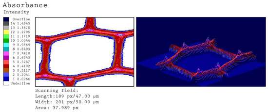
Figure 5.
Representative UV microscopic image profiles of an individual tracheid from reference particle. The colored scale indicates the different UV-absorbance values at a wavelength of 280 nm.
The scanning profile of the untreated spruce tracheids reveals the typical absorbance of lignified cell walls in softwoods. The thick S2 layer of the tracheids is characterized by relatively uniform UV absorbance at 280 nm in the range of 0.20–0.30. The CML and CC of the individual cells can be distinguished on account of significantly higher UV absorbance in the range of 0.40–0.50 (CML) and 0.70–0.80 (CC).
The scanning profile of the adhesive-covered sample (Figure 6) reveals almost identical results for the different cell wall layers. The local deposition of AdCL on the cell wall is emphasized by a significantly higher absorbance (up to 1.3) as compared to the cell wall-associated lignin. These results confirm earlier and recent findings [35,36,37,41].
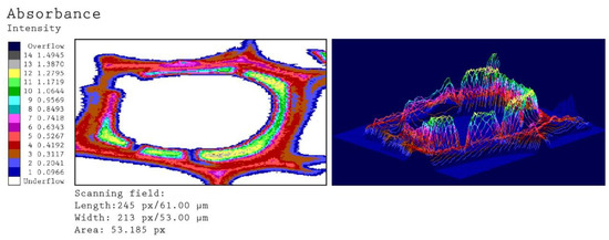
Figure 6.
Representative UV microscopic image profiles of an individual tracheid from adhesive-covered sample. The colored scale indicates the different UV-absorbance values at a wavelength of 280 nm.
In the sample cross-sections examined by light microscopy, only cell lumina in the outer areas of the sample or in the area of cell wall lesions were infiltrated with adhesive. Therefore, it must be assumed that the adhesive could only penetrate through capillary axial action or through destroyed tissue. Penetration via the natural cell wall structure, such as the pits, could not be detected.
3.5.2. Localization of Phenolic Adhesive by Means of Point Measurements
The UV spectra of the S2 and CML show a typical absorbance behavior of softwood lignin with a distinct maximum at 280 nm and local minimum at about 250 nm [36,41]. The deposited phenolic compounds (attached to the cell walls) are characterized by significantly higher absorbance values (log abs 280 nm 1.30) than cell wall-associated lignins (log abs 280 nm 0.20 and 0.70). Furthermore, their absorbance maxima show a bathochromic shift to a wavelength of 290 nm and distinct shoulder in a wavelength range of 340 nm (shown in Figure 7 and Figure 8). This spectral behavior is based on the occurrence of chromophoric groups, particularly conjugated double bonds of condensed phenolics. The higher amount of conjugation stabilizes π–π∗ transitions, which shows characteristic absorbance bands in the range of higher wavelengths [42], clearly detectable by UMSP.
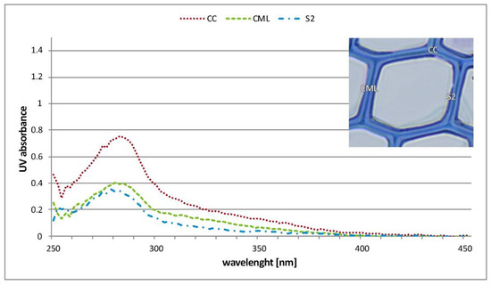
Figure 7.
UV absorbance spectra of individual cell wall layers in the wooden tissue of PM 1 (AC 0%) (CC—cell corner, CML—compound middle lamella, S2—secondary wall).

Figure 8.
UV absorbance spectra of individual cell wall layers and cell lumen-deposited phenolic adhesive in the wooden tissue of PM 3 (AC 19%) (CC—cell corner, CML—compound middle lamella, S2—secondary wall, AdCL1 and AdCL2—adhesives attached to cell lumen).
3.6. Adhesive Detection under Digital Reflected Light Microscope on Particle Surface
The adhesive on the surface of the individual particles is visually very clearly distinguishable from the non-adhesive surface using this technique. Individual particles from PM 2 (AC 8%) and PM 3 (AC 19%) are shown as examples in Figure 9 and Figure 10, respectively. In each case, a particle with the lowest SC, an intermediate SC, and the highest SC is revealed for the nine sieve fractions. The pictures of all imaged particles may be found in the Supplementary Materials file (PDF document). With an AC of 8%, the individual SC on the particles varies between 3 and 76% across all sieve fractions. The particles with an AC of 19% also show a high variation of SC between 9 and 88%. The individual values for the SC of the particles thus show an enormous variance. Low SC particles are found for all particle sizes. A high SC is found with small particle sizes, but not with larger particle sizes. As particle size decreases, larger SC rates are found. That is especially true for particles with a low, (8%) but also with a high (19%), degree of adhesive application. This observation could support the theories about “adhesive-consuming” smallest particles [23].
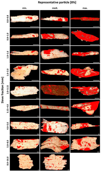
Figure 9.
Particles Material 2 (AC 8%). For each of the first eight sieve fractions, a particle with the lowest degree of surface coverage, an intermediate degree of surface coverage and the highest degree of surface coverage. For the largest sieve fraction, only two particles were available for evaluation. Scale 1000 µm.
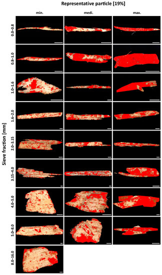
Figure 10.
Particle Material 3 (AC 19%). For each of the first eight sieve fractions, a particle with the lowest degree of surface coverage, an intermediate degree of surface coverage, and the highest degree of surface coverage. For the largest sieve fraction, only one particle was available for evaluation. Scale 1000 µm.
Looking at the mean values only, it suggests an increase in SC with decreasing particle size (Figure 11 and Figure 12). Only the smallest sieve fraction (<0.8 mm) does not follow this trend. Here, in both cases, there was a significantly lower mean value compared to the next largest wire fraction.
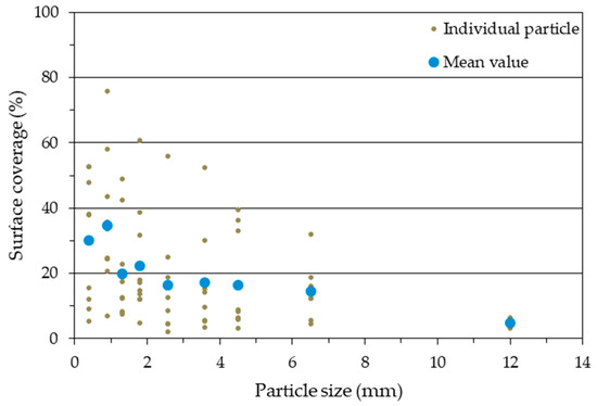
Figure 11.
Mean and individual values of the surface coverage of the individual particles from PM 2 (AC 8%).
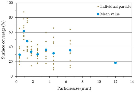
Figure 12.
Mean and individual values of the surface coverage of individual particles from PM 3 (AC 19%).
Tiny individual areas were also detected on PM 1 (AC 0%) as supposed adhesive areas due to their dark coloring (see Supplementary Materials, Excel file). These were probably impurities from the manufacturing process of the particles, such as bark residues. The calculated SC, however, was 0% with one exception (SC 1%).
3.7. Surface-Specific Adhesive Amount When Considering Only a Selection of Sieve Fractions
If only a selection of sieve fractions (0.8–1 mm … 8–16 mm or 1–1.6 mm … 8–16 mm) is considered for the calculation of the surface-specific adhesive amount, this is 10.9 g/m2 (at AC 8%) and 25.9 g/m2 (at AC 19%) in the case of considering the fractions 0.8–1 mm … 8–16 mm, and 11.3 g/m2 (at AC 8%) and 26.9 g/m2 (at AC 19%) in the case of considering the fractions 1–1.6 mm … 8–16 mm.
- Fractions 0.8–1 mm … 8–16 mm considered:
- (126.7 g × 8%)/0.93 m2 = 10.9 g/m2;
- (126.7 g × 19%)/0.93 m2 = 25.9 g/m2.
- Fractions 1–1.6 mm … 8–16 mm considered:
- (122.5 g × 8%)/0.87 m2 = 11.3 g/m2;
- (122.5 g × 19%)/0.87 m2 = 26.9 g/m2.
The fact that the surface-specific adhesive amount increases with decreasing relative particle surface for unchanged adhesive content is quite logical and suggests that more adhesive is available on the particle surface for bonding the wood particles to each other. For industrial practice, however, it is less interesting how high the surface wetting is with unchanged adhesive content, but rather to which adhesive content can be reduced with unchanged surface wetting.
3.8. Adhesive Content with Unchanged SSAA and Consideration of Only Selected Sieve Fractions
If only a selection of sieve fractions (0.8–1 mm … 8–16 mm or 1–1.6 mm … 8–16 mm) is considered and the surface-specific adhesive amount is kept at the level of Particle Material 1 (10.3 g/m2 or 24.4 g/m2), the adhesive content is 7.5% or 17.9% in the case of considering the fractions 0.8–1 mm … >8 mm, and 7.3% or 17.2% in the case of considering the fractions 1–1.6 mm … 8–16 mm.
- Fractions 0.8–1 mm … 8–16 mm considered:
- 10.3 g/m2 × 0.93 m2 = 9.5 g; 9.5 g/126.7 g × 100 = 7.5%;
- 24.4 g/m2 × 0.93 m2 = 22.7 g; 22.7 g/126.7 g × 100 = 17.9%.
- Fractions 1–1.6 mm … 8–16 mm considered:
- 10.3 g/m2 × 0.87 m2 = 8.9 g; 8.9 g/122.5 g × 100 = 7.3%;
- 24.4 g/m2 × 0.87 m2 = 21.1 g; 21.1 g/122.5 g × 100 = 17.2%.
This shows that the adhesive content can be reduced when sorting out the fine fractions, i.e., adhesive can be saved without reducing the surface wetting.
3.9. Calculation of Prices Based on Data from Aßmann (2015)
Following Equation (4), the particle mass per cubic meter model particleboard (parameters given in Materials and Methods) is calculated as 540 kg/m3 (face layers: 186 kg/m3, core layer: 354 kg/m3). The adhesive mass was calculated as 49 kg/m3 (20.5 kg/m3 + 28.3 kg/m3). This means an adhesive content over the entire board of 9% (49 kg/m3/540 kg/m3). In connection with the data from Aßmann (2015) [1] for wood (48 €/m3), particle preparation (20 €/m3), and adhesive (23 €/m3), prices result in the amount of 89 €/t wood, 37 €/t particle preparation, and 311 €/t (472 €/t solid) adhesive. Currently, prices for adhesive emulsion are assumed to be 560–580 €/t [43] (mean value 570 €/t), which corresponds to costs of 864 €/t solid adhesive.
3.10. Calculation of Possible Savings through the Use of Selected Sieve Fractions
For the calculation of the possible savings through the use of selected sieve fractions, first, the wood mass in the example particleboard has to be calculated in respect to the relevant adhesive content following Equation (4) and amounts to
- AC 8%: 545 kg/m3;
- AC 7.5%: 547 kg/m3;
- AC 7.3%: 549 kg/m3;
- AC 19%: 492 kg/m3;
- AC 17.9%: 497 kg/m3;
- AC 17.2%: 500 kg/m3.
Furthermore, the factor is to be calculated by which the wood mass in the board is to be increased in order to obtain the wood mass needed:
- f 0.8–1mm…>8mm = 131.2 g/126.7 g = 1.036;
- f 1–1.6mm…>8mm = 131.2 g/122.5 g = 1.071.
The additional demand in particles is calculated as
- (547 kg/m3 × 1.036) − 545 kg/m3 = 22 kg/m3;
- (549 kg/m3 × 1.071) − 545 kg/m3 = 43 kg/m3;
- (497 kg/m3 × 1.036) − 492 kg/m3 = 23 kg/m3;
- (500 kg/m3 × 1.071) − 492 kg/m3 = 43 kg/m3;
and the savings on adhesive as
- 547 kg/m3 × 7.5% − 545 kg/m3 × 8% = 2.3 kg/m3;
- 549 kg/m3 × 17.9% − 545 kg/m3 × 8% = 3.8 kg/m3;
- 497 kg/m3 × 7.3% − 545 kg/m3 × 8% = 4.6 kg/m3;
- 500 kg/m3 × 17.2% − 545 kg/m3 × 8% = 7.3 kg/m3.
Table 4 provides an overview of the results up to this point.
Table 4.
Results overview.
Combining the results of the possible savings or the additional expense by quantity with the material prices (particles 126 €/t, adhesive 864 €/t), the possible financial savings from using a selection of particle fractions can be estimated. Thus, sorting out the smallest (<0.8 mm) sieve fraction (of the two smallest (<0.8 mm and 0.8–1.0 mm) sieve fractions) would mean additional costs for particles of 2.85 €/m3 (5.47 €/m3), in return for a cost saving for adhesive of 3.95 €/m3 (6.34 €/m3) and thus a total saving of 1.10 €/m3 (0.87 €/m3) for an adhesive content of 19%. With an adhesive content of 8%, assuming a uniform adhesive distribution over the particle surface regardless of the particle size, there is no cost saving:
- Smallest fraction (<0.8 mm) sieved out
- Additional cost for particles 2.78 €/m3;
- Saving for adhesive 2.03 €/m3;
- Total saving −0.75 €/m3 (which means additional expenses).
- Two smallest fractions (<0.8 mm and 0.8–1.0 mm) sieved out
- Additional cost for particles 5.44 €/m3;
- Saving for adhesive 3.25 €/m3;
- Total saving −2.19 €/m3 (which means additional expenses).
4. Discussion
Similar to what Dunky (1988) [23] showed at the end of the 1980s for a fictitious data set, an increase in the fraction mass-specific particle surface area with decreasing particle size was observed for a real data set (sieve-fractionated, 3D-measured core layer particles) in the present paper. Assuming a uniform surface-specific adhesive amount across all fractions, the same applies to the adhesive content, which increases with decreasing particle size for both the fictitious and the real data set.
For the data from source [23], this is not surprising, since the number of particles was selected to increase with decreasing particle size and the particle surface area for each fraction (Fi) was calculated for uniform fraction masses of about 100 g, as can be calculated from the data given in Table 5 and the formula (Equation (7)) that Dunky provided in source [23].
Ni = (103 × mHi)/(δ × li × bi × di) ↔ mHi = (Ni × δ × li × bi × di)/103
Table 5.
Selection from the fictitious data set given and used by Dunky (1988) [23].
Here, mHi is the particle amount in the fraction (g); Ni is the number of particles in the fraction; δ is the wood density (g/cm3)—here, a value of 0.5 was assumed, similar to that of Scots pine; li is the particle length (mm); bi is the particle width (mm); di is the particle thickness (mm).
For the data of the present study, an increase in the fraction mass-specific particle surface area with decreasing particle size (Table 3 and Figure 3) is not surprising, due to the well-known relationship of surface area and volume of geometric bodies (surface-to-volume ratio). The same applies for increasing adhesive content with decreasing particle size (Figure 4), since the mass of adhesive is calculated based on a uniform surface-specific adhesive amount and related to the mass of the fraction.
However, it is of practical importance, for example, for particleboard production, how the absolute amount of adhesive per fraction relates to its contribution to the board formation (e.g., strength or volume). Finally, the absolute number of particles or the absolute particle mass does not necessarily increase with decreasing particle size. Instead, the mass and surface distribution often resemble a normal or logarithmic normal distribution, as Figure 13 for PM 1 shows. This means that the absolute adhesive amount decreases again with decreasing particle size after a maximum.
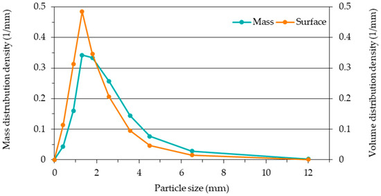
Figure 13.
Mass and surface distribution density for particles, according to their size, of Particle Material 1.
Table 6.
Data used to create Figure 13.
However, assuming that fine particles have an adhesive-consuming character and contribute little to the structure and strength of the board, one must consider whether the adhesive bonded here could not make a greater contribution elsewhere, or whether a cost advantage could be achieved by partially saving at the expense of a higher overall particle requirement. This was achieved in the present work based on the results of determining the total particle surface area of sieve fractions with 3D Particleview and price data for particles and adhesive [1,43].
It was shown that by sorting out the smallest (<0.8 mm) fraction (the two smallest (<0.8 mm and 0.8–1.0 mm) sieve fractions) in the case of 19% adhesive content, a total saving of 1.10 €/m3 (0.87 €/m3) would be achieved. In the case of an adhesive content of 8%, the procedure is not associated with cost savings if a uniform adhesive distribution over the particle surface is assumed regardless of the particle size.
However, the approach chosen did not consider the microscopic investigations which have shown that the surface coverage with adhesive tends to be higher for fine particles (except the smallest (<0.8 mm) sieve fraction) than for coarse particles. One reason for the low SC of the smallest (<0.8 mm) sieve fraction (Figure 11 and Figure 12) could be that small particles with high SC tend to clump with other particles and are thus no longer present as small particles with high SC. This explanation is also supported by the results of the sieve analysis (Table 2). The result here was that the particle size distribution shifted to the right, toward coarser particles, as the degree of gluing increased.
If the adhesive were not assumed to be uniformly distributed over the particle surface, but rather assigned to the fractions via the surface coverage, cost savings would result from screening out the fines even for adhesive amounts considerably lower than 19%. Furthermore, if it is assumed that coarse particles take up more load than the fines, and consequently the board density could be reduced, further material and thus cost savings would be possible. This consideration does not consider the fact that the fine particles to be sieved out could be used for other purposes (e.g., energy production) and would thus have a positive impact on the costs of this approach.
In the present work, as already mentioned at the beginning, PF adhesive with appropriate visibility was deliberately used. Of course, the research on the widely used UF adhesive is much closer to reality. CLSM seems to be a promising technique to visualize the diffusion of colloidal adhesives. The fluorescence of the individual materials plays a crucial role here, whereas there is presently no proof of widespread fluorescence recovery after photo bleaching (FRAP) applicability in colloidal science [44].
New automated techniques (for example, machine learning) are becoming available for future characterization of adhesive distribution on particles or within a particleboard. These conduct the analysis of the available image data faster and often more accurately. However, the success of machine learning systems is very much dependent on the data sets available for training the neural networks used.
Supplementary Materials
The following supporting information can be downloaded at: http://www.mdpi.com/article/10.3390/fib10110097/s1, Excel file: Raw Data; PDF document: Pictures of all imaged particles.
Author Contributions
Conceptualization, J.T.B., J.S.-R. and J.L.; Formal Analysis, J.T.B., J.S.-R. and G.K.; Investigation, J.T.B., J.S.-R. and N.E.; Writing—Original Draft, J.T.B., J.S.-R. and N.E.; Writing—Review and Editing, J.T.B., J.S.-R., N.E., J.L. and G.K.; Visualization, J.T.B. and J.S.-R.; Project Administration, J.T.B. All authors have read and agreed to the published version of the manuscript.
Funding
This research received no external funding.
Institutional Review Board Statement
Not applicable.
Informed Consent Statement
Not applicable.
Data Availability Statement
The data presented in this study are included in the article or have been made available through the Supplementary Material.
Acknowledgments
The authors would like to thank all those colleagues who were engaged in the experimental realization and data analysis, namely, Sabrina Heldner, Sergej Kaschuro, Tim Lewandrowski, Daniela Paul, Tanja Potsch, Bettina Steffen (all Thünen Institute of Wood Research), and Christina Waitkus (Thünen Institute, Photography).
Conflicts of Interest
The authors declare no conflict of interest.
References
- Aßmann, J. Kostendruck macht erfinderisch [Cost pressure makes inventive]. In Proceedings of the 11. Holzwerkstoffkolloquium, Dresden, Germany, 10–12 December 2015. [Google Scholar]
- Niemz, P. Grundlagen [Basics]. In Holzwerkstoffe und Leime—Technologie und Einflussfaktoren [Wood-Based Materials and Adhesives–Technology and Influencing Factors]; Dunky, M., Niemz, P., Eds.; Springer: Berlin/Heidelberg, Germany, 2002; pp. 1–243. ISBN 978-3-642-55938-9. [Google Scholar]
- Irle, M.; Barbu, M.C. Wood-Based Panel Technology. In Wood-Based Panels—An Introduction for Specialists; Thoemen, H., Irle, M., Sernek, M., Eds.; Brunel University Press: London, UK, 2010; pp. 1–94. [Google Scholar]
- Food and Agriculture Organization of the United Nations (FAO), FAOSTAT, Forestry, Forestry Production and Trade. Available online: https://www.fao.org/faostat/en/#data/FO (accessed on 7 December 2020).
- European Panel Federation (EPF). Annual Report 2019–2020; EPF: Brussels, Belgium, 2020; p. 346. [Google Scholar]
- Klauditz, W.; Stegmann, G. Über die Eignung von Pappelholz zur Herstellung von Holzspanplatten [About the suitability of poplar wood for the production of particleboards]. Holzforschung 1957, 11, 174–179. [Google Scholar]
- Plath, E. Einfluß der Rohdichte auf die Eigenschaften von Holzwerkstoffen–Influence of Density on the Properties of Wood-based Materials. Holz Roh Werkst. 1963, 21, 104–108. [Google Scholar] [CrossRef]
- Liiri, O. Investigations on properties of wood particle boards. Paperi Puu 1961, 43, 3–18. [Google Scholar]
- Istek, A.; Siradag, H. The effect of density on particleboard properties. In Proceedings of the International Caucasian Forestry Symposium (ICFS), Artvin, Turkey, 25–26 October 2013; pp. 932–938. [Google Scholar]
- Benthien, J.T.; Ohlmeyer, M. Influence of face-to-core layer ratio and core layer resin content on the properties of density-decreased particleboards. Eur. J. Wood Wood Prod. 2017, 75, 55–62. [Google Scholar] [CrossRef]
- Walter, K.; Kieser, J.; Wittke, T. Einfluss der Spanform auf einige Festigkeitseigenschaften orientiert gestreuter Spanplatten [Effect of chip size on some strength properties of oriented structural board]. Holz Roh Werkst. 1979, 37, 183–188. [Google Scholar] [CrossRef]
- May, H.A. Herstellung von Holzspanlatten mit orientierten Spänen und unterschiedlicher Formgebung [Manufacture of particle board with oriented chips and different types of formation]. Holz Roh Werkst. 1974, 32, 169–176. [Google Scholar] [CrossRef]
- Wong, E.D.; Zhang, M.; Wang, Q.; Kawai, S. Formation of the density profile and its effects on the properties of particleboard. Wood Sci. Technol. 1999, 33, 327–340. [Google Scholar] [CrossRef]
- Dunky, M. Einflussgrößen [Influencing variables]. In Holzwerkstoffe und Leime–Technologie und Einflussfaktoren [Wood-Based Materials and Adhesives–Technology and Influencing Factors]; Dunky, M., Niemz, P., Eds.; Springer: Berlin/Heidelberg, Germany, 2002; pp. 645–927. ISBN 978-3-642-55938-9. [Google Scholar]
- Benthien, J.T.; Heldner, S.; Lüdtke, J. Spandicke bildanalytisch messen–Thünen-Institut für Holzforschung und Grecon entwickeln System zur 3D-Vermessung von Spänen [Measuring chip thickness by image analysis-Thünen Institute for Wood Research and Grecon develop system for 3D measurement of chips]. Holz-Zent 2019, 38, 800. [Google Scholar]
- Warmbier, K.; Wilczynski, M. Resin Content and Board Density Dependent Mechanical Properties of One-Layer Particleboard Made from Willow (Salix viminalis). Drvna Ind. 2016, 67, 127–131. [Google Scholar] [CrossRef]
- Galilei, G. Unterredungen und Mathematische Demonstrationen über Zwei Neue Wissenszweige, die Mechanik und die Fallgesetze Betreffend (Erster und Zweiter Tag) [Conversations and Mathematical Demonstrations on Two New Branches of Knowledge, Concerning Mechanics and the Laws of Falling Bodies (First and Second Day)]; Wilhelm Engelmann: Leipzig, Germany, 1890; p. 142. [Google Scholar]
- Benthien, J.T.; Ohlmeyer, M. Zusammenhang von Spanqualität und Platteneigenschaften—Eine Untersuchung von Spänen Verschiedener Hersteller [Relationship between Particle Quality and Board Properties-An Investigation of Particles from Different Manufacturers]; Thünen Working Paper 52; Johann Heinrich von Thünen-Institut: Braunschweig, Germany, 2016; p. 38. [Google Scholar] [CrossRef]
- Istek, A.; Aydin, U.; Özlüsoylu, I. The effect of chip size on the particleboard properties. In Proceedings of the International Congress on Engineering and Life Science (ICELIS), Kastamouno, Turkey, 26–29 April 2018; pp. 439–444. [Google Scholar]
- Kitahara, K.; Kasagi, K. Effects of raw chip dimensions on the physical and mechanical properties of chip-board. Wood Ind. 1955, 10, 406–412. [Google Scholar]
- Deppe, H.J.; Ernst, K. Taschenbuch der Spanplattentechnik [Pocketbook of Chipboard Technology], 4th ed.; DRW: Leinfelder-Echterdingen, Germany, 2000; p. 552. [Google Scholar]
- Marhenke, T.; Hasener, J. Späne lügen nicht [Particles don’t lie]. MDF Magazin, 04 October 2019; 78–82. [Google Scholar]
- Dunky, M. Einfluss der Spangrößenverteilung auf den Beleimungsgrad der Späne [Infuence of the particle size distribution on the particles’ resin content]. Holzforsch. Holzverwert. 1988, 40, 126–133. [Google Scholar]
- Dunky, M. Particleboard Size Distribution and Glue Resin Consumption: How to Spare Costs. In Proceedings of the Second European Panel Products Symposium, Wales, UK, 21–22 October 1998; pp. 206–217. [Google Scholar]
- Pichelin, F.; Dunky, M. Technique of Application of the Resin on Particles and Strands. In COST Action E13–Wood Adhesion and Glued Products–Working Group 1: Wood Adhesives–State of the Art–Report, 1st ed.; Dunky, M., Pizzi, T., Van Leemput, M., Eds.; Office for Official Publications of the European Communities: Luxembourg, 2003; pp. 98–102. [Google Scholar]
- Meinecke, E.; Klauditz, W. Über die Physikalischen und Technischen Vorgänge bei der Beleimung und Verleimung von Holzspänen bei der Herstellung von Holzspanplatten [On the Physical and Technical Processes in the Gluing and Bonding of Wood Chips in the Manufacture of Particleboards]; Forschungsbericht Nr. 1053 des Landes Nordrhein-Westfalen [Research Report No. 1053 of the Federal State of North Rhine-Westphalia]; Westdeutscher: Cologne, Germany, 1962. [Google Scholar]
- Hill, M.D.; Wilson, J.B. Particleboard Strength as Affected by Unequal Resin Distribution on Different Particle Fractions. Forest Prod. J. 1978, 28, 44–48. [Google Scholar]
- Eusebio, G.A.; Generalla, N.C. Effect of particle resin adhesive distribution in particleboard manufacture of Kaatoan Bangkal [Anthocephalus chinensis (Lam.) Rich. ex Walp.]. FPRDI J. 1983, 12, 12–19. [Google Scholar]
- Medved, S.; Grudnik, J. Influence of resin content on the surface covered with adhesive. Int. J. Adhes. Adhes. 2021, 104, 102698. [Google Scholar] [CrossRef]
- Ducan, T.F. Normal Resin Distribution in Particleboard Manufacture. Forest Prod. J. 1974, 24, 36–44. [Google Scholar]
- Zhu, P.; Moran-Mirabal, J.M.; Luterbacher, J.S.; Walker, L.P.; Craighead, H.G. Observing Thermobifida fusca cellulase binding to pretreated wood particles using time-lapse confocal laser scanning microscopy. Cellulose 2011, 18, 749–758. [Google Scholar] [CrossRef]
- Altgen, D.; Grigsby, W.; Altgen, M.; Rautkari, L.; Mai, C. Analyzing the UF resin distribution in particleboards by confocal laser scanning microscopy. Compos. Part A Appl. Sci. Manuf. 2019, 125, 105529. [Google Scholar] [CrossRef]
- Brady, D.E.; Kamke, F.A. Effect of hot-pressing parameters on resin penetration. Forest Prod. J. 1988, 38, 63–68. [Google Scholar]
- Biziks, V.; Bicke, S.; Koch, G.; Militz, H. Effect of phenol-formaldehyde (PF) resin oligomer size on the decay resistance of beech wood. Holzforschung 2021, 75, 574–583. [Google Scholar] [CrossRef]
- Koch, G.; Kleist, G. Application of scanning UV microspectrophotometry to localise lignins and phenolic extractives in plant cell walls. Holzforschung 2001, 55, 563–567. [Google Scholar] [CrossRef]
- Koch, G.; Grünwald, C. Application of UV microspectrophotometry for the topochemical detection of lignin and phenolic extractives in wood fibre cell walls. In Wood Fibre Cell Walls: Methods to Study Their Formation, Structure and Properties; Schmitt, U., Ander, P., Barnett, J.R., Emons, A.M.C., Jeronimidis, G., Saranpää, P., Tschegg, S., Eds.; Swedish University of Agricultural Sciences: Uppsala, Sweden, 2004; pp. 119–130. [Google Scholar]
- Koch, G.; Richter, H.G.; Schmitt, U. Topochemical investigation on phenolic deposits in the vessels of afzelia (Afzelia spp.) and merbau (Intsia spp.) heartwood. Holzforschung 2006, 60, 583–588. [Google Scholar] [CrossRef]
- Benthien, J.T.; Ohlmeyer, M. Effects of flat-shaped face layer particles and core layer particles of intentionally greater thickness on the properties of wood-reduced particleboard. MDPI Fibers 2020, 8, 46. [Google Scholar] [CrossRef]
- Spurr, A.R. A low viscosity epoxy resin embedding medium for electron microscopy. J. Ultrastruct. Res. 1969, 26, 31–43. [Google Scholar] [CrossRef]
- Kleist, G.; Schmitt, U. Evidence of accessory components in vessel walls of Sapelli heartwood (Entandrophragma cylindricum) obtained by transmission electron microscopy. Holz Roh Werkst. 1999, 57, 93–95. [Google Scholar] [CrossRef]
- Fergus, B.J.; Procter, A.R.; Scott, J.A.N.; Goring, D.A.I. The distribution of lignin in sprucewood as determined by ultraviolet microscopy. Wood Sci. Technol. 1969, 3, 117–138. [Google Scholar] [CrossRef]
- Goldschmid, O. Ultraviolet spectra. In Lignins, Occurrence, Formation, Structure and Reactions; Sarkanen, K.V., Ludwig, C.H., Eds.; Wiley Interscience: New York, NY, USA, 1971; pp. 241–266. [Google Scholar] [CrossRef]
- Anonymous. Anstieg der Harzpreise hat sich im Oktober verstärkt/Leim- und Imprägnierharzpreise werden in kurzen Abständen angepasst [Rise in resin prices intensified in October/Glue and impregnating resin prices are adjusted at short interval]. Euwid Holz Holzwerkst. 2021, 21. [Google Scholar]
- Moud, A.A. Fluorescence Recovery after Photobleaching in Colloidal Science: Introduction and Application. ACS Biomater. Sci. Eng. 2022, 8, 1028–1048. [Google Scholar] [CrossRef]
Publisher’s Note: MDPI stays neutral with regard to jurisdictional claims in published maps and institutional affiliations. |
© 2022 by the authors. Licensee MDPI, Basel, Switzerland. This article is an open access article distributed under the terms and conditions of the Creative Commons Attribution (CC BY) license (https://creativecommons.org/licenses/by/4.0/).