Abstract
A disadvantage of using linear polarization resistance (LPR) in the measurement of corrosion current density is the need to partially destroy a concrete cover. In this article, a new technique of predicting the corrosion current density in reinforced concrete using a self-organizing feature map (SOFM) is presented. For this purpose, air temperature, and also the parameters determined by the resistivity four-probe method and galvanostatic resistivity measurements, were employed as input variables. The corrosion current density, predicted by the destructive LPR method, was employed as the output variable. The weights of the SOFM were optimized using the genetic algorithm (GA). To evaluate the accuracy of the SOFM, a comparison with the radial basis function (RBF) and linear regression (LR) was performed. The results indicate that the SOFM–GA model has a higher ability, flexibility, and accuracy than the RBF and LR.
1. Introduction
Corrosion of steel reinforcements has recently become a major problem in civil engineering [1,2,3]. Thus, the attention of researchers is nowadays devoted to the protection of concrete and steel reinforcements against corrosion [4,5,6,7]. One of the main issues of this protection is the proper prediction of the corrosion rate [8,9,10,11,12,13]. A direct method of providing an evaluation of the corrosion rate based on a corrosion current density (icorr) measurement is linear polarization resistance (LPR). In LPR method a small direct current (DC) electrical signal (ΔI) is introduced to a steel reinforcement bar. A surface electrode is applied for this purpose (Figure 1a).
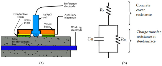
Figure 1.
Scheme of (a) linear polarisation resistance measurement (LPR) and (b) Randle’s equivalent electrical circuit [19].
When a suitable time for equilibrium is established, the change in potential (ΔE) is measured and the polarisation resistance (Rp) is given by the Stern-Geary Equation [14]:
An equivalent electrical Randle’s circuit can be used to model corrosion process [15]. According to Figure 1b Randle’s circuit consists of a concrete cover resistance (Rp) with the combination of the double-layer capacitance (Cdl) and a charge transfer resistance (Rct):
where Rs is the concrete cover resistance. Finally, the icorr is given by:
where B is a Stern-Geary proportionality constant [16] and A is the area of steel being perturbed. A disadvantage of using the LPR method for a corrosion current density measurement is that it requires the partial destruction of a concrete cover in order to provide an electrical connection to the steel [17,18]. To avoid this shortcoming in [19] the proposal of a new corrosion rate assessment method was offered. The principle of this model is primary to take a four-point resistivity measurement using an alternating current (AC) passed through Cdl (Figure 1b). Thus, the resistivity first is measured over (ρAC,bar) or away (ρAC,conc) from the steel bar. Then, the same measurement has to be taken once more using a DC current to measure the resistivity ρDC.
In the last few years, artificial neural networks (ANNs) have emerged as powerful devices that can be used in many civil engineering applications [20,21,22,23,24,25]. Thus, researchers have developed a series of models of steel corrosion using an ANN [26,27,28,29,30,31,32]. In previous research, ANN models based on a conventional multilayer perceptron (MLP) were established [33]. These models have a theoretical value as they can predict the corrosion current density without the need for a connection to the steel reinforcement. The MLP has a satisfactory performance for reinforced concrete slabs with a high corrosion rate (R2 = 0.9436 for training and R2 = 0.9843 for testing), while the observed performance for reinforced concrete slabs with a moderate corrosion rate was lower (R2 around 0.9109 for training and 0.9801 for testing). Considering the above, the imperialist competitive algorithm (ICA) was used, but the obtained values of determination coefficients R2 of around 0.8019 and 0.9045 (for training and testing, respectively) were not satisfactory [34].
It should be noted that a great deal of progress has been made in the field of artificial intelligence modelling in the last few years. One result of this progress is the self-organizing feature map (SOFM). The SOFM was established by Kohonen [35,36] and described in detail [37,38]. The SOFM is developed based on the unique nature of the human brain and its specific characteristics. In a SOFM, processing units are placed in nodes of multi-dimensional networks (usually one-dimensional or two-dimensional, as indicated in Figure 2). The learning process is competitive. The obtained coordinate system forms a topographic map of input patterns in order to compete with each other at each step of learning. Only one unit wins at the end of this competition [35]. The total weight of the entries in various units come out of an output [36,38,39,40]. Recently, the SOFM has become more frequently used when solving civil engineering problems [41,42,43,44,45]. In this research, better prediction results are more probable with the use of the SOFM than with the use of previous models.
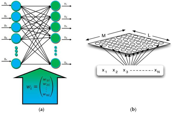
Figure 2.
Model of (a) a one-dimensional structural model of the SOFM [35] and (b) a two-dimensional structural model of the SOFM [45].
Considering the above, the article presents a new technique of predicting the corrosion current density in reinforced concrete using a SOFM. For this purpose, air temperature and also parameters determined by the resistivity four-probe method and galvanostatic resistivity measurements were employed as inputs. The corrosion current density, predicted by the destructive LPR method, was employed as the output. The weights of the SOFM were optimized using the genetic algorithm (GA). To evaluate the accuracy of the SOFM, a comparison with the radial basis function (RBF) and linear regression (LR) was performed.
2. Experimental Setup
Reinforced concrete slab specimens with dimensions 400 mm × 300 mm × 100 mm were prepared. Each specimen contained a single steel bar with the diameter equal to 30 mm. The steel bar was made from class A–III grade 34GS steel. The concrete cover was equal to 20 mm. The reinforced concrete slabs were made from class C 20/25 concrete. The concrete was composed of Portland cement CEM I 42.5R. The coarse aggregate with a maximum grain size Dmax of 8 mm has been used.
The specimens were corroded in natural environment. Then the samples were stored in laboratory conditions: the ambient air temperature of 20 °C (±1 °C) and an air relative humidity of 65% (±1%). The AC resistivity measurements were performed on two positions: directly over the bar (Position 1) and away the bar (Position 2), as presented in Figure 3b. As described in [19], a modified electrode array was used to perform DC resistivity measurements (at Position 1). For this purpose, two copper-copper sulphate reference electrodes were used to replace the two inner standard resistivity probes (Figure 3a). Repeated measurements were taken over several days. Then, LPR method has been applied to measure the actual icorr. The exemplary data were presented in Table 1.
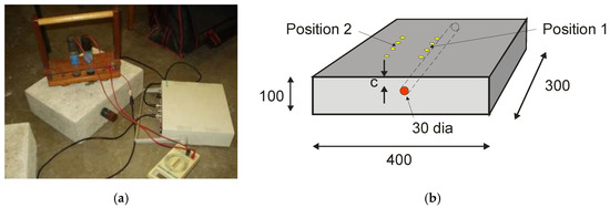
Figure 3.
Scheme of (a) DC resistivity equipment on reinforced concrete specimen and (b) resistivity measurement locations on concrete specimen [19].

Table 1.
Exemplary steel corrosion data with moderate corrosion rates [33].
The statistical characteristics of the database are summarized in Table 2. As presented in Table 2 bar had an icorr between 0.37 and 0.49 μA/cm2 with the coefficient of variation of 7.09%. Judging by this, the conditions have been steady and close to passivity. They are low compared to others [46,47]. The measured air temperature T during the investigations was 20 °C (±1 °C) with the coefficient of variation equal to 3.28%. The resistivity measurements exhibits low scatter with coefficient of variation below 1% (Table 2). The Shapiro-Wilk compliance test with normal distribution was also conducted (Table 3), in accordance with [48]. In this test the hypothesis of compliance with normal distribution is rejected, if the level of W probability is lower than the determined probability Wn(α) under the level of the significance (α).
Table 2.
Statistical characteristics of the database (based on data presented in [33]).
Table 3.
Results of the Shapiro-Wilk test.
For α = 0.01, the hypothesis regarding compliance of the distribution of all the parameters with normal distribution desires to be rejected for T, ρAC,conc and ρDC (Table 3). Thus, the most useful input parameter will be the ρAC,bar and icorr as an output variable. Then, the correlations between the input parameters and icorr, were investigated using Pearson’s (p), Spearmann’s (ρs) and Kendall’s (τ) correlation coefficients (Figure 4). Parameters are considered to be useful when the values of p, ρs and τ are in a range from ±1 to ±0.4.
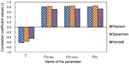
Figure 4.
Pearson’s (p), Spearmann’s (ρs), and Kendall’s (τ) rank correlation coefficient values between input parameters and the icorr.
The correlation coefficients p, ρs and τ obtain the highest value in a range between 0.73 and 0.85 for the resistivity parameters (Figure 4). It may indicate the key importance of these parameters for the SOFM. The negative values of correlation coefficients in the case of parameter T indicate a decrease of their values with an increase of the output variable icorr. The values of coefficients p, ρs and τ obtained in the range between −0.46 and −0.62 affirm the lack of correlation between T and the icorr.
3. Results and Discussion
3.1. Selection of the Optimum Prediction Model Using the SOFM
From the database presented in Table 1, 80% of the samples (54 samples) were used for training, 10% (seven samples) for validation and 10% (seven samples) for testing. Equation (4) was used to determine the number of nodes in the hidden layer (HL) [49]:
where NH is the maximum number of nodes in the HLs and NI is the number of inputs. Considering that the effective number of inputs is equal to 4, the maximum number of nodes in the HL is equal to 9 (Table 4).
Table 4.
Different SOFM models.
For each model the equation has been provided together with the value of the determination coefficient (R2) for training, validation and testing (Table 5). Table 6 presents the errors: mean (ME), mean absolute (MAE), root mean squared (RMSE), and mean squared (MSE). The optimum structure is 1-9-4. The detailed results are then presented in Figure 5 and Figure 6.
Table 5.
Results of the different SOFM models in the training, validation, and testing phases.
Table 6.
Statistical analysis of the different SOFM models in training, validation, and testing.
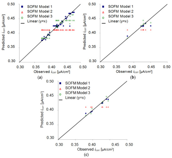
Figure 5.
Corrosion current density prediction using the different SOFM models in the processes of (a) training, (b) validation, and (c) testing.
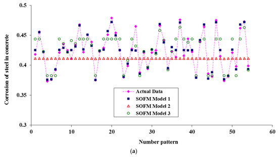
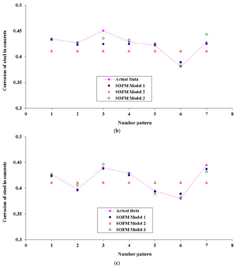
Figure 6.
Comparison of corrosion current density prediction using the different SOFM models in the processes of (a) training, (b) validation, and (c) testing.
3.2. Sensitivity Analysis of the Selected SOFM–GA Model
To determine the effect of input parameters on output parameters, the sensitivity analysis technique is used (Table 7).
Table 7.
Analysis of the sensitivity of the output in the SOFM–GA model in comparison to the input parameters.
According to Table 7, parameters T and ρDC have the least and greatest impact respectively on the output of SOFM–GA Model 1. The best network for matching the input data in the SOFM–GA model is a 5 × 5 structure, which is indicated in Figure 7 for the training, validation, and testing phases.
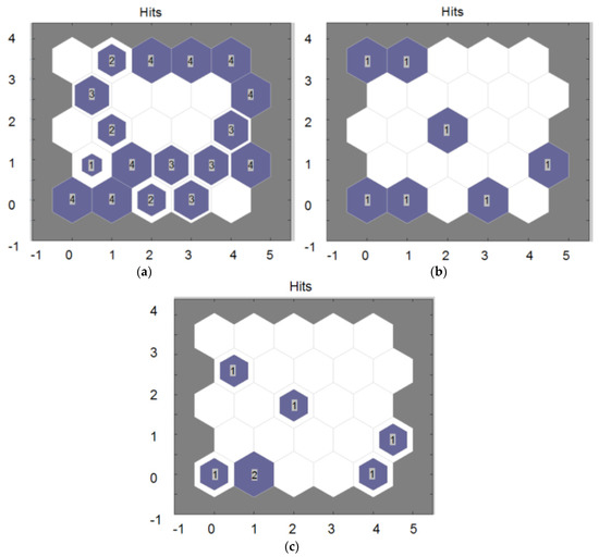
Figure 7.
Structure for matching the input data in the processes of (a) training, (b) validation, and (c) testing.
3.3. Comparison of the Selected SOFM–GA Model with Linear Regression (LR) and the Radial Basis Function (RBF) Neural Network
The SOFM–GA model was compared with LR models and these statistical models are presented in Equations (4)–(6). To determine the statistical equations, MINITAB Student 14 software was used [50]:
| LR 1: | icorr = −9.95 + 0.446ρAC + 0.0792ρAC,conc | (4) |
| LR 2: | icorr = −9.19 + 0.0352ρDC + 0.392ρAC + 0.0577ρAC,conc | (5) |
| LR 3: | icorr = −3.10 − 0.01537T + 0.1143ρDC − 0.049ρAC + 0.1028ρAC,conc | (6) |
The results are shown for four models for the training, validation and testing of data for the statistical indicators in Table 8 and Table 9. Table 8 deals with investigating the results with respect to the straight line slope and the R2, while the statistical indicators are presented in Table 9. The results indicate that LR 3 model is more accurate than the other models.
Table 8.
Results of different models of LR in the training, validation, and testing phases.
Table 9.
Statistical analysis of different models of LR in the training, validation, and testing phases.
For comparing the SOFM–GA model to an ANN, the RBF network was used. NeuroSolutions 5.0 software [51] was used to determine the optimal structure of the RBF model regarding the number of hidden layers, the number of nodes in the hidden layers, the learning algorithm of the network, the transfer function, and the GA. Table 10 indicates the optimal structure of the RBF model. Moreover, Table 11 deals with the results with respect to the indexes of the straight line slope and coefficient of convergence. The statistical indicators are evaluated in Table 12. The results indicate that RBF model 3 shows great and logical accuracy when compared to the other two models.
Table 10.
The structure of different RBF models optimized with the GA.
Table 11.
Results of different RBF models in the training, validation and testing phases.
Table 12.
Statistical analysis of the different RBF models in the training, validation and testing phases.
According to analysis of all the models, the three models of SOFM–GA, LR Model 4, and RBF model 3 were selected as the best and are presented in Table 13 and Table 14.
Table 13.
Results of the different models in training, validation and testing.
Table 14.
Statistical analysis of the different models in training, validation and testing.
According to analysis of the three models, the SOFM–GA has higher precision and flexibility than the other two models and these results are shown in Figure 8.
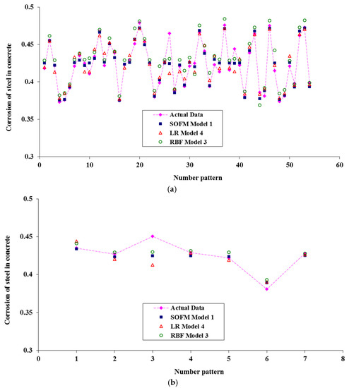
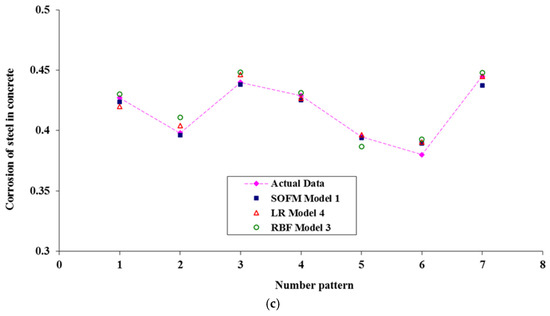
Figure 8.
Comparison of corrosion current density prediction using the different SOFM models in the processes of (a) training, (b) validation, and (c) testing.
4. Conclusions
Based on the research and analysis presented in the article, the following conclusions can be made:
- It is possible to predict corrosion current density using a SOFM that is optimized with the GA on the basis of parameters determined by non-destructive resistivity measurements and temperature monitoring.
- The GA optimization feature can be used as a powerful tool for optimizing the weights of a SOFM.
- When comparing the results of training, validation and testing of different models of a SOFM, it can be seen that the SOFM model with a 1-9-4 structure, transfer function of TanhAxon, and a momentum training algorithm has a higher ability and accuracy in predicting the corrosion current density of steel in concrete.
- In the SOFM–GA model, the determination coefficient R2 in the training, validation and testing phases is respectively 0.9333, 0.924, and 0.9786, and the slope of the straight line for this parameter is equal to 0.9292, 0.5884, and 0.8329. The values of all errors (MAE, ME, RMSE, MSE) are also less.
- The presented SOFM–GA model has a satisfactory performance for a slab with a moderate corrosion rate. This performance is better than that obtained by the conventional ANN and imperialist competitive algorithm (ICA) approaches that were presented previously in [33,34]. For the modelling purposes the steel bar with diameter of 30 mm has been used.
The model presented in the article can be used only for the same (or very similar) material properties. To obtain the corrosion current density prediction model on real structure with different material properties (bar diameters, concrete class, etc.) new database has to be created. Future studies should be done to evaluate the effect of different steel diameter, cover, and concrete composition on the reliable prediction of the corrosion current density in reinforced concrete.
Author Contributions
Łukasz Sadowski conceived and designed the experiments; Mehdi Nikoo and Mohammad Nikoo performed the numerical analysis; Łukasz Sadowski analysed the data; and Łukasz Sadowski, Mehdi Nikoo, and Mohammad Nikoo wrote the paper.
Conflicts of Interest
The authors declare no conflict of interest.
References
- Bertolini, L.; Elsener, B.; Pedeferri, P.; Redaelli, E.; Polder, R.B. Corrosion of Steel in Concrete: Prevention, Diagnosis, Repair; John Wiley & Sons: Hoboken, NJ, USA, 2013. [Google Scholar]
- Paul, S.C.; van Zijl, G.P. Chloride-induced corrosion modelling of cracked reinforced SHCC. Arch. Civ. Mech. Eng. 2016, 16, 734–742. [Google Scholar] [CrossRef]
- Poursaee, A. Corrosion of Steel in Concrete Structures; Woodhead Publishing: Sawston, UK, 2016. [Google Scholar]
- Safiuddin, M. Concrete damage in field conditions and protective sealer and coating systems. Coatings 2017, 7, 90. [Google Scholar] [CrossRef]
- Ates, M. A review on conducting polymer coatings for corrosion protection. J. Adhes. Sci. Technol. 2016, 30, 1510–1536. [Google Scholar] [CrossRef]
- Williams, M.; Ortega, J.M.; Sánchez, I.; Cabeza, M.; Climent, M.Á. Non-destructive study of the microstructural effects of sodium and magnesium sulphate attack on mortars containing silica fume using impedance spectroscopy. Appl. Sci. 2017, 7, 648. [Google Scholar] [CrossRef]
- Climent, M.Á.; Carmona, J.; Garcés, P. Graphite–cement paste: A new coating of reinforced concrete structural elements for the application of electrochemical anti-corrosion treatments. Coatings 2016, 6, 32. [Google Scholar] [CrossRef]
- Güneyisi, E.M.; Mermerdaş, K.; Gültekin, A. Evaluation and modeling of ultimate bond strength of corroded reinforcement in reinforced concrete elements. Mater. Struct. 2016, 49, 3195–3215. [Google Scholar] [CrossRef]
- Khan, I.; François, R.; Castel, A. Prediction of reinforcement corrosion using corrosion induced cracks width in corroded reinforced concrete beams. Cem. Concr. Res. 2014, 56, 84–96. [Google Scholar] [CrossRef]
- Bavarian, B.; Reiner, L. Corrosion Protection of Steel Rebar in Concrete Using Migrating Corrosion Inhibitors; Technical Report for the Cortec Corporation; California State University: Northridge, LA, USA, March 2002. [Google Scholar]
- Hasan, M.I.; Yazdani, N. An experimental study for quantitative estimation of rebar corrosion in concrete using ground penetrating radar. J. Eng. 2016, 2016, 8536850. [Google Scholar] [CrossRef]
- Andisheh, K.; Scott, A.; Palermo, A. Seismic behavior of corroded RC bridges: Review and research gaps. Int. J. Corros. 2016, 2016, 3075184. [Google Scholar] [CrossRef]
- Park, J.W.; Ann, K.Y.; Cho, C.G. Resistance of alkali-activated slag concrete to chloride-induced corrosion. Adv. Mater. Sci. Eng. 2015, 2015, 273101. [Google Scholar] [CrossRef]
- Roberge, P.R. Handbook of Corrosion Engineering; McGraw-Hill: New York, NY, USA, 2000. [Google Scholar]
- Randles, J.E.B. Kinetics of rapid electrode reactions. Discuss. Faraday Soc. 1947, 1, 11–19. [Google Scholar] [CrossRef]
- Stern, M.; Geary, A.L. Electrochemical polarization I. A theoretical analysis of the shape of polarization curves. J. Electrochem. Soc. 1957, 104, 56–63. [Google Scholar] [CrossRef]
- Song, H.W.; Saraswathy, V. Corrosion monitoring of reinforced concrete structures—A review. Int. J. Electrochem. Sci. 2007, 2, 1–28. [Google Scholar]
- Alghamdi, S.A.; Ahmad, S. Service life prediction of RC structures based on correlation between electrochemical and gravimetric reinforcement corrosion rates. Cem. Concr. Compos. 2014, 47, 64–68. [Google Scholar] [CrossRef]
- Millard, S.G.; Sadowski, Ł. Novel method for linear polarisation resistance corrosion measurement. In Proceedings of the NDTCE’09 Non-Destructive Testing in Civil Engineering, Nantes, France, 30 June–3 July 2009. [Google Scholar]
- Kaveh, A.; Nasrollahi, A. A new hybrid meta-heuristic for structural design: Ranked particles optimization. Struct. Eng. Mech. 2014, 52, 405–426. [Google Scholar] [CrossRef]
- Taffese, W.Z.; Sistonen, E. Neural network based hygrothermal prediction for deterioration risk analysis of surface-protected concrete façade element. Constr. Build. Mater. 2016, 113, 34–48. [Google Scholar] [CrossRef]
- Mansouri, I.; Kisi, O.; Sadeghian, P.; Lee, C.-H.; Hu, J.W. Prediction of Ultimate Strain and Strength of FRP-Confined Concrete Cylinders Using Soft Computing Methods. Appl. Sci. 2017, 7, 751. [Google Scholar] [CrossRef]
- Ghorbani, A.; Jafarian, Y.; Maghsoudi, M.S. Estimating shear wave velocity of soil deposits using polynomial neural networks: Application to liquefaction. Comput. Geosci. 2012, 44, 86–94. [Google Scholar] [CrossRef]
- Zavrtanik, N.; Prosen, J.; Tušar, M.; Turk, G. The use of artificial neural networks for modeling air void content in aggregate mixture. Autom. Constr. 2016, 63, 155–161. [Google Scholar] [CrossRef]
- Nasrollahi, A. Optimum shape of large-span trusses according to AISC–LRFD using Ranked Particles Optimization. J. Constr. Steel Res. 2017, 134, 92–101. [Google Scholar] [CrossRef]
- Taffese, W.Z.; Sistonen, E. Machine learning for durability and service-life assessment of reinforced concrete structures: Recent advances and future directions. Autom. Constr. 2017, 77, 1–14. [Google Scholar] [CrossRef]
- Rafiei, M.H.; Khushefati, W.H.; Demirboga, R.; Adeli, H. Neural Network, Machine Learning, and Evolutionary Approaches for Concrete Material Characterization. ACI Mater. J. 2016, 113, 781–789. [Google Scholar] [CrossRef]
- Güneyisi, E.M.; Gesoğlu, M.; Güneyisi, E.; Mermerdaş, K. Assessment of shear capacity of adhesive anchors for structures using neural network based model. Mater. Struct. 2016, 49, 1065–1077. [Google Scholar] [CrossRef]
- Güneyisi, E.M.; Mermerdaş, K.; Güneyisi, E.; Gesoğlu, M. Numerical modeling of time to corrosion induced cover cracking in reinforced concrete using soft-computing based methods. Mater. Struct. 2015, 48, 1739–1756. [Google Scholar] [CrossRef]
- Rostami, J.; Chen, J.; Tse, P.W. A Signal Processing Approach with a Smooth Empirical Mode Decomposition to Reveal Hidden Trace of Corrosion in Highly Contaminated Guided Wave Signals for Concrete-Covered Pipes. Sensors 2017, 17, 302. [Google Scholar] [CrossRef] [PubMed]
- Shirazi, A.Z.; Mohammadi, Z. A hybrid intelligent model combining ANN and imperialist competitive algorithm for prediction of corrosion rate in 3C steel under seawater environment. Neural Comput. Appl. 2016, 1–10. [Google Scholar] [CrossRef]
- Topçu, I.; Boğa, A.; Hocaoğlu, F. Modelling corrosion currents of reinforced concrete using ANN. Autom. Constr. 2009, 18, 145–152. [Google Scholar] [CrossRef]
- Sadowski, L. Non-destructive investigation of corrosion current density in steel reinforced concrete by artificial neural networks. Arch. Civ. Mech. Eng. 2013, 13, 104–111. [Google Scholar] [CrossRef]
- Sadowski, L.; Nikoo, M. Corrosion current density prediction in reinforced concrete by imperialist competitive algorithm. Neural Comput. Appl. 2014, 25, 1627–1638. [Google Scholar] [CrossRef] [PubMed]
- Kohonen, T. Self-Organization and Associative Memory, 3rd ed.; Springer: Berlin, Germany, 1988; Volume 8. [Google Scholar]
- Kohonen, T. Essentials of the self-organizing map. Neural Netw. 2013, 37, 52–65. [Google Scholar] [CrossRef] [PubMed]
- Nikoo, M.; Zarfam, P.; Sayahpour, H. Determination of compressive strength of concrete using self organization feature map (SOFM). Eng. Comput. 2015, 31, 113–121. [Google Scholar] [CrossRef]
- Sadowski, L.; Nikoo, M.; Nikoo, M. Principal component analysis combined with a self organization feature map to determine the pull-off adhesion between concrete layers. Constr. Build. Mater. 2015, 78, 386–396. [Google Scholar] [CrossRef]
- Nikoo, M.; Hadzima-Nyarko, M.; Khademi, F.; Mohasseb, S. Estimation of fundamental period of reinforced concrete shear wall buildings using self organization feature map. Struct. Eng. Mech. 2017, 63, 237–249. [Google Scholar] [CrossRef]
- Nikoo, M.; Sadowski, L.; Khademi, F.; Nikoo, M. Determination of Damage in Reinforced Concrete Frames with Shear Walls Using Self-Organizing Feature Map. Appl. Comput. Intell. Soft Comput. 2017, 2017, 3508189. [Google Scholar] [CrossRef]
- Calabrese, L.; Campanella, G.; Proverbio, E. Identification of corrosion mechanisms by univariate and multivariate statistical analysis during long term acoustic emission monitoring on a pre-stressed concrete beam. Corros. Sci. 2013, 73, 161–171. [Google Scholar] [CrossRef]
- Tibaduiza, D.A.; Mujica, L.E.; Rodellar, J. Damage classification in structural health monitoring using principal component analysis and self-organizing maps. Struct. Control Health Monit. 2013, 20, 1303–1316. [Google Scholar] [CrossRef]
- Mathavan, S.; Rahman, M.; Kamal, K. Use of a Self-Organizing Map for Crack Detection in Highly Textured Pavement Images. J. Infrastruct. Syst. 2014, 21, 04014052. [Google Scholar] [CrossRef]
- Avci, O.; Abdeljaber, O. Self-organizing maps for structural damage detection: a novel unsupervised vibration-based algorithm. J. Perform. Constr. Facil. 2015, 30, 04015043. [Google Scholar] [CrossRef]
- Navío, J.; Martinez-Martinez, J.M.; Urueña, A.; Garcés, J.J.; Soria, E. Self-Organizing Maps to Analyze Value Creation in Mergers and Acquisitions in the Telecommunications Sector. In Emerging Issues in Economics and Development; Ibrahim, M.J., Ed.; InTech: Rijeka, Croatia, 2017. [Google Scholar]
- Sadowski, L. New non-destructive method for linear polarisation resistance corrosion rate measurement. Arch. Civ. Mech. Eng. 2010, 10, 109–116. [Google Scholar] [CrossRef]
- Köliö, A.; Pakkala, T.A.; Hohti, H.; Laukkarinen, A.; Lahdensivu, J.; Mattila, J.; Pentti, M. The corrosion rate in reinforced concrete facades exposed to outdoor environment. Mater. Struct. 2017, 50, 23. [Google Scholar] [CrossRef]
- Shapiro, S.; Wilk, M. An analysis of variance test for normality. Biometrika 1965, 52, 591–611. [Google Scholar] [CrossRef]
- Gavin, J.B.; Holger, R.M.; Graeme, C.D. Input determination for neural network models in water resources applications. Part 2. Case study: Forecasting salinity in a river. J. Hydrol. 2005, 301, 93–107. [Google Scholar]
- MINITAB software, Version 14; Sofaware for Analyzing Data and Displaying the Results in Easy-to-Read Statistics, Graphs and Charts; Minitab Inc.: State College, PA, USA, 2013.
- NeuroSolutions sofaware, Version 5.0., Software for Data Mining; NeuroDimension Inc.: Gainesville, FL, USA, 2015.
© 2017 by the authors. Licensee MDPI, Basel, Switzerland. This article is an open access article distributed under the terms and conditions of the Creative Commons Attribution (CC BY) license (http://creativecommons.org/licenses/by/4.0/).