Fluid–Structure Interaction Study of S-CO₂ Radial Hydrodynamic Lubricated Bearings Under Different Rotational Speeds

Abstract

High-speed rotating machinery often demands bearings with superior load capacity and thermal stability. Here, a four-chamber radial hydrodynamic sliding bearing using supercritical carbon dioxide (S-CO₂) as a lubricant is investigated to address these requirements. The work is carried out on the ANSYS Workbench 2024 R1 platform. Computational fluid dynamics (CFD) and structural mechanics are combined to build a fluid–structure interaction (FSI) numerical model. The model accounts for real-gas thermophysical property variations. S-CO₂ properties are dynamically retrieved using the REFPROP database and MATLAB curve fitting. Unlike previous studies that mainly focused on hydrostatic structures and general parameters, this research examines hydrodynamic lubrication behavior under ultra-high-speed conditions. It systematically analyzes the effects of rotational speed on oil film pressure distribution, load capacity, friction coefficient, and housing deformation. It also investigates cavitation characteristics in a specific speed range. Simulation outcomes reveal that higher rotational speeds lead to an increase in both oil film load capacity and peak pressure. In particular, when the speed rises from 4000 r/min to 12,000 r/min, the maximum positive pressure increases from about 10 MPa to approximately 10.4 MPa. Meanwhile, the negative pressure region becomes significantly larger, which raises the cavitation risk and indicates a less stable lubrication state at very high speeds. These results confirm that lubrication simulations incorporating real-gas effects can reliably represent the operating behavior and provide useful guidance. It also provides new theoretical support for the design optimization and engineering application of S-CO₂-lubricated bearings in high-speed machinery.

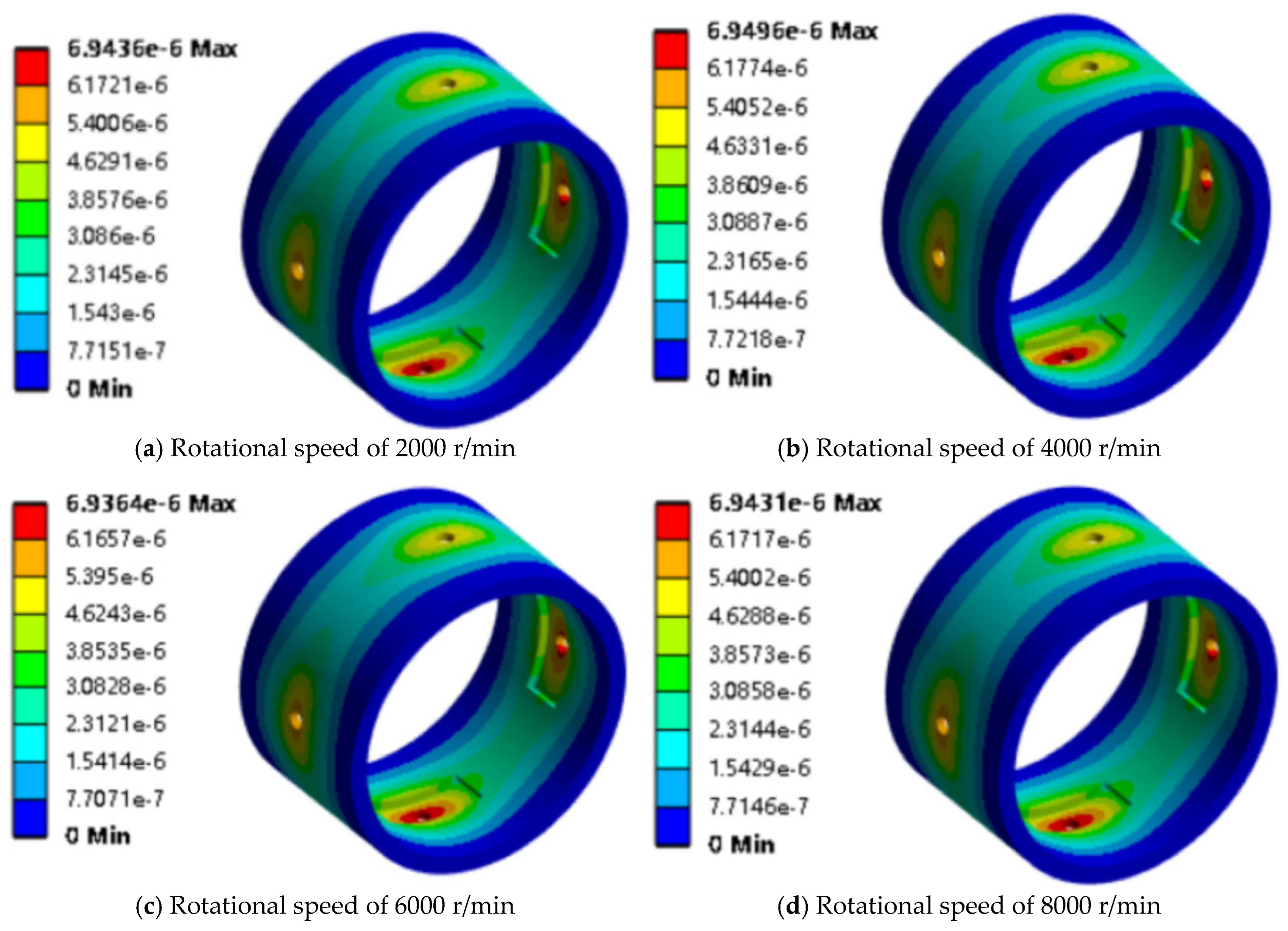
1. Introduction

As the demand for high-performance rotating machinery increases in manufacturing, equipment speeds and load capacities continue to rise. This is especially true in fields like automotive and aerospace, where the performance requirements for rotating components are becoming more stringent. Bearings, as key components supporting rotating shafts, play a critical role. The lubrication performance of bearings directly affects the operating efficiency and lifespan of the equipment. In recent years, S-CO₂ has attracted significant attention due to its excellent physical properties and potential economic advantages. In its supercritical state, S-CO₂ has liquid-like high density and gas-like low viscosity. It also provides superior heat transfer performance and is cost-effective. These properties make it highly promising for use in high-speed and high-load mechanical systems. This study uses a four-oil-chamber S-CO₂ hydrodynamic bearing as the research model. The goal is to analyze its lubrication performance under dynamic conditions.

Conventional bearings often use standard lubricants. However, the four-pocket S-CO₂ bearing has a structure designed for supercritical working conditions. It features four oil chambers arranged symmetrically, which provide stable and adjustable hydrodynamic support. These chambers help control local pressure based on load changes. This design increases the bearing’s ability to handle eccentric loads and improves system stability. Research on S-CO₂ hydrodynamic lubrication is ongoing. More studies are focusing on its performance under high-speed conditions. These efforts offer new directions for developing high-efficiency, high-speed bearing systems.

O. Reynolds proposed the slot-restriction hypothesis. This assumption simplified the fundamental equations of fluid dynamics. It laid the foundation for the development of thin film lubrication theory. Under this theoretical framework, the design, performance optimization, and stability of hydrodynamic bearings became key research topics. Liang et al. [1] proposed a deterministic mixed lubrication model. They analyzed the effects of surface roughness and elastic support on the performance of water-lubricated thrust bearings. Their work provides a modeling approach for multilayer soft material lubrication. Kocman et al. [2] evaluated four commonly used optimization algorithms for hydrodynamic lubrication problems. The results showed that the PSWM algorithm is the preferred option due to its stability and ease of use. To improve bearing stability under unsteady loads, Marinković et al. [3] combined theoretical modeling with experimental validation. Their results demonstrated improved stability and reduced friction under optimized lubrication states. Wang et al. [4] designed pressure relief grooves in the bearing structure. This significantly improved the lubricant film thickness and wear resistance. Usov et al. [5] used the finite element method to study elastic deformation in finite-length bearings. They found that under strong deformation, the minimum film thickness often occurs near the ends of the bearing. Chen et al. [6] used a nonlinear dynamic coefficient modeling approach. They combined simulation and experimental validation. They clarified the relationship between oil-film instability and rotor response. This work provides theoretical support for fault monitoring and prediction. To understand the impact of cavitation, Wettmarshausen et al. [7] introduced a non-condensable gas model. They proposed the pseudocavitation theory. Their simulation results agreed closely with experiments. Furthermore, Stefani et al. [8] observed coupled lateral and torsional vibrations under periodic excitation. They proposed a new method to determine stability thresholds using Hopf bifurcation theory. Yu et al. [9] analyzed the effect of speed variation on film stability in dual-chamber hydrostatic bearings. Their experiments confirmed the evolution of dynamic disturbance response and stiffness coefficients. Hong et al. [10] addressed offset-load impact issues. They introduced flexible groove structures at the bearing ends. This design reduced impact loads effectively. It enhanced film stability and bearing reliability.

With the progress of carbon neutrality strategies, the S-CO₂ Brayton cycle has gained attention due to its high efficiency and low emissions [11]. It is gradually becoming a core technology in next-generation energy systems. This trend brings new demands on the thermal stability and structural adaptability of lubrication systems. Li et al. [11] compared different working fluids. They pointed out that using CO₂ as a lubricant can significantly increase the static load capacity of bearings. This effect is especially noticeable under small film thickness conditions. Bi et al. [12] developed a thermal equilibrium model for high-speed tilting pad bearings. They found that thermo-compressibility has a much greater impact on static and dynamic performance than viscosity. They also noted a strong dependence on rotational speed. To meet the challenges of high pressure and high temperature in S-CO₂ systems, Mehdi et al. [13] proposed a simulation method for externally pressurized tilting pad bearings using real-gas modeling. They showed that mixed lubrication greatly improves film thickness and stiffness. They also developed a four-oil-chamber model suitable for high-speed ranges from 60,000 to 100,000 rpm. Yi et al. [14] studied the static and dynamic characteristics of supercritical CO₂ tilting pad bearings. They proposed a new thermo-elastohydrodynamic mixed lubrication model that considers thermal-mechanical coupling. Zhu et al. [15] conducted experiments to measure dynamic stiffness and damping responses. They tested the bearing under high-frequency excitation and low-load conditions. Their results provide design parameters for the hydrostatic start-up stage. Han et al. [16] used the perturbation derivative method to calculate frequency-dependent dynamic coefficients of S-CO₂ foil bearings. They found that, when structural flexibility is considered, the Reynolds number better describes system response than the traditional bearing number. Zhang et al. [17] applied an artificial neural network algorithm. The method effectively improved flow regime prediction accuracy and helped overcome modeling inaccuracy in the transitional flow region.

In the field of thermal–fluid coupling, Wang et al. [18] conducted experiments under high heat flux and low flow rate. They found that buoyancy and sharp changes in thermophysical properties are the main causes of heat transfer deterioration in S-CO₂. This mechanism may also affect bearing oil films, especially in regions prone to cavitation. Fang et al. [19] developed an oil-free lubrication pump. It successfully operated at 8100 r/min. This result confirms the system integration advantages of using S-CO₂ as the working medium. Colgan et al. [20] performed hydrodynamic bearing experiments. They showed that an S-CO₂ lubrication system can operate stably at 7.336 MPa. No abnormal whirl was observed in the bearing. This supports the potential of S-CO₂ in simplifying sealing system design. In the thrust bearing field, Patel et al. [21,22] used 3D CFD analysis to develop a hybrid structure model and a four-orifice hydrostatic model. They studied how nozzle arrangement and clearance design influence load capacity and stiffness. Niu et al. [23] conducted a study on S-CO₂ lubricated four-oil-cavity hydrodynamic journal bearings, focusing on the impact of oil cavity geometry and inlet parameters on load capacity and deformation.

Although many studies have analyzed the structural parameters of S-CO₂ lubricated bearings, their scope is still limited. Most existing work focuses on hydrostatic lubrication structures. Many studies also only consider a narrow range of operating conditions. In particular, Reference [23] mainly discusses the effects of oil cavity geometry and inlet conditions. It examines how these factors influence load capacity and structural deformation. However, it does not study ultra-high-speed operating conditions. It does not analyze the evolution of oil film pressure distribution. It also does not investigate the enlargement of negative pressure regions. As a result, the cavitation risk under high-speed conditions is not clearly evaluated.

In comparison, research on supercritical carbon dioxide-lubricated bearings is still limited. Existing studies mainly focus on modeling and experimental validation of hydrostatic lubrication designs. Under ultra-high-speed operating conditions, studies on the frictional dynamic response of S-CO₂ hydrodynamic or mixed-lubrication bearings remain scarce. There is still a lack of systematic evaluations on how geometric parameters and operating variables affect their hydrodynamic performance.

To address the above limitations, this study applies a fluid–structure interaction method. The ANSYS Workbench 2024 R1 platform is used to combine computational fluid dynamics with structural mechanics analysis. Numerical simulations are carried out to study the lubrication behavior of a four-chamber S-CO₂ hydrodynamic sliding bearing under ultra-high-speed conditions. The research includes an analysis of rotational speed effects under multiple parameter conditions. It also examines the influence of cavitation on bearing performance within a specific speed range. The innovations of this work are as follows:

(1)

Real-gas thermophysical parameters are incorporated into the hydrodynamic lubrication model. The temperature- and pressure-dependent properties of S-CO₂ are included to improve the physical accuracy of numerical predictions.

(2)

A systematic coupled analysis of speed, geometric design parameters, and cavitation effects is conducted in the ultra-high-speed range. The study reveals their combined influence on maximum oil film pressure, load capacity, and friction coefficient.

(3)

Based on the analysis, several optimization insights for S-CO₂ lubricated bearings in high-speed rotating machinery are obtained. These findings provide theoretical guidance and design implications for the engineering application of new lubrication systems.

2. Governing Equations

2.1. Thermophysical Property Equations of S-CO₂

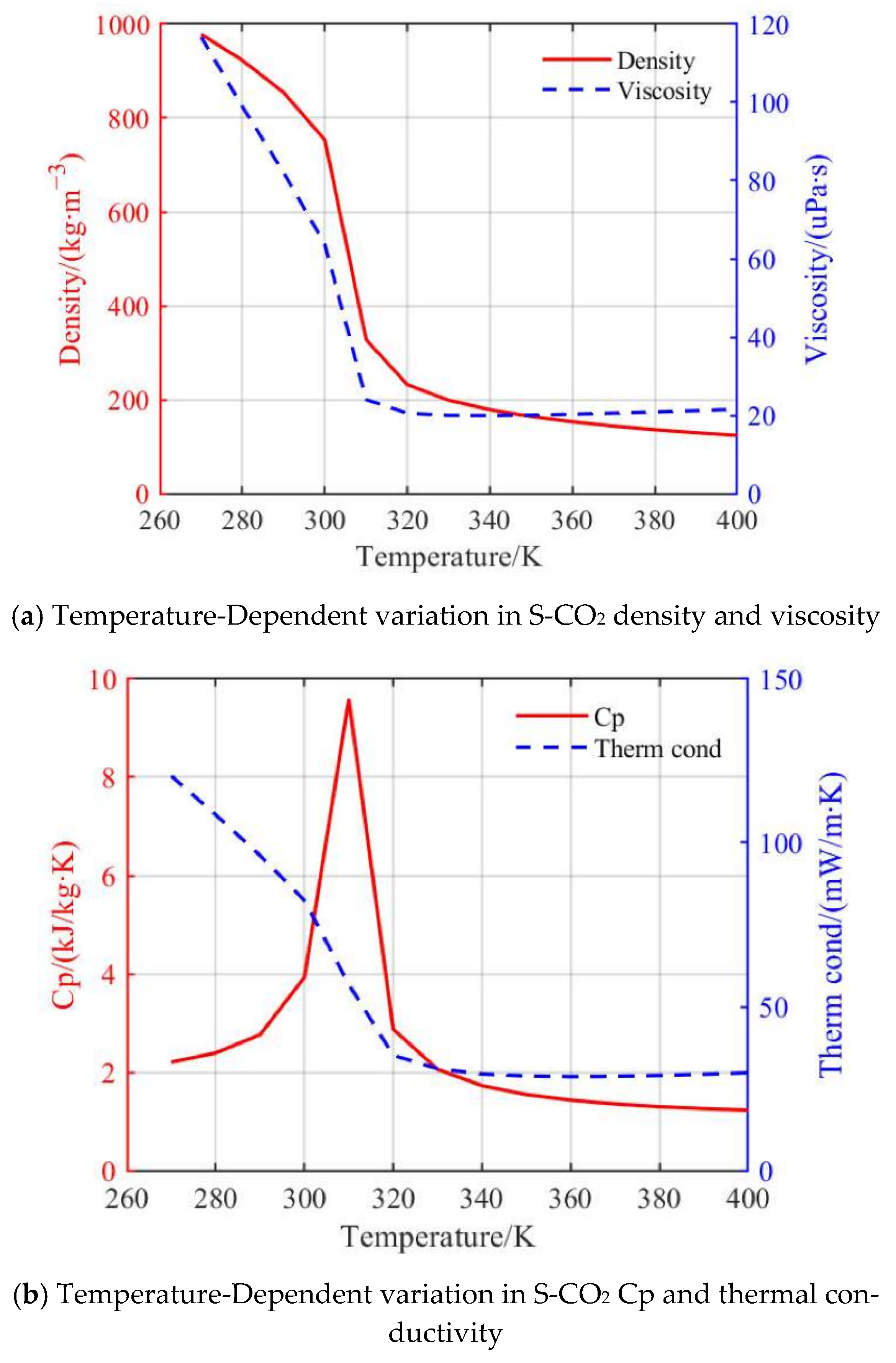
Figure 1 illustrates how S-CO₂ exhibits complex thermophysical changes when approaching its critical state. At a working pressure of 8 MPa, the specific heat capacity shows a distinct peak near the critical point before transitioning into a more stable range. Meanwhile, the material properties such as density and thermal conductivity experience an abrupt reduction once the fluid crosses this critical threshold. The dynamic viscosity of S-CO₂ also reflects unique dual-phase behavior; it behaves like a liquid under certain conditions and like a gas in others. Notably, at the critical point, its viscosity sharply decreases to nearly 2.5 × 10⁻⁵ Pa·s, which is far below the typical viscosity observed in standard CO₂. Furthermore, in the supercritical phase, S-CO₂ maintains a relatively stable state, and its inherently low viscosity contributes to minimizing frictional energy losses when used in hydrodynamic journal bearings.

In practical engineering applications, thermophysical data of fluids like CO₂ are typically accessed from professional databases instead of manual calculations. This study utilized the NIST REFPROP 10.0 software to retrieve accurate physical property values. The critical temperature and pressure for carbon dioxide were defined as 304.1 K and 7.37 MPa, respectively. These parameters were applied to ensure the reliability of density and viscosity data in all simulations. Initially, pure CO₂ was selected in the simulation’s Fluids module, where its thermodynamic state was specified using the above critical constants. Relevant calculation models were applied to extract property data, allowing the relationships between temperature, pressure, and properties like viscosity and density to be visualized through plotted curves. High-precision data tables were generated accordingly.

Subsequently, these property datasets were imported into MATLAB R2022b. Using curve-fitting techniques, explicit mathematical expressions for density and viscosity variations were established. These fitted equations were then embedded into Fluent, enabling dynamic property adjustments during simulations of supercritical CO₂ flow under varying operational conditions. This combined method leveraged REFPROP’s data precision and MATLAB’s equation modeling to achieve accurate and stable simulation outcomes.

2.2. Basic Governing Equations of CFD

In this part, the simulation approach for turbulent flow inside a four-pocket hydrodynamic journal bearing is described. The CFD module was used to carry out the flow analysis. Two primary equations were selected to define the fluid motion: the continuity equation and the momentum equation. These equations are essential to ensure an accurate prediction of the flow behavior. Their vector expressions are listed below.

The fluid continuity equation remains as:

$${\displaystyle \frac{\partial \rho }{\partial t}}+\nabla (\rho \cdot \overrightarrow{v})=0$$

(1)

In the equation, $\rho$ represents the fluid density; t is time; ν is the velocity vector.

The momentum conservation equation:

$$\begin{array}{c}{\displaystyle \frac{\partial \left(\rho \mathrm{u}\right)}{\partial t}}+\nabla \cdot (\rho uV)=-{\displaystyle \frac{\partial p}{\partial x}}+{\displaystyle \frac{\partial {\tau }_{xx}}{\partial x}}+{\displaystyle \frac{\partial {\tau }_{yx}}{\partial y}}+{\displaystyle \frac{\partial {\tau }_{xx}}{\partial z}}+\rho f_x\\ \\ {\displaystyle \frac{\partial \left(\rho v\right)}{\partial t}}+\nabla \cdot (\rho vV)=-{\displaystyle \frac{\partial p}{\partial y}}+{\displaystyle \frac{\partial {\tau }_{xy}}{\partial x}}+{\displaystyle \frac{\partial {\tau }_{yy}}{\partial y}}+{\displaystyle \frac{\partial {\tau }_{yz}}{\partial z}}+\rho f_y\\ \\ {\displaystyle \frac{\partial \left(\rho w\right)}{\partial t}}+\nabla \cdot (\rho wV)=-{\displaystyle \frac{\partial p}{\partial z}}+{\displaystyle \frac{\partial {\tau }_{xz}}{\partial x}}+{\displaystyle \frac{\partial {\tau }_{yz}}{\partial y}}+{\displaystyle \frac{\partial {\tau }_{zz}}{\partial z}}+\rho f_z\\ \end{array}$$

(2)

In Equation (1): $\rho$ is the density of the lubricant, $V$ is the velocity vector, $u, v, w$ is the velocity component of the lubricant along the $x, y, z$ axis, ${\tau }_{xx}, {\tau }_{xy}, {\tau }_{xz}$ represents the shear force components, $f_x, f_y, f_z$ is the body force acting on the lubricant as it moves along the $x, y, z$ axis.

The Navier–Stokes equation is given as:

$$\rho {\displaystyle \frac{\mathrm{D}\mathrm{V}}{\mathrm{D}\mathrm{t}}}=-\nabla \mathrm{p}+\mu {\nabla }^2\mathrm{V}+{\displaystyle \frac{\mu }{3}}\nabla \left(\nabla \cdot \mathrm{V}\right)$$

(3)

Here, $\rho$ and $\mu$ represent the density and dynamic viscosity of the lubricant, respectively. $\mathrm{V}$ is the velocity vector of the lubricant, and $\mathrm{p}$ stands for the fluid pressure.

The Fluent solver provides several turbulence models to simulate different flow conditions. Among them, the standard k–ε model is widely used for fully developed turbulence. It is suitable for simulating lubrication conditions with high Reynolds numbers.

The transport equation for the turbulent kinetic energy (k) is expressed as:

$$\rho {\displaystyle \frac{\mathrm{d}\mathrm{k}}{\mathrm{d}\mathrm{t}}}={\displaystyle \frac{\partial }{\partial {\mathrm{x}}_{\mathrm{i}}}}\left[\left(\mu +{\displaystyle \frac{{\mu }_{\mathrm{t}}}{{\sigma }_{\mathrm{k}}}}\right){\displaystyle \frac{\partial \mathrm{k}}{\partial {\mathrm{x}}_{\mathrm{i}}}}\right]+{\mathrm{G}}_{\mathrm{b}}+{\mathrm{G}}_{\mathrm{k}}-\rho \epsilon -{\mathrm{Y}}_{\mathrm{M}}$$

(4)

The transport equation for the turbulence dissipation rate (ε) is given as:

$$\rho {\displaystyle \frac{\mathrm{d}\epsilon }{\mathrm{d}\mathrm{t}}}={\displaystyle \frac{\partial }{\partial {\mathrm{x}}_{\mathrm{i}}}}\left[\left(\mu +{\displaystyle \frac{{\mu }_{\mathrm{t}}}{{\sigma }_{\mathrm{k}}}}\right){\displaystyle \frac{\partial \epsilon }{\partial {\mathrm{x}}_{\mathrm{i}}}}\right]+{\mathrm{C}}_{1\epsilon }{\displaystyle \frac{\epsilon }{\mathrm{k}}}\left({\mathrm{G}}_{\mathrm{k}}+{\mathrm{C}}_{3\epsilon }{\mathrm{G}}_{\mathrm{b}}\right)-{\mathrm{C}}_{2\mathrm{t}}\rho {\displaystyle \frac{{\epsilon }^2}{\mathrm{k}}}$$

(5)

In the above equations the turbulent viscosity is defined as ${\mu }_t=\rho C_{\mu }{\displaystyle \frac{K^2}{\epsilon }}$, $G_k$ denotes the generation of turbulent kinetic energy due to velocity gradients, $Y_{M }$ represents the contribution of fluctuating dilatation to the overall dissipation rate and $G_b$ accounts for the generation of turbulence induced by buoyancy effects. $C_{1\epsilon }=1.44;{ C}_{2k}=1.92;{ C}_{3k}=0.09;{ C}_{\mu }=0.09; {\sigma }_k=1.0; {\sigma }_k=1.3.$

In this research, the lubrication analysis of the S-CO₂ hydrodynamic bearing adopts several basic premises. Firstly, it is presumed that turbulence occurs within the narrow gap between the shaft and the bearing surface. Secondly, due to the minimal viscosity of S-CO₂, the frictional heating effect generated in the gas layer is considered insignificant, allowing the flow to be treated under constant temperature conditions. Thirdly, it is assumed that gas molecules stick perfectly to both the journal and bearing surfaces, resulting in no slip condition at the interface. Lastly, forces arising from fluid inertia and external fields, such as gravity, are disregarded in the simulation to simplify the model.

Based on the above assumptions, Equations (1)–(5) were applied under actual boundary conditions. This yields the general form of the Reynolds equation for oil film bearing analysis, expressed as Equation (6):

$$\begin{array}{ll}& \{\begin{array}{c}{\displaystyle \frac{{\partial }^{2}u}{\partial y^2}}={\displaystyle \frac{1}{\mu }}{\displaystyle \frac{\partial p}{\partial x}}\\ {\displaystyle \frac{{\partial }^{2}w}{\partial y^2}}={\displaystyle \frac{1}{\mu }}{\displaystyle \frac{\partial p}{\partial z}}\\ {\displaystyle \frac{\partial p}{\partial y}}=0\end{array}\\ & {\displaystyle \frac{\partial }{\partial x}}\left({\displaystyle \frac{\rho h^3}{\eta }}{\displaystyle \frac{\partial \rho }{\partial x}}\right)+{\displaystyle \frac{\partial }{\partial z}}\left({\displaystyle \frac{\rho h^3}{\eta }}{\displaystyle \frac{\partial \rho }{\partial z}}\right)=6\left(V_1-V_2\right){\displaystyle \frac{\partial \left(\rho h\right)}{\partial x}}+12\rho {\displaystyle \frac{ \mathrm{d}h}{ \mathrm{d}t}}\\ & \end{array}$$

(6)

When the bearing is in a static condition, the lubricant film thickness remains constant. The equation can be further simplified:

$${\displaystyle \frac{\partial }{\partial x}}\left({\displaystyle \frac{h^3}{\eta }}{\displaystyle \frac{\partial p}{\partial x}}\right)+{\displaystyle \frac{\partial }{\partial z}}\left({\displaystyle \frac{h^3}{\eta }}{\displaystyle \frac{\partial p}{\partial y}}\right)=6V\eta {\displaystyle \frac{ \mathrm{d}h}{ \mathrm{d}x}}$$

(7)

Given these conditions, the equation for the local Reynolds number is established. Additionally, the governing equation for compressible turbulent flow, expressed in dimensionless form under steady operation, is formulated. These are derived from fundamental principles, using both the Navier–Stokes and continuity equations as the basis. To account for turbulence effects more accurately, a specific correction coefficient is applied to the model.

$$\mathrm{R}\mathrm{e}=\rho \Omega \mathrm{R}\mathrm{h}/\mu$$

(8)

$${\displaystyle \frac{\partial }{\partial \phi }}\left({\displaystyle \frac{12}{{\mathrm{K}}_{\mathrm{x}}}}{\displaystyle \frac{{\mathrm{h}}^3\stackrel{\mathrm{‾}}{\rho }}{\stackrel{\mathrm{‾}}{\mu }}}{\displaystyle \frac{\partial \stackrel{\mathrm{‾}}{\mathrm{p}}}{\partial \theta }}\right)+{\left({\displaystyle \frac{\mathrm{D}}{\mathrm{L}}}\right)}^2{\displaystyle \frac{\partial }{\partial \lambda }}\left({\displaystyle \frac{12}{{\mathrm{K}}_{\mathrm{z}}}}{\displaystyle \frac{{\mathrm{h}}^3\stackrel{\mathrm{‾}}{\rho }}{\stackrel{\mathrm{‾}}{\mu }}}{\displaystyle \frac{\partial \stackrel{\mathrm{‾}}{\mathrm{p}}}{\partial \lambda }}\right)=\Lambda {\displaystyle \frac{\partial \rho \mathrm{h}}{\partial \theta }}$$

(9)

In this context, the bearing geometry and gas film parameters are defined as follows. The symbols λ and φ denote the axial and circumferential positions on the bearing surface. The parameter c indicates the radial clearance between the shaft and bearing, while h refers to the thickness of the gas film within the lubricating layer. ${\mu }_a$ and ${\rho }_a$ are the viscosity (Pa·s) of CO₂ and ambient density (kg/m³). Additionally, ${ p}_a$ stands for the atmospheric pressure surrounding the bearing, given in pascals (Pa). The notation “Λ” is used to symbolize the bearing number in the equations.

Reference [24] has explored various turbulence models to assess their performance in lubrication flow simulations. Among these, the standard k–ε model demonstrated good stability and computational efficiency, especially when dealing with turbulent flows at high Reynolds numbers. The study also analyzed the RNG k–ε model, which adapts better to flow regions with large strain rates, and the Reynolds Stress Model (RSM), known for its ability to represent anisotropic turbulence structures more precisely. However, RSM tends to be less reliable in multiphase flow simulations due to noticeable calculation errors. Additionally, it is known that the standard k–ε model’s prediction capability weakens in situations involving complex flow patterns, such as strong convective effects or when the Reynolds number is low, often resulting in an underestimation of recirculation areas. In the present work, the flow environment does not exhibit intense convection, and the Reynolds number remains sufficiently high. Therefore, the standard k–ε model was selected for solving the governing equations, balancing accuracy with computational cost and solution stability.

2.3. Fluid–Structure Interaction

In fluid–structure interaction, the fluid forces calculated by Computational Fluid Dynamics interact with the deformation of the bearing housing computed by structural analysis. FSI can be classified into one-way and two-way coupling. In one-way FSI, the pressure distribution obtained from the CFD simulation is transferred to the solid domain. This allows the calculation of deformation and load distribution of the bearing housing. In this approach, the fluid domain is not updated after deformation. It is suitable for applications where structural deformation is small and does not significantly affect the flow field. This type of coupling is also referred to as weak coupling. In two-way FSI, the pressure distribution in the fluid domain interacts with the structure. Structural deformation, in turn, changes the flow characteristics of the fluid domain. This method is used when large structural deformation significantly alters the fluid flow. In this study, a one-way FSI method is used. The bearing deformation is small, so there is no need to reconstruct the flow field. The workflow of the one-way FSI approach is shown in Figure 2.

3. Computational Model and Simulation Conditions

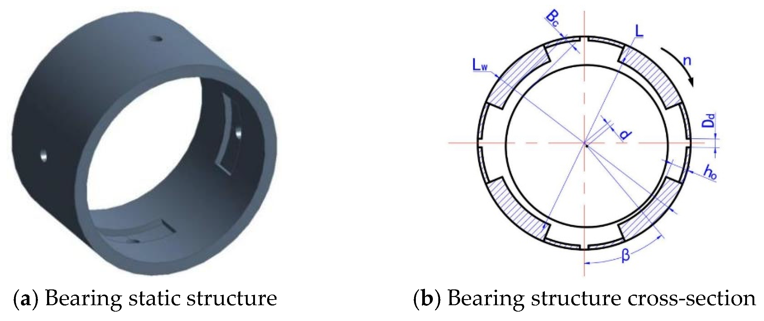
This study focuses on a well-established radial journal bearing that incorporates four lubrication pockets. These pockets are symmetrically positioned around the bearing circumference, with each one connected to its corresponding inlet port. Inside the lubrication film area, cavities of equal size are designed to ensure smooth storage and continuous supply of the working fluid. Detailed geometric dimensions of the bearing are summarized in

Table 1. Geometric and operational specifications of the journal bearing.

Item	Value
Bearing inner diameter L (mm)	30
Bearing length B (mm)	20
Depth of the oil groove ho (mm)	2
Width of the oil groove Bo (mm)	5
The number of oil grooves	4
Eccentric angle (rad)	49.8
Diameter of oil holes Dd (mm)	2
Bearing outer diameter Lw (mm)	34
Radial clearance (mm)	0.08
Eccentricity ratio	0.1
Oil supply pressure po (MPa)	8
Rotating speed n (r/min)	2000–20,000

. For the 3D modeling process, the oil film region was developed using the Design Modeler tool. This provided a clear representation of the bearing’s structural configuration, which is illustrated in Figure 3. The constructed simulation domain reflects both the internal flow path and external boundaries necessary for the hydrodynamic analysis.

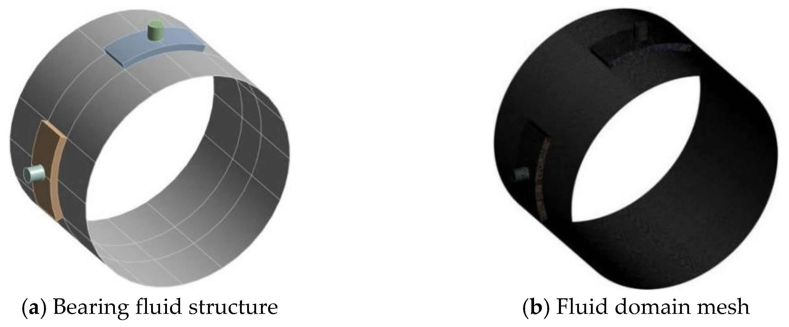
Due to the presence of a thin lubricant film, mesh instability could arise during simulation. To prevent this, the fluid domain was segmented into several distinct zones, as depicted in Figure 4a. The sweep meshing method was specifically used in the areas where the lubricant comes into direct contact with the bearing surfaces. In total, the mesh was partitioned into 140 regions, including 25 internal layered grids. Finer mesh elements were applied in the cavitation-prone regions, increasing the total number of cells to 200. Local mesh density was also increased at the inlets, outlets, and regions where sharp velocity changes occur. Element sizes were controlled within strict limits. The smallest mesh element measured 1 × 10⁻⁶ m, while the largest was set to 4 × 10⁻⁵ m. For curved surfaces, a minimum curvature element size of 2 × 10⁻⁷ m was defined. The mesh quality achieved a value of 0.9, which is sufficient to ensure reliable computational accuracy and numerical convergence. Figure 4b presents the overall mesh distribution.

In FLUENT, 50 solver threads were utilized to improve the efficiency of steady-state simulations. The cavitation phenomena were modeled using the Schnerr–Sauer approach within the mixture model framework. A pressure-based coupled solver was applied to handle fluid–structure interactions with better numerical stability. First-order discretization schemes were adopted during computation. The convergence criterion was set so that all residuals had to fall below 1 × 10⁻⁴. Boundary conditions were then applied according to the operational setup of the bearing system. The boundary conditions were set as follows:

(1)

The inner surface of the bearing was set as a rotating wall, while the outer surface remained stationary. All four inlet ports were defined as pressure inlets with a specified pressure of 8 MPa. Both ends of the bearing were configured as pressure outlets, set to atmospheric conditions.

(2)

A constant temperature of 320 K was applied to the inlet and outlet surfaces, the rotating inner wall, and the fixed outer wall. The fluid properties of CO₂ were calculated using the REFPROP-based real-gas model to capture its non-linear thermophysical behavior.

(3)

Considering the high Reynolds number of the flow, the standard k–ε turbulence model was adopted for turbulence closure. The SIMPLEC algorithm was employed to handle the momentum equations efficiently. The simulation ensured that pressure distribution followed hydrodynamic lubrication principles, with the inlet pressure set at the supercritical CO₂ critical point to maintain internal pressurization.

4. The Grid Independence Verification and Model Validation

To maintain numerical accuracy despite the narrow radial gap of the lubricant film, a mesh sensitivity study was essential. This step ensures that mesh refinement does not cause unnecessary increases in computational effort while still keeping discretization errors within acceptable limits. The simulation began with predefined initial parameters to maintain consistency across all cases as follows: Eccentricity ratio of 0.1, Radial clearance of 0.08 mm, Inlet diameter of 2 mm, Oil pocket geometry with an axial width of 5 mm and a chamber arc angle of 45 degrees. Mesh sizes with 1,500,000, 1,750,000, 2,000,000, 2,250,000, 2,500,000, and 2,750,000 million cells were tested. Details are shown in

Table 2. Target values for different mesh quantities.

Mesh Number	Maximum Pressure (Mpa)	Minimum Pressure (Kpa)	Load Capacity (N)	Friction Coefficient
1,500,000	10.6	72.3	43.613	0.20012
1,750,000	10.8	10.5	39.600	0.13998
2,000,000	11.0	−42.7	31.092	0.12672
2,250,000	11.0	−38.2	29.729	0.11530
2,500,000	10.8	−41.6	29.123	0.11582

and Figure 5.

Bearing capacity was used as the indicator for error analysis. An error within 5% is generally considered to indicate mesh independence. The verification results showed the following differences in bearing capacity between adjacent mesh sizes: 9.2% between 1,500,000 and 1,750,000 cells, 21.5% between 1,750,000 and 2,000,000 cells, 6.2% between 2,000,000 and 2,250,000 cells, 2.2% between 2,250,000 and 2,500,000 cells, and less than 2.2% between 2,500,000 and 2,750,000 million cells. When the number of mesh elements exceeds 2,000,000, the change in oil film load-carrying capacity becomes negligible. Considering the balance between accuracy and computational cost, a mesh size of 2,000,000 elements was selected for this study.

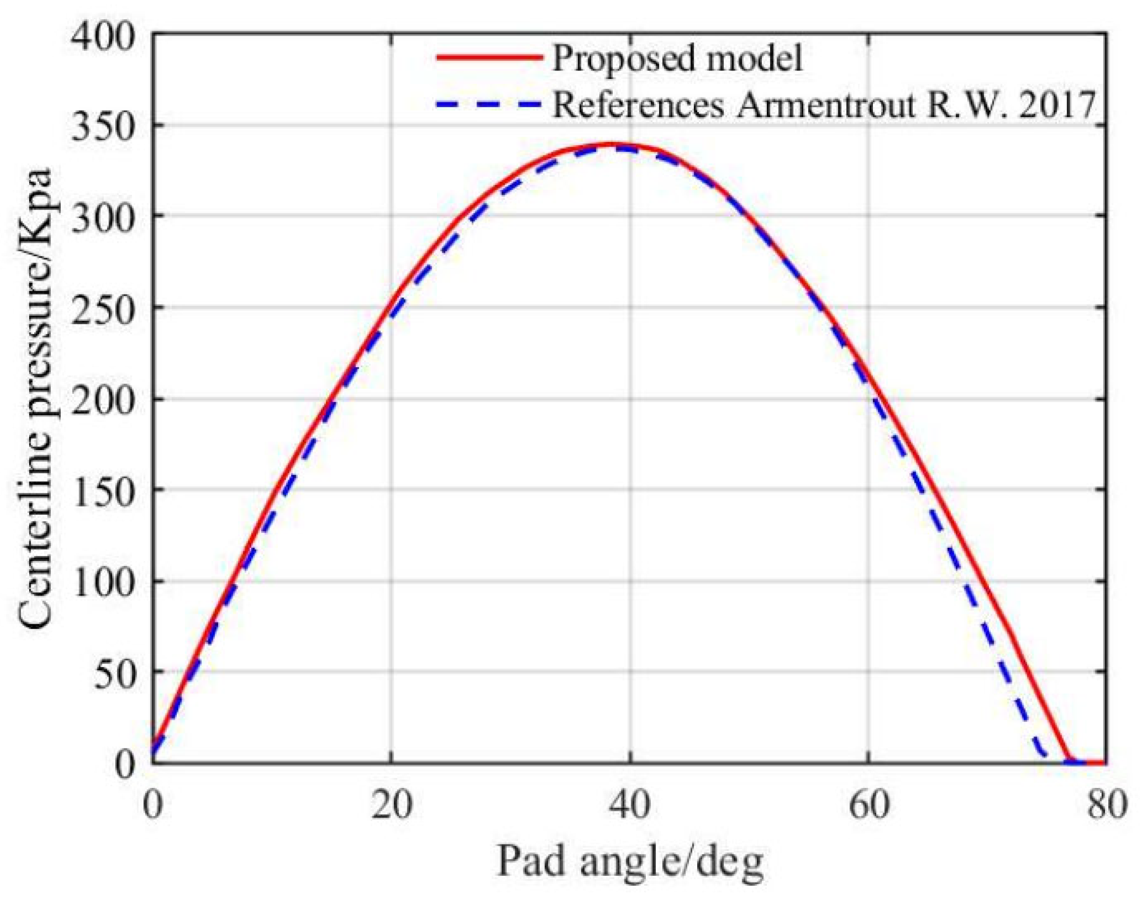
To evaluate the credibility of the computational approach, a benchmark comparison was performed using a water-lubricated tilting-pad bearing model documented in Reference [25]. For consistency, the same mesh setup and boundary configurations from the literature were applied here. A case study was conducted for a pad with a 72° installation angle. See Figure 6 for details. The observed difference in peak pressure between the two models was 5.7%. This minor variation primarily resulted from the difference in turbulence models applied; the current study adopted a k–ε turbulence approach, which performs well in high-Reynolds-number scenarios, while the reference employed a Navier–Stokes solver better suited for low-speed flows. Both analyses neglected inertia forces. Despite these differences, the overall pressure contour matched well, confirming that the present computational model is valid for the intended simulation conditions. Since publicly available experimental data for S-CO₂ lubricated bearings are still very limited, a well-documented water-lubricated bearing model reported in the literature was preferentially used for method validation in this study. It should be emphasized that this validation is intended to verify the numerical approach, solution procedure, and pressure distribution behavior, rather than to establish complete physical equivalence of working conditions. In addition, the mesh independence analysis and convergence criteria used in this work are consistent with those reported in existing S-CO₂ bearing studies. The pressure evolution characteristics and load-carrying trends obtained in this study also show good agreement with previously published S-CO₂ lubrication results.

5. Results and Discussion

With the computational setup fixed and boundary conditions maintained, this research primarily explored how changes in rotational speed impact several key performance indicators. These include maximum oil film pressure, bearing deformation characteristics, load-bearing capacity, and friction coefficient under operational conditions. The following parameters were set 2000 r/min to 20,000 r/min.

Effect of Rotational Speed

When the inlet diameter is 2 mm, the eccentricity is 0.1, the radial clearance is 0.3 mm, and the oil pocket size (axial width × oil pocket angle) is 5 × 45, the oil film pressure distribution and bearing deformation regions at different speeds are shown in Figure 7 and Figure 8. (Clear color bar ranges and the evolution of key pressure regions are retained in the figures, which makes the results more intuitive. And the “8E3” is mean “8 × 10³”)

As shown in Figure 7, the oil film pressure distribution changes significantly with increasing rotational speed. The maximum positive pressure is mainly concentrated at the center of the bearing and near the upper and lower inlet ports. As the speed increases (Figure 7a–j), the positive pressure region becomes more concentrated and pronounced. Meanwhile, the negative pressure region gradually expands toward both sides of the inlets. Negative pressure becomes more significant, especially near the upper and lower inlet ports. The formation of the negative pressure zone is closely related to the hydrodynamic effects generated by high-speed rotation. As the speed increases (Figure 7e–j), the area of the negative pressure zone increases. The negative pressure becomes more concentrated on both sides of the inlet ports. It should be noted that the color bar in the figure provides the specific values of the maximum positive pressure and minimum negative pressure under different rotational speeds. Therefore, the figure not only shows the pressure distribution trend but also offers clear quantitative information.

As shown in Figure 8 and Figure 9, the bearing deformation region shifts with increasing rotational speed. The deformation tends to move from the bottom oil chamber toward the right side of the inlet region (Figure 8a–e). Between 10,000 r/min and 20,000 r/min, the amount of bearing deformation increases significantly. These changes indicate that increasing rotational speed not only enhances the oil film pressure but also intensifies the bearing deformation.

As shown in Figure 10 and Figure 11, both the maximum and minimum oil film pressures increase with rising rotational speed. When the speed ranges from 4000 r/min to 12,000 r/min, the positive pressure increases sharply from 10 MPa to 10.4 MPa. As a result, the hydrodynamic effect inside the bearing is enhanced, leading to higher oil film pressure. The minimum negative pressure also increases as the speed rises. At low speeds, the negative pressure region is small. As the speed increases, the negative pressure area gradually expands. At high speeds, this region becomes more pronounced, which may trigger cavitation. These results indicate that, under high-speed conditions, oil film stability is affected by the expansion of the negative pressure region. This may lead to instability of the lubrication film. Therefore, moderately reducing the rotational speed may help to mitigate cavitation effects.

Increasing the rotational speed generally enhances the load-carrying capacity of the oil film. At high speeds, the rising oil film pressure allows the bearing to support larger loads. The load capacity shows an increasing trend within a certain speed range. However, when the speed becomes too high, cavitation intensifies. This may cause the increase in load capacity to slow down or reach saturation. Between 2000 r/min and 20,000 r/min, the bearing deformation gradually increases. Especially near the inlet, the deformation zone clearly shifts toward the right side as speed increases. This indicates that the effect of rotational speed on bearing deformation cannot be ignored.

6. Conclusions

This study employed a fluid–structure interaction method to numerically analyze a four-pocket wedge hydrodynamic bearing lubricated by supercritical carbon dioxide under ultra-high-speed conditions. The pressure distribution of the lubricating gas film and the deformation profile of the bearing pad were obtained at different rotational speeds. This study revealed the relationships between bearing parameters and performance characteristics such as load capacity and friction coefficient. It also demonstrated the correlation and influence between rotational speed and cavitation effects.

• Oil film pressure increases significantly with rising rotational speed: As speed increases, both the maximum oil film pressure and load capacity show a nonlinear growth trend. Lubrication performance improves markedly at high speeds.
• Expansion of the negative pressure region leads to cavitation risk: Beyond a certain critical speed, strong negative pressure zones appear within the oil film. These zones are prone to cavitation, which weakens film stability and affects load capacity. The cavitation distribution obtained in this study mainly reflects the relative variation trend rather than an absolutely accurate prediction. This point should be taken into account when interpreting the results.
• Bearing deformation intensifies and shifts regionally with increasing speed: The deformation zone moves from the bottom toward the right side of the inlet. Comprehensive design of inlet size and eccentricity is needed to reduce structural stress concentration.
• Load capacity and friction coefficient increase with speed: Both parameters rise continuously as speed increases. However, at high speeds, the load capacity tends to plateau due to cavitation effects.
• The results show that increasing rotational speed in the high-speed range can effectively enhance the load-carrying capacity. However, it also intensifies negative pressure and structural deformation. Therefore, an engineering trade-off between load enhancement and operational stability is required in practical design. A reasonable operating speed range and structural parameters should be selected to avoid excessive negative pressure and potential instability risks.