
Dynamic Control of Coating Accumulation Model in Non-Stationary Environment Based on Visual Differential Feedback


Abstract
1. Introduction
- (1)
- Offline empirical adjustment method for spraying process parameters
- (2)
- Offline intelligent prediction of spraying process parameters
- Classic ANN optimization:
- Hybrid intelligent optimization algorithm:
2. Methods
2.1. Data Acquisition of Paint Spray Images Methodology
2.1.1. Principle of Conditional Equivalence for the Establishment of Datasets in Non-Stationary Environments
- (1)
- Rheological steady-state assumption: shear rate remains consistent in NT and NP;
- (2)
- Thermodynamic equilibrium assumption: paint temperature change rate ;
- (3)
- Pressure coupling separability: .
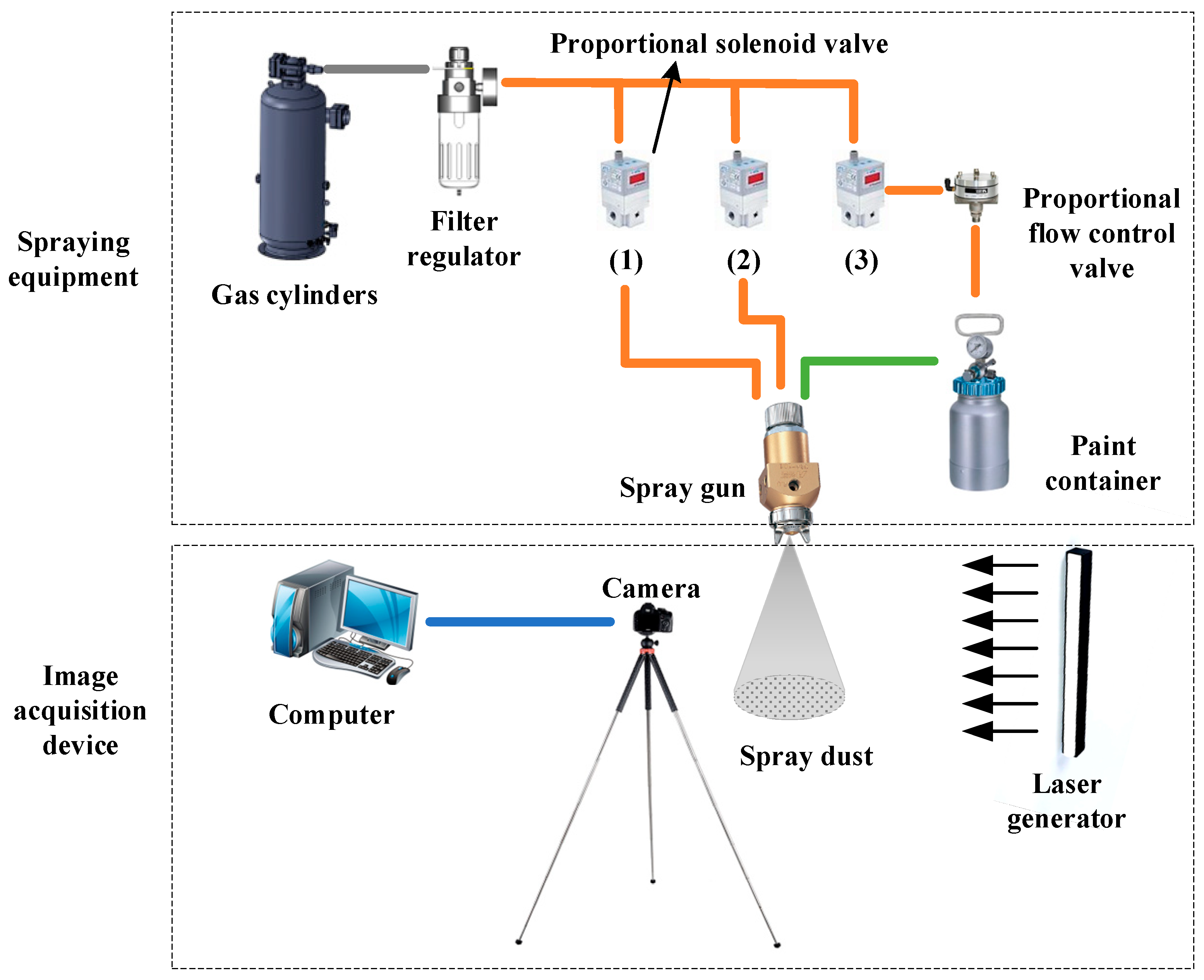
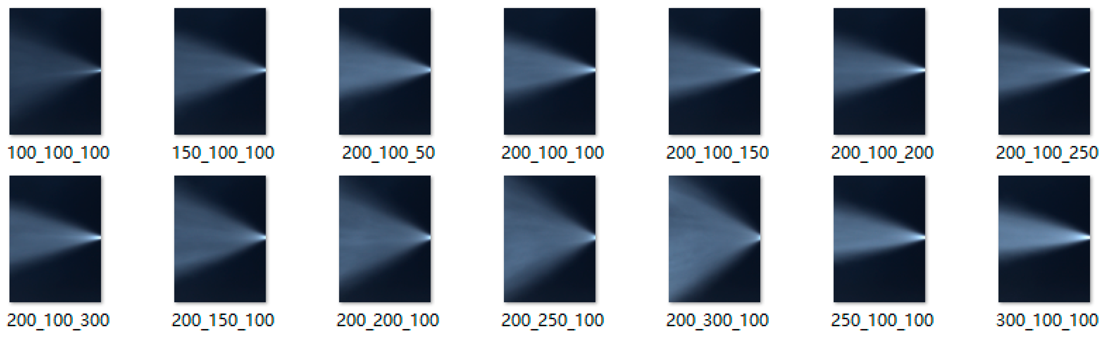
2.1.2. Data Acquisition Method of Paint Spray Image
- (1)
- Lock exposure parameters: Before starting the spray gun or during paint mist spraying, set and lock parameters such as shutter speed and aperture based on the background and paint mist brightness to prevent the camera from automatically adjusting exposure during the spraying process.
- (2)
- Fix white balance: In a stable lighting environment (before spraying or during paint mist spraying), set and lock the white balance value to prevent white balance drift caused by changes in paint mist color or ambient light.
- (3)
- Use industrial cameras with stable algorithms: Select industrial cameras with good interference resistance. Their internal image processing algorithms can better suppress fluctuations in exposure and white balance in dynamic scenes, maintaining image consistency.
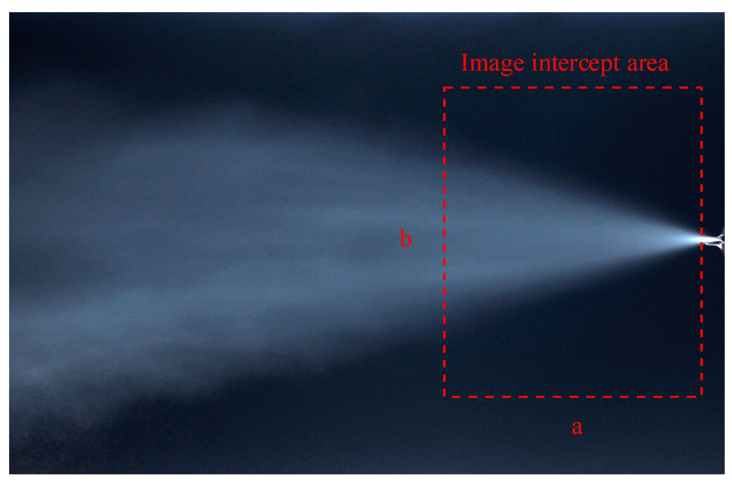
2.2. Image Data Processing and Labeling Methodology
- 1.
- Image cropping method
- (1)
- Selection criteria for cropping areas
- (2)
- Cropping operation specifications
- 2.
- Methods for labeling data
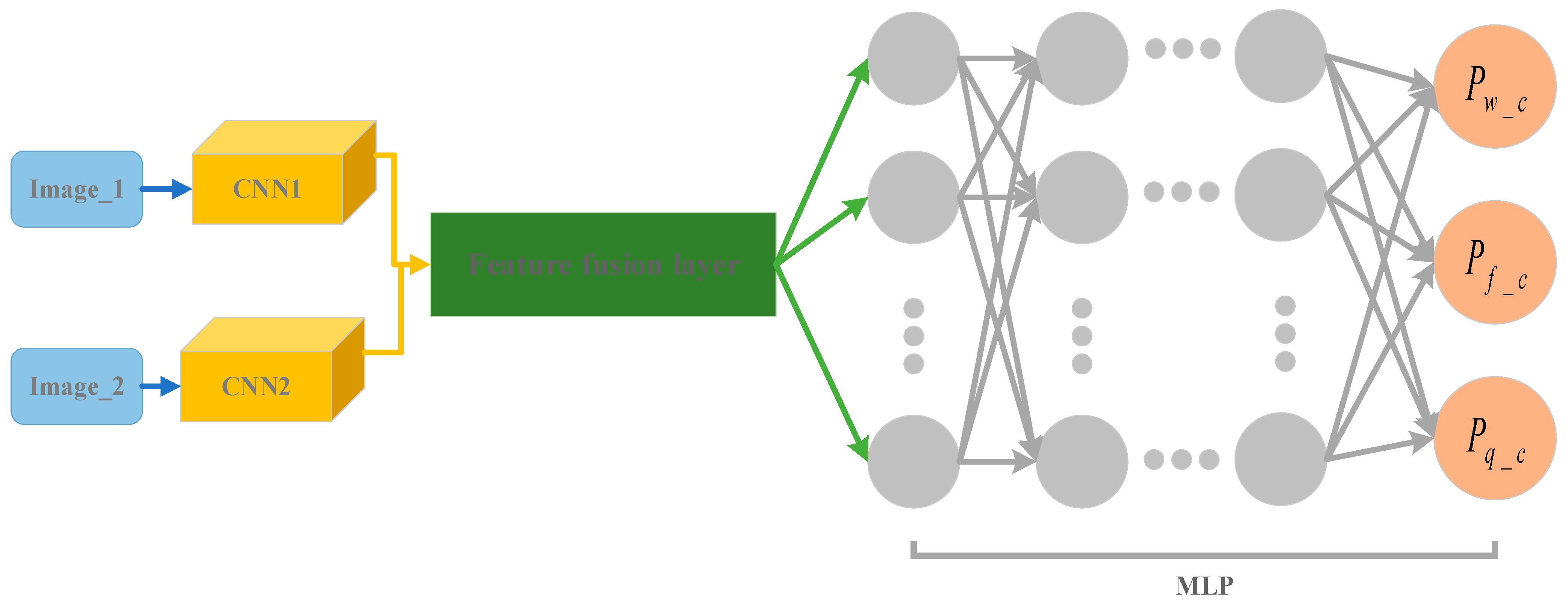
2.3. Image Difference Model Construction Methodology
2.3.1. Image Difference Modeling Architecture Design
2.3.2. Image Difference Model Optimization
- Adjusting the model architecture
- Increasing the model complexity, both by increasing the number of convolutional layers in the CNN or by using a larger convolutional kernel, in order to improve the feature extraction capability;
- Adjust the number of channels, which increases the number of filters in each layer of the CNN. You can start with a smaller number, such as 32 or 64, and gradually increase it to enhance feature expression capabilities.
- Increasing the number of hidden layer neurons in the MLP or adding more hidden layers.
- Optimization of the training process
- Adjusting the learning rate: In the initial stage, a relatively large learning rate is set to speed up the convergence of the model. If the loss function oscillates or does not converge during the training process, the learning rate may be too large, and then the learning rate is adjusted by exponential decay. By dynamically adjusting the learning rate, the model can converge quickly in the early stage of training, while maintaining a stable convergence state in the later stage, avoiding the overfitting problem caused by too large a learning rate.
- Adjusting the number of iterations: At the beginning, set a small number of iterations, and gradually increase the number of iterations by i times each time as the experiment proceeds. After each increase in the number of iterations, record the loss function value, accuracy, and other indicators of the model on the training set and validation set. When it is found that the performance of the model on the validation set is no longer improved, or even a downward trend, it indicates that the model may have been overfitted, and at this time, stop increasing the number of iterations, and select the number of iterations when the performance is optimal as the final number of training iterations.
- Regularization strategy: In order to prevent the model from overfitting, the dropout regularization technique is introduced into the model. Dropout improves the generalization ability of the model by randomly discarding a part of the neurons during the training process to reduce the co-adaptation phenomenon among neurons. At the same time, L2 regularization is applied to the weights of the model to limit the complexity of the model and prevent overfitting by adding the sum of squares of the weights as a penalty term in the loss function.
3. Experimental Method
3.1. Verification Test of the Principle of Equivalence of Conditions for Establishing Data Sets in Unstable Environments
3.2. Paint Mist Capture Device and Test
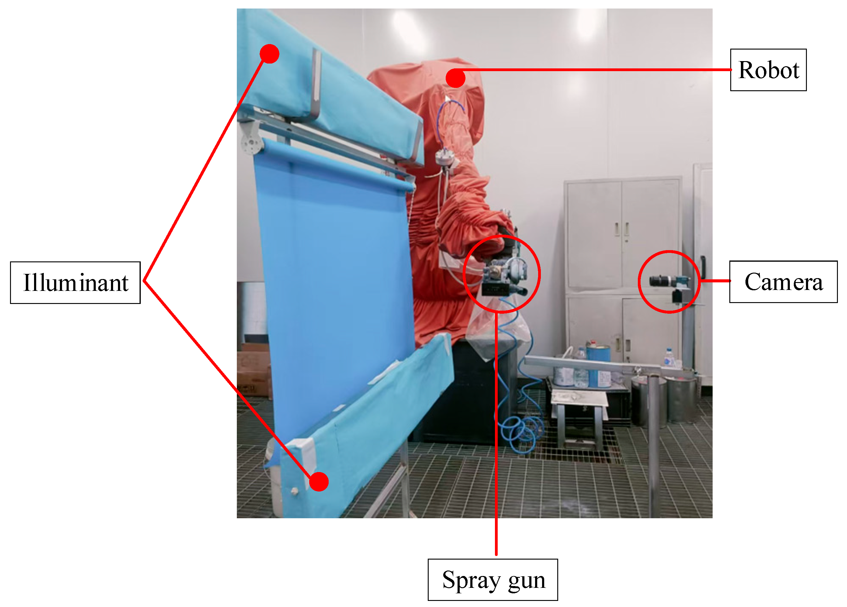
3.2.1. Experimental Setup
3.2.2. Image Acquisition Testing
4. Results and Analysis
4.1. Verification Results of the Principle of Equivalence of Conditions for Establishing Data Sets in Unstable Environments
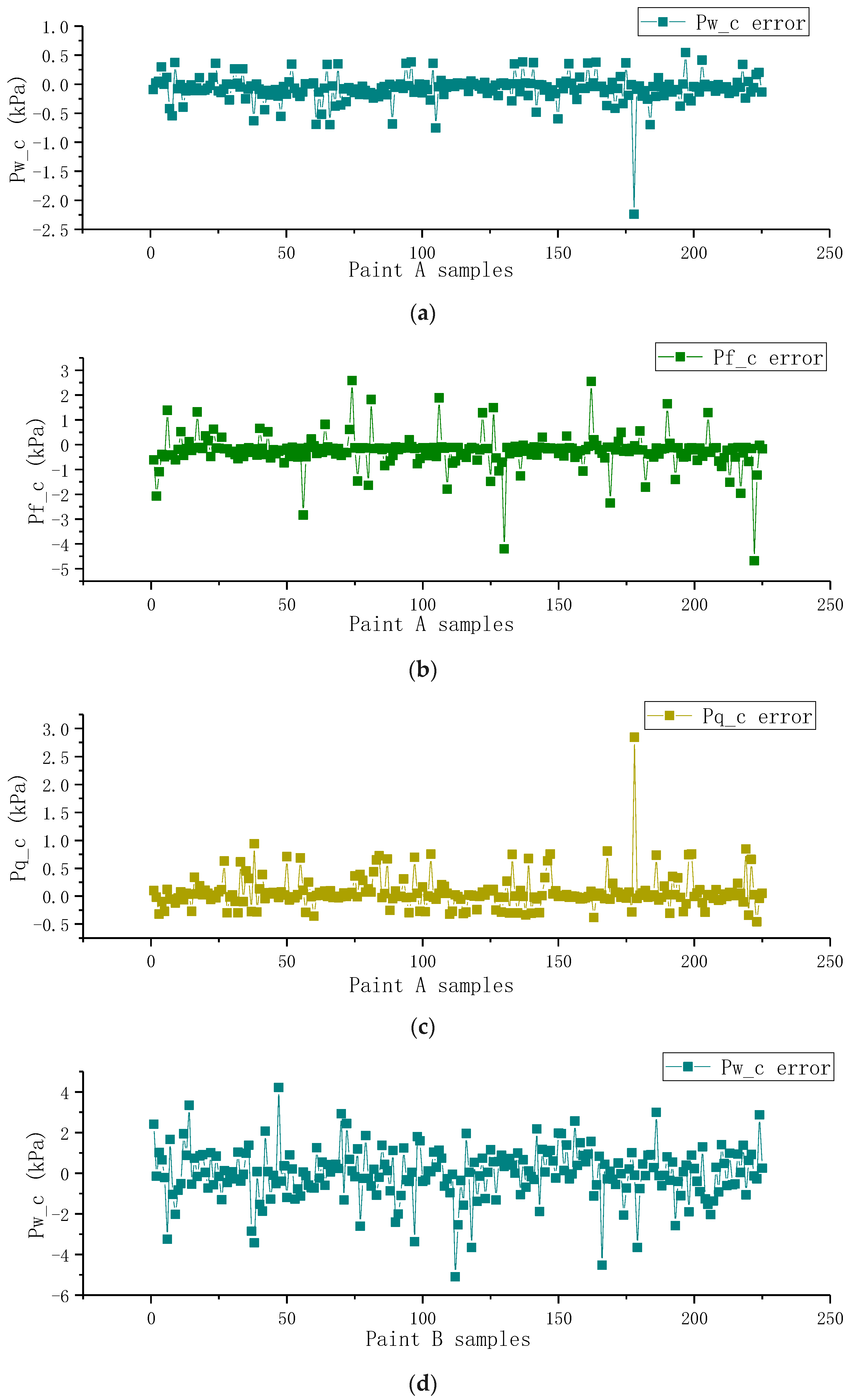
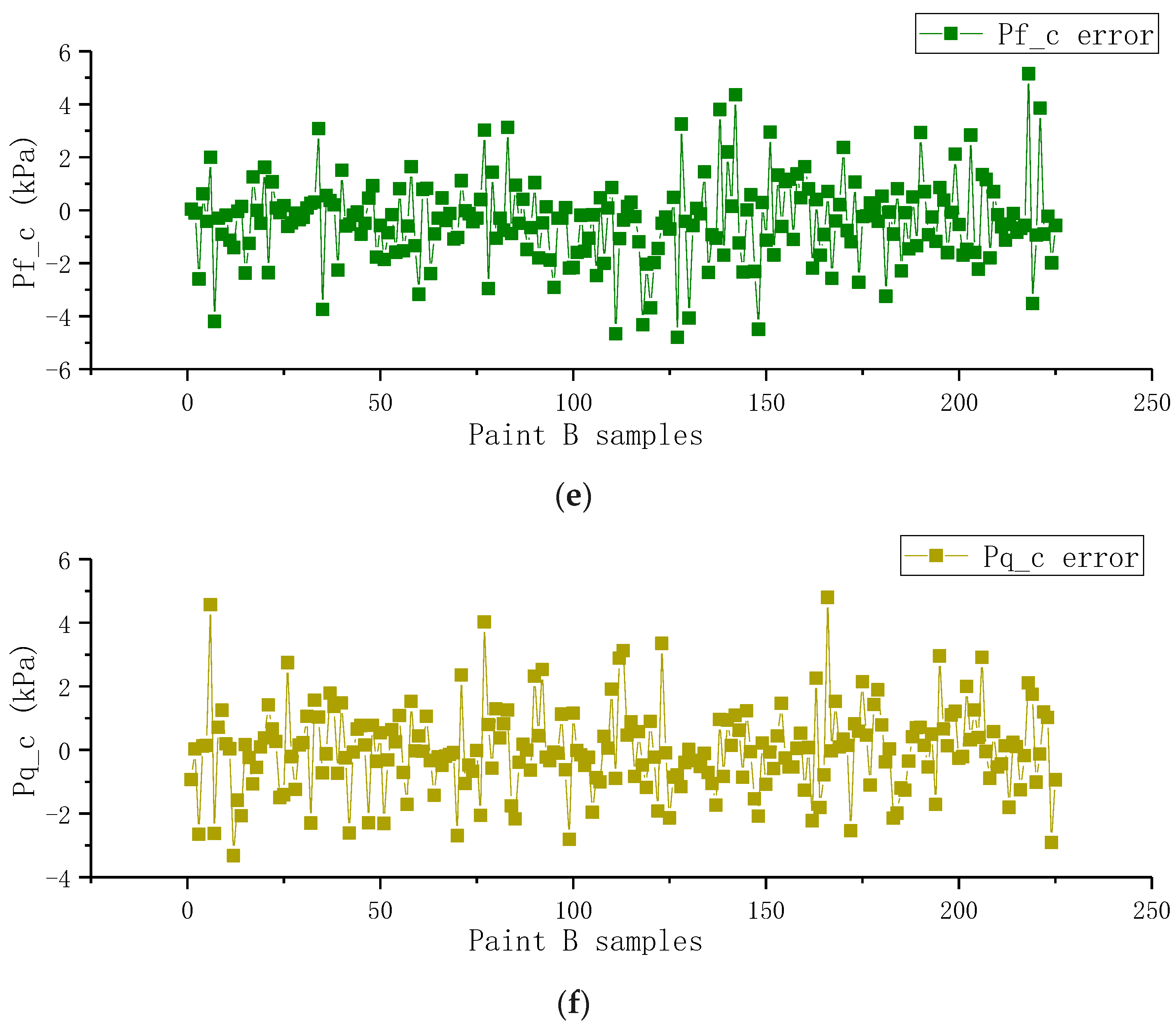
4.2. Image Difference Model Verification Results
5. Conclusions
- (1)
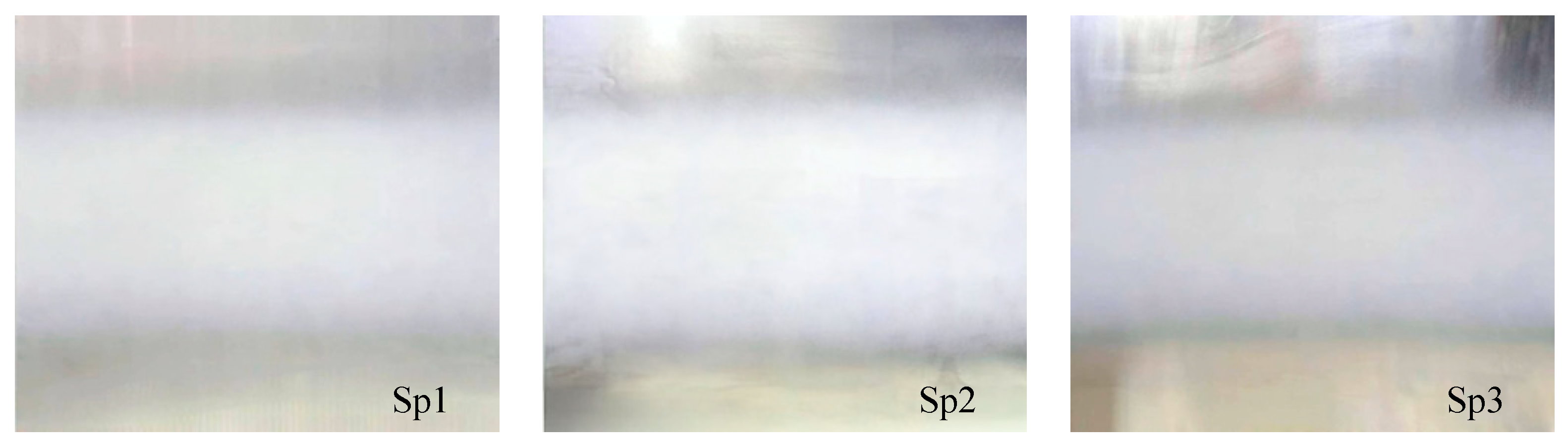
- Using the Arrhenius equation and the Hagen–Poiseuille equation, it was demonstrated that the datasets for pressure regulation and temperature variation are equivalent in terms of the conditions under which they were established. Experimental results indicate that, under conditions where temperature increase (18 °C vs. 24.1 °C) leads to reduced paint viscosity, optimizing spray pressure parameters (, , ) can effectively compensate for the effects of temperature changes, ensuring that the coating thickness distribution (Sp3) remains consistent with the low-temperature baseline (Sp1). This finding indicates that dynamic adjustment of pressure parameters can serve as a compensation mechanism for temperature fluctuations, thereby maintaining the stability of the spraying process without relying on strict temperature control. This method significantly reduces the high cost and complexity of environmental temperature control, while minimizing data collection biases caused by temperature fluctuations, providing a theoretical basis and feasible solution for optimizing industrial spraying processes.
- (2)
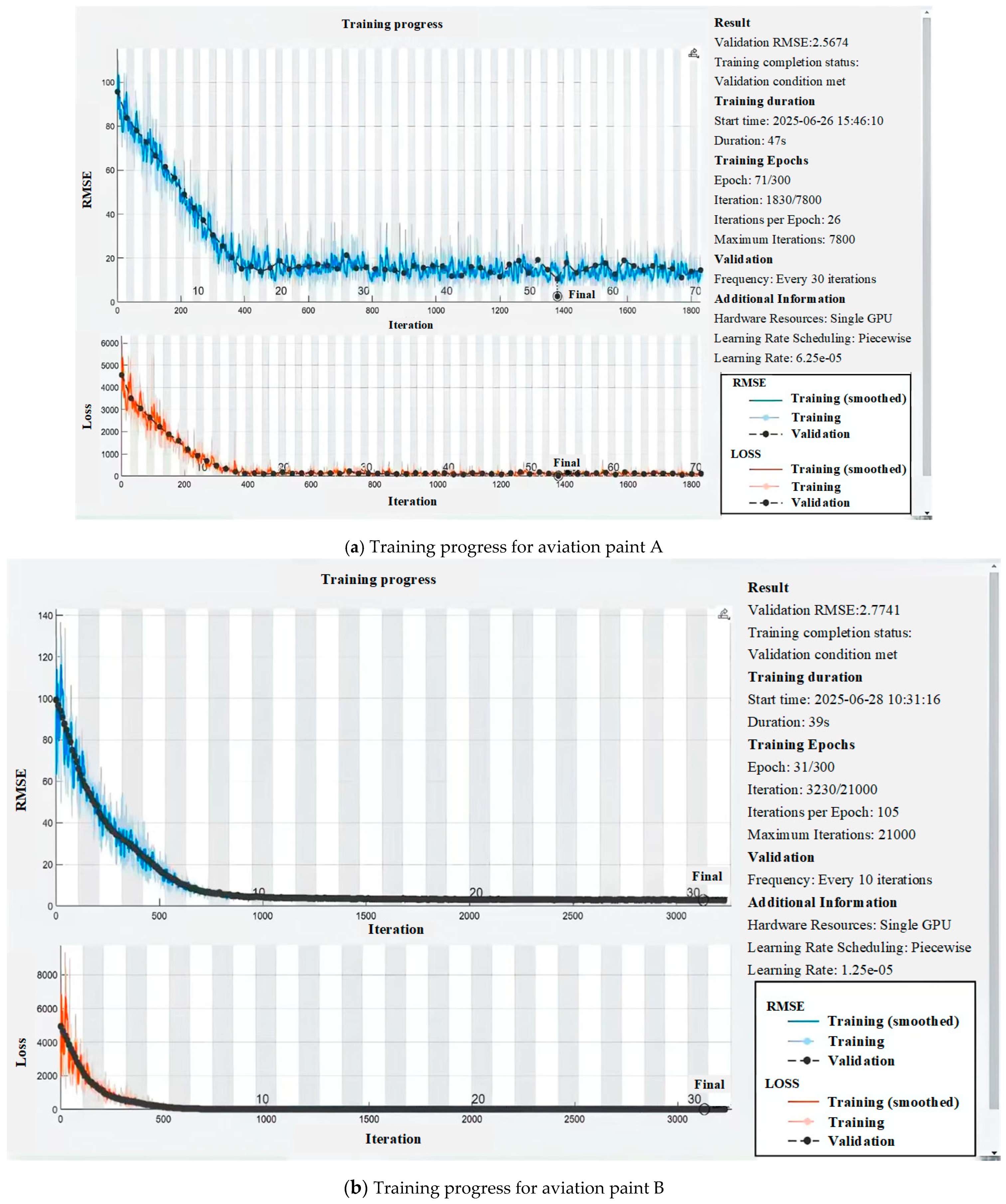
- This study employs online image data modeling coupled with real-time feedback to achieve modeling completion within 4 min (Table 9) while maintaining exceptional prediction accuracy ( > 0.999, Table 8), enabling real-time stabilization of the coating accumulation model in non-stationary environments.
- (3)
- The model adopts a dual-branch CNN + MLP architecture, which enhances features through image difference technology to predict pressure correction values. Optimization strategies (such as dynamic learning rate, dropout, and L2 regularization) further improve model performance. Two typical types of aviation paint materials were adopted in the experiment: high-viscosity polyurethane enamel (A, viscosity 22 s) and epoxy polyamide primer (B, viscosity 18 s). The results showed that the model achieved an R2 > 0.999 RMSE < 0.79 kPa, and σe < 0.74 kPa on the test set for aviation paint A, and an R2 > 0.997 RMSE < 0.67 kPa, and σe < 0.66 kPa on the test set for aviation paint B. Under the tested conditions, the dual-branch CNN + MLP model demonstrated superior performance and high accuracy in parameter prediction for both paint types through image differentiation and optimization strategies. This verifies its ability to achieve good dynamic adjustment performance for paints with different rheological properties in non-stable environments. However, verification is needed in a broader space.
Author Contributions
Funding
Institutional Review Board Statement
Informed Consent Statement
Data Availability Statement
Conflicts of Interest
Appendix A

| Sample | Sp1/μm | Sp2/μm | Sp3/μm |
|---|---|---|---|
| 1 | 1.8 | 4.1 | 2.6 |
| 2 | 2.1 | 4.9 | 2.4 |
| 3 | 2.4 | 3.5 | 2.3 |
| 4 | 2.9 | 4.7 | 4.3 |
| 5 | 4.8 | 5.8 | 5.1 |
| 6 | 5.1 | 6.7 | 6.1 |
| 7 | 6.5 | 9.7 | 7.3 |
| 8 | 7.4 | 11.6 | 9.2 |
| 9 | 8.2 | 13.8 | 11.9 |
| 10 | 11.4 | 15.4 | 13.5 |
| 11 | 13.4 | 15.9 | 14.6 |
| 12 | 15.4 | 17.2 | 15.7 |
| 13 | 17.9 | 19.1 | 16.1 |
| 14 | 17.6 | 20.2 | 18.3 |
| 15 | 19.5 | 21.6 | 18.9 |
| 16 | 19.2 | 21.5 | 18.5 |
| 17 | 18.5 | 20.9 | 18.0 |
| 18 | 17.5 | 19.8 | 16.8 |
| 19 | 16.2 | 18.2 | 16.5 |
| 20 | 13.8 | 16.5 | 14.4 |
| 21 | 13.9 | 16.5 | 13.8 |
| 22 | 10.9 | 13.6 | 12.5 |
| 23 | 9.2 | 12.0 | 10.8 |
| 24 | 6.2 | 10.7 | 9.6 |
| 25 | 7.1 | 8.9 | 6.9 |
| 26 | 5.0 | 7.3 | 6.7 |
| 27 | 3.5 | 6.9 | 6.5 |
| 28 | 3.2 | 5.4 | 4.6 |
| 29 | 2.5 | 4.0 | 4.0 |
| 30 | 2.0 | 3.4 | 4.2 |
References
- Paturi, U.M.R.; Cheruku, S.; Geereddy, S.R. Process modeling and parameter optimization of surface coatings using artificial neural networks (ANNs): State-of-the-art review. Mater. Today Proc. 2021, 38, 2764–2774. [Google Scholar] [CrossRef]
- Yu, D.; Su, C.; Wang, E.; Bao, H.; Qu, F. Method of 3D Coating Accumulation Modeling Based on Inclined Spraying. Sensors 2024, 24, 1212. [Google Scholar] [CrossRef] [PubMed]
- Sarikaya, O. Effect of the substrate temperature on properties of plasma sprayed Al2O3 coatings. Mater. Des. 2005, 26, 53–57. [Google Scholar] [CrossRef]
- Li, W.; Xue, N.; Shao, L.; Wu, Y.; Qiu, T.; Zhu, L. Effects of spraying parameters and heat treatment temperature on microstructure and properties of single-pass and single-layer cold-sprayed Cu coatings on Al alloy substrate. Surf. Coat. Technol. 2024, 490, 131184. [Google Scholar] [CrossRef]
- Ndiithi, N.J.; Min, K.; Mbugua, G.B.V.J.J.H.S. Optimizing Parameters of Arc-Sprayed Fe-Based Coatings Using the Response Surface Methodology. J. Therm. Spray Technol. 2023, 32, 2202–2220. [Google Scholar] [CrossRef]
- Paturi, U.M.R.; Reddy, N.S.; Cheruku, S.; Narala, S.K.R.; Cho, K.K.; Reddy, M.M. Estimation of coating thickness in electrostatic spray deposition by machine learning and response surface methodology. Surf. Coat. Technol. 2021, 422, 127559. [Google Scholar] [CrossRef]
- Shi, T.; Xu, J.; Cui, J.; Tao, L.; Xu, W.; Wang, Z.; Ji, J. Variable Velocity Coating Thickness Distribution Model for Super-Large Planar Robot Spraying. Coatings 2023, 13, 1434. [Google Scholar] [CrossRef]
- Nieto Bastida, S.; Lin, C.-Y. Autonomous trajectory planning for spray painting on complex surfaces based on a point cloud model. Sensors 2023, 23, 9634. [Google Scholar] [CrossRef] [PubMed]
- Liu, M.; Wu, H.; Yu, Z.; Liao, H.; Deng, S. Description and prediction of multi-layer profile in cold spray using artificial neural networks. J. Therm. Spray Technol. 2021, 30, 1453–1463. [Google Scholar] [CrossRef]
- Gui, L.; Wang, B.; Cai, R.; Yu, Z.; Liu, M.; Zhu, Q.; Xie, Y.; Liu, S.; Killinger, A. Prediction of in-flight particle properties and mechanical performances of HVOF-sprayed NiCr–Cr3C2 coatings based on a hierarchical neural network. Materials 2023, 16, 6279. [Google Scholar] [CrossRef] [PubMed]
- Bobzin, K.; Heinemann, H.; Dokhanchi, S.R. Development of an Expert System for Prediction of Deposition Efficiency in Plasma Spraying. J. Therm. Spray Technol. 2023, 32, 643–656. [Google Scholar] [CrossRef]
- Liu, M.; Yu, Z.; Wu, H.; Liao, H.; Zhu, Q.; Deng, S. Implementation of artificial neural networks for forecasting the HVOF spray process and HVOF sprayed coatings. J. Therm. Spray Technol. 2021, 30, 1329–1343. [Google Scholar] [CrossRef]
- Suryawanshi, S.; Bhosale, D.G.; Vasudev, H.; Prabhu, T.R. Back propagation model for prediction of deposition parameters in plasma sprayed WC-based coatings. Int. J. Interact. Des. Manuf. 2025, 19, 1837–1848. [Google Scholar] [CrossRef]
- Gerner, D.; Azarmi, F.; Mcdonnell, M.; Okeke, U. Application of Machine Learning for Optimization of HVOF Process Parameters. J. Therm. Spray Technol. 2024, 33, 504–514. [Google Scholar] [CrossRef]
- Ye, D.; Xu, Z.; Pan, J.; Yin, C.; Hu, D.; Wu, Y.; Li, R.; Li, Z. Prediction and analysis of the grit blasting process on the corrosion resistance of thermal spray coatings using a hybrid artificial neural network. Coatings 2021, 11, 1274. [Google Scholar] [CrossRef]
- Han, B.-Y.; Xu, W.-W.; Zhou, K.-B.; Zhang, H.-Y.; Lei, W.-N.; Cong, M.-Q.; Du, W.; Chu, J.-J.; Zhu, S. Performance analysis of plasma spray Ni60CuMo coatings on a ZL109 via a back propagation neural network model. Surf. Coat. Technol. 2022, 433, 128121. [Google Scholar] [CrossRef]
- Ling, L.; Zhang, X.; Hu, X.; Fu, Y.; Yang, D.; Liang, E.; Chen, Y. Research on spraying quality prediction algorithm for automated robot spraying based on KHPO-ELM neural network. Machines 2024, 12, 100. [Google Scholar] [CrossRef]
- Ye, W.; Wang, W.; Su, Y.; Qi, W.; Feng, L.; Xie, L. Prediction of HVAF thermal spraying parameters and coating properties based on improved WOA-ANN method. Microelectron. J. 2024, 39, 109265. [Google Scholar] [CrossRef]
- Zhu, H.; Li, D.; Yang, M.; Ye, D. Prediction of Microstructure and Mechanical Properties of Atmospheric Plasma-Sprayed 8YSZ Thermal Barrier Coatings Using Hybrid Machine Learning Approaches. Coatings 2023, 13, 15. [Google Scholar] [CrossRef]
- Deng, Z.; Chen, T.; Wang, H.; Li, S.; Liu, D. Process Parameter Optimization When Preparing Ti(C, N) Ceramic Coatings Using Laser Cladding Based on a Neural Network and Quantum-Behaved Particle Swarm Optimization Algorithm. Appl. Sci. 2020, 10, 6331. [Google Scholar] [CrossRef]
- Mahendru, P.; Tembely, M.; Dolatabadi, A. Artificial intelligence models for analyzing thermally sprayed functional coatings. J. Therm. Spray Technol. 2023, 32, 388–400. [Google Scholar] [CrossRef]
- Ye, D.; Wang, W.; Xu, Z.; Yin, C.; Zhou, H.; Li, Y. Prediction of thermal barrier coatings microstructural features based on support vector machine optimized by cuckoo search algorithm. Coatings 2020, 10, 704. [Google Scholar] [CrossRef]
- Chu, Y.-M.; Jakeer, S.; Reddy, S.; Rupa, M.L.; Trabelsi, Y.; Khan, M.I.; Hejazi, H.A.; Makhdoum, B.M.; Eldin, S.M. Double diffusion effect on the bio-convective magnetized flow of tangent hyperbolic liquid by a stretched nano-material with Arrhenius Catalysts. Case Stud. Therm. Eng. 2023, 44, 102838. [Google Scholar] [CrossRef]
- Wang, Y.; Xie, C. Uniform structural stability of Hagen–Poiseuille flows in a pipe. Commun. Math. Phys. 2022, 393, 1347–1410. [Google Scholar] [CrossRef]
- Kaur, R.; Karmakar, G.; Xia, F.; Imran, M. Deep learning: Survey of environmental and camera impacts on internet of things images. Artif. Intell. Rev. 2023, 56, 9605–9638. [Google Scholar] [CrossRef] [PubMed]
- van Bommel, W. Light Distribution; Springer: Berlin/Heidelberg, Germany, 2023; pp. 1048–1050. [Google Scholar]
- Przybył, K.; Koszela, K. Applications MLP and other methods in artificial intelligence of fruit and vegetable in convective and spray drying. Appl. Sci. 2023, 13, 2965. [Google Scholar] [CrossRef]
- Dominguez-Caballero, J.; Ayvar-Soberanis, S.; Curtis, D. Intelligent real-time tool life prediction for a digital twin framework. J. Intell. Manuf. 2025, 36, 1–21. [Google Scholar] [CrossRef]
- Liu, M.; Yu, Z.; Zhang, Y.; Wu, H.; Liao, H.; Deng, S. Prediction and analysis of high velocity oxy fuel (HVOF) sprayed coating using artificial neural network. Surf. Coat. Technol. 2019, 378, 124988. [Google Scholar] [CrossRef]


| ρ | Adjustment Items | Adjust Direction | Theoretical Basis |
|---|---|---|---|
| Decrease | Pw | Decrease | Low viscosity → High fluidity → Pressure must be reduced to balance flow |
| Pf | Decrease | Increased volume → Increased paint mist cone angle → Pressure must be reduced | |
| Pq | Increases | Compensate for atomization effects and avoid oversized spray particles. | |
| Increases | Same as above | Reverse adjustment | Maintain symmetry with the above logic. |
| Group | T/°C | ρ/s | Sp | Pw/kPa | Pf/kPa | Pq/kPa | Other Relevant Parameters |
|---|---|---|---|---|---|---|---|
| 1 | 18.5 | 22.16 | Sp1 | 180 | 120 | 150 | Same |
| Sp2 | 180 | 120 | 150 | ||||
| 2 | 24.1 | 17.62 | Sp3 | 200 | 110 | 100 |
| Model | Resolution | Frame Rate (fps) | Shutter Type | Volume (mm3) | Min Exposure (us) | Key Defect |
|---|---|---|---|---|---|---|
| MER2-301-125U3M-L | 2048 × 1536 | 125 | Global | 29 × 29 × 29 | 1 | |
| Basler ace2 2440 | 2448 × 2048 | 75 | Global | 32 × 32 × 42 | 1 | Insufficient frame rate, unable to meet the dynamic capture requirements of paint mist monitoring |
| Haikang MV-CE200 | 2048 × 1536 | 150 | Global | 29 × 29 × 42 | 2 | Rolling shutter causes exposure gaps, affecting image quality. |
| FLIR BFS-U3-16S2M | 1440 × 1080 | 164 | Global | 26 × 26 × 30 | 2 | Insufficient resolution, unable to meet the requirements for accurately distinguishing paint mist particles. |
| Performance | Paint A | Paint B |
|---|---|---|
| Viscosity (25 °C, s) | 22 ± 1.5 | 18 ± 1 |
| Solid content (%) | 65 ± 2 | 55 ± 3 |
| Applicable temperature (°C) | 15–30 | 18–30 |
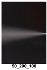
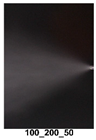
| Image_1 | Image_2 | /kPa | /kPa | /kPa |
|---|---|---|---|---|
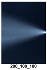 |  | 100 | 0 | 0 |
 | 50 | 0 | 0 | |
 | 0 | 0 | 50 | |
 | 0 | 0 | −150 | |
 | 0 | −50 | 0 |
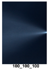
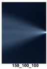
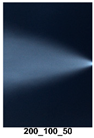
| Image_1 | Image_2 | /kPa | /kPa | /kPa |
|---|---|---|---|---|
 |  | 150 | −100 | 0 |
 | 100 | −100 | 50 | |
 | 100 | −100 | 0 | |
 | −50 | 0 | 0 | |
 | −50 | −100 | 0 |
| Parameters | Aviation Paint A | Aviation Paint B | ||||
|---|---|---|---|---|---|---|
| R2 | 0.99995 | 0.9998 | 0.9999 | 0.9989 | 0.9994 | 0.9966 |
| RMSE | 0.23980 | 0.86101 | 0.24336 | 0.6687 | 0.7536 | 0.6226 |
| σe | 0.22315 | 0.8563 | 0.23264 | 0.66788 | 0.7479 | 0.52176 |
| Parameters | Aviation Paint A | Aviation Paint B | ||||
|---|---|---|---|---|---|---|
| R2 | 0.99996 | 0.99984 | 0.99992 | 0.9988 | 0.9993 | 0.9979 |
| RMSE | 0.26677 | 0.79033 | 0.32678 | 0.6542 | 0.6696 | 0.6125 |
| σe | 0.2545 | 0.74442 | 0.31895 | 0.6513 | 0.6361 | 0.6123 |
| Steps | Time Consumption/min |
|---|---|
| Image Acquisition | 1.5 |
| Image capture and labelling | 1.4 |
| Image Difference Model Training | 1 |
| Model Testing | 0.005 |
| Totals | 3.905 |
Disclaimer/Publisher’s Note: The statements, opinions and data contained in all publications are solely those of the individual author(s) and contributor(s) and not of MDPI and/or the editor(s). MDPI and/or the editor(s) disclaim responsibility for any injury to people or property resulting from any ideas, methods, instructions or products referred to in the content. |
© 2025 by the authors. Licensee MDPI, Basel, Switzerland. This article is an open access article distributed under the terms and conditions of the Creative Commons Attribution (CC BY) license (https://creativecommons.org/licenses/by/4.0/).
Share and Cite
Su, C.; Yu, D.; Song, W.; Tian, H.; Bao, H.; Wang, E.; Li, M. Dynamic Control of Coating Accumulation Model in Non-Stationary Environment Based on Visual Differential Feedback. Coatings 2025, 15, 852. https://doi.org/10.3390/coatings15070852
Su C, Yu D, Song W, Tian H, Bao H, Wang E, Li M. Dynamic Control of Coating Accumulation Model in Non-Stationary Environment Based on Visual Differential Feedback. Coatings. 2025; 15(7):852. https://doi.org/10.3390/coatings15070852
Chicago/Turabian StyleSu, Chengzhi, Danyang Yu, Wenyu Song, Huilin Tian, Haifeng Bao, Enguo Wang, and Mingzhen Li. 2025. "Dynamic Control of Coating Accumulation Model in Non-Stationary Environment Based on Visual Differential Feedback" Coatings 15, no. 7: 852. https://doi.org/10.3390/coatings15070852
APA StyleSu, C., Yu, D., Song, W., Tian, H., Bao, H., Wang, E., & Li, M. (2025). Dynamic Control of Coating Accumulation Model in Non-Stationary Environment Based on Visual Differential Feedback. Coatings, 15(7), 852. https://doi.org/10.3390/coatings15070852