Abstract
In the structural integrity assessment of pipelines with multiple defects, conventional methods such as the DNV and MTI approaches demonstrate notable predictive biases. Specifically, the burst capacity estimated by the MTI model frequently exceeds experimental test values, whereas DNV calculations tend to be overly conservative, possibly resulting in unnecessary maintenance expenses. To address these challenges, this study employs nonlinear finite element analysis to reassess the failure pressure of pipelines with multiple corrosion defects. Initially, the interaction limit spacing between adjacent corrosion defects is computed to determine their potential for interaction. For adjacent corrosion defects exhibiting interaction, a merging limit criterion is introduced to evaluate their feasibility for merging. For those adjacent defects that satisfy the merging limit criterion, the DNV method is employed to merge them, followed by recalculating the failure pressure using the relevant formula. Finally, this study proposes a novel approach for assessing the failure pressure of pipelines with multiple corrosion defects. Through comparative analysis and validation, the proposed evaluation method exhibits enhanced accuracy in predicting the failure pressure of pipelines with multiple corrosion defects. The findings of this study provide a more precise methodology for assessing the residual strength of pipelines affected by multiple corrosion defects.
1. Introduction
Oil and gas pipelines provide substantial advantages in terms of low transportation costs, convenience, and efficiency, establishing them as a crucial component in the development of oil and gas fields [1,2]. However, with prolonged operation, the occurrence of corrosion damage becomes inevitable, leading to localized stress concentration as a result of wall thinning [3,4,5]. Consequently, conducting quantitative analyses and calculations to precisely evaluate the failure pressure of corroded pipelines is of critical importance. These assessments offer a theoretical basis for determining the continued operational feasibility of pipelines in service, while simultaneously reducing the risk of leakage incidents caused by corrosion [6].
In practical engineering applications, pipeline corrosion defects are predominantly multi-corrosion defects with complex geometries [7]. In cases involving multiple corrosion defects, there may exist interactions between any two groups of corrosion defects, which can further decrease the failure pressure of pipelines with corrosive flaws [8]. The study on the correlation among neighboring corrosion defects usually proposes interaction rules [9]. In the 1990s, Kiefner first proposed the concept of interactions and proposed three permutations of interactions [10,11]. DNV provides a set of interaction criteria based on experimental tests and finite element simulations, taking into account that the interaction is primarily influenced by pipe diameter and wall thickness. In the longitudinal direction, the interaction rule is Sc = 2(Dt)0.5; in the circumferential direction, the interaction rule is Sc = π(Dt)0.5 [12,13]. According to the interaction rules proposed by O’Grady II, the longitudinal limit spacing is 25.4 mm, and the circumferential limit spacing is six times the wall thickness [14,15,16]. The different interaction rules of various codes will affect the calculation result of failure pressure.
The DNV method refers to the approach outlined in the recommended practice DNV-RP-F101 “Corroded Pipelines,” published by the Norwegian Classification Society (DNV) [12]. DNV-RP-F101 provides comprehensive guidelines for evaluating individual defects, interacting defect groups (including defect projection, interaction assessment, and merging criteria), as well as complex-shaped defects. Its computational characteristics are typically conservative, meaning that the calculated failure pressure value is usually lower than or equal to the actual pipeline failure pressure, thereby ensuring an adequate safety margin for engineering applications [17,18]. The MTI method was developed by Benjamin and Cunha [19,20]. The MTI method is also an empirical formula based on the statistical analysis of a large number of pipelines blasting test data. Compared with the DNV method, the MTI method tends to yield results that are often closer to or slightly higher than the actual blasting test values when calculating the failure pressure of pipelines with corrosion defects, particularly for complex or interacting defect groups. This indicates that its level of conservatism is relatively low [21,22,23,24]. Additionally, this method provides criteria for assessing defect interactions and merging.
This study systematically reviews the failure assessment criteria proposed by DNV and MTI for multi-corrosion defects and critically examines the limitations of these two methods in evaluating the failure pressure of pipeline multi-corrosion defects. In view of the limitations of the original method, this study utilizes nonlinear finite element simulation to investigate the interaction criteria between short and long corrosion defects, thereby determining whether interactions exist among corrosion defects. For corrosion-defected pipelines exhibiting interaction, the merging limit criteria for short and long corrosion defects are individually evaluated to ascertain their suitability for merging. Consequently, a novel method for calculating the failure pressure of pipelines with multiple corrosion defects is proposed. This approach is subsequently compared with the DNV and MTI methods to verify its accuracy. A distinguishing feature of this method is that it redefines the interaction limit spacing coefficient, specifically the axial and circumferential interaction limit spacing for adjacent short and long corrosion defects, by integrating the interaction criteria from DNV and MTI and employing the finite element analysis approach. Furthermore, it investigates the deviation coefficient before and after the merger, which corresponds to the corrosion defect merging spacing. Based on these findings, a practicable failure pressure evaluation method grounded in a secondary assessment criterion is established.
2. Discussion of DNV Method and MTI Method
2.1. The Summary of DNV Method and MTI Method
The primary methods for calculating the failure pressure of pipelines with multiple corrosion defects are the DNV and MTI approaches. Both evaluation methods adopt the following steps to estimate the burst strength of pipelines with multiple defect occurrences [12,19]:
Step 1: Multiple corrosion defects are grouped because there is no interaction between defects in two adjoining groups;
Step 2: All corrosion defects are projected in both the axial and circumferential directions. If the projections of these defects overlap, the defects are treated as multiple single corrosion defects with varying depths;
Step 3: Count the interaction rules of adjoining defects. When the adjacent defects do not influence each other, the formula of failure pressure, which is used for a pipeline with a solitary corrosion flaw, calculates the failure pressure of multiple corroded defect Pipelines. When the adjacent defects exhibit mutual influence, corrosion defects are combined, and Table 1 shows the procedure for DNV and MTI to calculate the combined effective length, width, and depth.

Table 1.
Effective spacing of DNV and MTI.
The combined defect nm is defined by a single defect n to a single defect m, where n = 1 … N and m = n … N; i is Isolated defect number in a colony of N interacting defects; si is Longitudinal spacing between adjacent defects forming part of a colony of interacting defects (mm); Group is the defect group; k is a specific defect group; SL is the axial spacing of two defects, and SC is the circumferential spacing of two defects. For the DNV method, the effective length is defined as the combined length of the corresponding corrosion defect and the intervening non-corroded segment. The adequate depth is determined by employing the effective area method. For the MTI method, the effective size corresponds to the effective length in the DNV method, whereas the effective width includes the total width of multiple defects as well as the width of the non-corroded region between these defects. The adequate depth for this method is calculated using the effective volume approach.
Based on the defect’s effective length, depth, and width, the failure pressure evaluation formula for a single defect is applied to determine the failure pressure for each case, as shown in the formula.
2.2. Comparison of DNV Method and MTI Method
By comparing the failure pressure obtained from the tests with the pressure calculated according to the standard, this study evaluates the limitations of the DNV and MTI methods. Chouchaoui et al. from the University of Waterloo in Canada conducted burst tests on pipelines with multiple corrosion defects [25,26]. This research selected a representative set of burst tests. Benjamin et al. performed a series of thirty burst tests, from which seven representative test sets were chosen [19,27]. The failure pressure under various circumstances is shown in Table 2.
Table 2.
Failure pressure of eight groups of samples.
The failure pressure calculated by DNV and MTI is compared with the failure pressure of the burst test, respectively, and the scatter diagram is drawn, as shown in Figure 1.
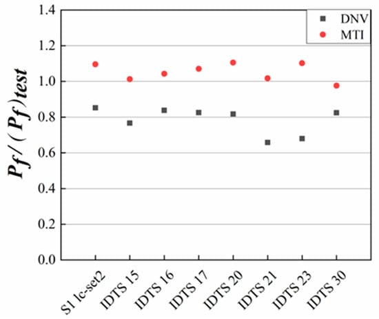
Figure 1.
The ratio of the standard predicted value to the burst test value.
Table 2 and Figure 1 demonstrate that the failure pressure calculated using the MTI method is generally higher than the burst test pressures, which may render the calculation results potentially unsafe. In contrast, the failure pressure estimated by the DNV method is consistently lower than the burst test pressures, indicating that the DNV predictions are conservative and thus safer. However, when multiple corrosion defects are cumulatively present in the circumferential direction over an extended period, as observed in samples IDTS 21 and IDTS 23, the DNV method becomes overly conservative. This may result in unnecessary inspections and potential resource wastage.
Under the premise of ensuring safety, this study employs the combination rules of the DNV method. To enhance the accuracy of failure pressure calculations, a novel approach for determining failure pressure based on the DNV combination method is proposed.
3. A New Method for Calculating Failure Pressure
3.1. Determination of Interaction Limit Spacing
The study of failure pressure typically involves determining the interaction limit spacing. To evaluate the interaction limit spacing, the interaction coefficient k is defined, which reflects the degree of interaction between two defects. The expression of the interaction coefficient k is as follows:
where and is the failure pressure of two adjoining corrosion defects with two spacing, and the unit is MPa; is the failure pressure after the combination of adjoining corrosion defects, and the unit is MPa.
3.1.1. Parameter Finite Element Analysis
- (1)
- Determination of failure criterion
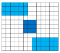
This article selects the nonlinear finite element analysis method. Firstly, the failure criterion is determined. Through many tests, Kirkwood et al. proved that the failure norm based on effective stress was highly accurate in predicting the failure pressure of pipelines with corrosion [28]. The expression of Von Mises’s effective stress was as follows [29]: For multi-corrosion defects with interaction, the multi-corrosion defect pipeline will fail when intact ligament CD reaches tensile strength and the remaining ligament AB does not reach tensile strength. For multi-corrosion defects without interaction, when the remaining ligament AB reaches the tensile strength, the multi-corrosion defect pipeline will fail [30], and the failure criterion of corrosion defect is shown in Figure 2.
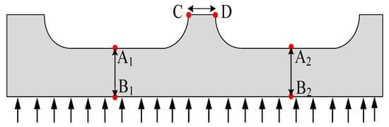
Figure 2.
Failure criterion diagram for corrosion defects.
- (2)
- Establishment of Geometric Model
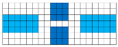
ABAQUS 6.14 software is capable of simulating the structural behavior of actual geometries of virtually any shape and accurately representing the mechanical properties of most common engineering materials. The pressure load is applied to the model, while the axial tension resulting from pipe end closure is imposed on the boundary surface nodes at the end. The end constraint is defined to permit movement exclusively along the X-axis. To mitigate the risk of stress concentration, all edges of the corrosion defects are processed using a chamfering technique. A radius equal to half of the defect depth is employed for the chamfering, as illustrated in Figure 3.
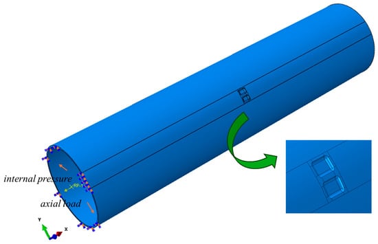
Figure 3.
Pipeline finite element model diagram.
- (3)
- Define material properties
The corrosion defect model of the oil and gas pipeline, initially constructed in SolidWorks 2020 software, is imported into Abaqus 6.14 finite element software. Following verification of the model’s accuracy, the material properties of the pipeline are assigned. The density is 7850 kg/m3, elastic modulus is 210 GPa, yield strength is 632 MPa, tensile strength is 698 MPa. In finite element analysis, selecting an appropriate constitutive model to construct the true stress–strain relationship of the material is essential. The Ramberg–Osgood constitutive model demonstrates superior performance in capturing the nonlinear behavior associated with corrosion interactions [31,32]. The expression of the stress–strain relationship is as follows:
where σR is the Ramberg–Osgood stress; n is the hardening coefficient of the material; E is the elastic modulus.
- (4)
- Mesh subdivision
The quality of the mesh significantly influences the accuracy of finite element simulation results. Grid independence verification is conducted to select an optimal grid configuration that ensures both simulation accuracy and computational efficiency. The method used is to model the blasting test of X80 pipeline with double corrosion defects (see Figure 4). Grid models with 3, 4, 5, and 6 layers through the wall thickness direction are, respectively, established. The total number of elements for each configuration is 10,867, 14,236, 17,786, and 21,336, as illustrated in Figure 5. Figure 6 shows the comparison of different mesh models. The first curve represents the variation of Mises stress at point O, the midpoint of the central axis AB on the residual ligament of the corrosion defect, under internal pressure; the second curve corresponds to the failure pressure. Figure 4 presents a comparison between the Mises stress distribution obtained from the finite element analysis and that observed in the actual pipeline at the moment of failure. It can be observed that the failure of the corroded pipeline occurs when the remaining wall thickness between the two corrosion defects reaches the material’s tensile strength.
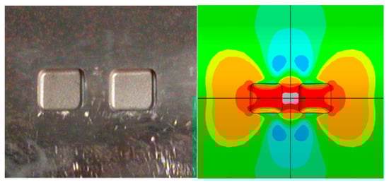
Figure 4.
Mises stress cloud diagram at failure time.
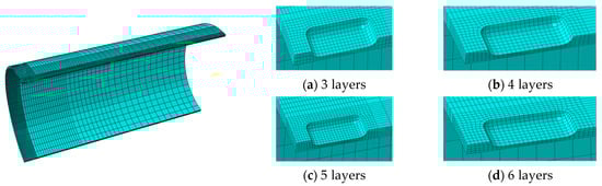
Figure 5.
Grid model.
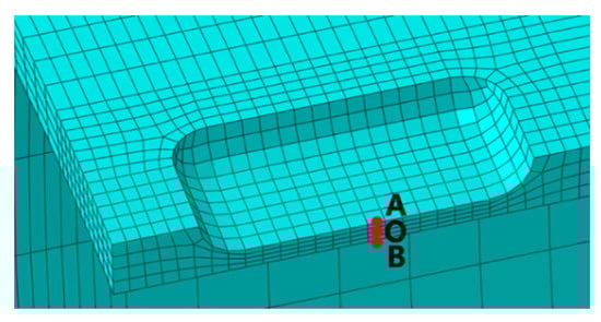
Figure 6.
Comparison content.
The extracted results are plotted as the Mises stress curve at point O with respect to internal pressure, as illustrated in Figure 7. It can be observed that as the internal pressure increases, the stress curves corresponding to the 3-layer, 4-layer, 5-layer, and 6-layer grid models essentially overlap, indicating that grids beyond three layers have negligible influence on the Mises stress distribution. The failure pressure determined using the Mises stress failure criterion is presented in Table 3. It can be observed that when the number of layers through the wall thickness direction reaches four, different mesh models fail at the same analysis step, resulting in a final converted failure pressure error of 4.18%. However, the error of the failure pressure calculated by the three-layer grid model increases to 5.17%. Combined with the British BS7910 failure standard [33], the four-layer grid is used.
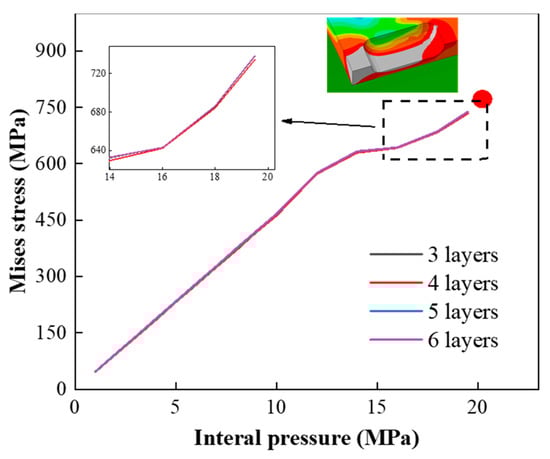
Figure 7.
The change of Mises stress with internal pressure at point O.
Table 3.
Comparison of results.
To make the research convenient, it is essential to carry on the dimensionless processing of the studied parameters. By summing up DNV-RP-F101 criteria [12] and ASME B31G criteria [34], the dimensionless expressions of corrosion depth are selected as , and the dimensionless expressions of corrosion length, corrosion width, longitudinal spacing, and circumferential spacing are, respectively, L/(Dt)0.5, w/(Dt)0.5, SL/(Dt)0.5 and SC/(Dt)0.5. Where D is the pipe diameter, the unit is mm; t is the pipe thickness, the unit is mm. At the same time, ASME B31G defines a short corrosion defect when the defect length is L < (20Dt)0.5. When the defect length is (20Dt)0.5 ≤ L ≤ (50Dt)0.5, it is a long corrosion defect.
The number of grid partitions should also be controlled in accordance with the balance between calculation accuracy and computational cost. In the grid division process, mesh refinement is applied near the corrosion defect area, while coarser meshing is utilized in regions farther from the corrosion defect area. Four layers of grid thickness are selected for the established corrosion-defect pipeline model based on a comparative analysis of results obtained from multiple grid divisions.
3.1.2. Interaction Limit Spacing in the Longitudinal Direction
The corrosion defects in the longitudinal direction are divided into two types: short longitudinal corrosion defects and long longitudinal corrosion defects. Figure 8 shows how the interaction coefficient varies with the longitudinal spacing of adjoining corrosion defects at different corrosion depths. As shown in the figure, the interaction coefficient decreases with the increase in longitudinal spacing, indicating that the interaction between adjacent defects becomes progressively weaker. Under the same corrosion depth, the rate of change of the interaction coefficient for short defects is greater than that for long corrosion defects, suggesting that the interaction between short defects is more sensitive to changes in size.
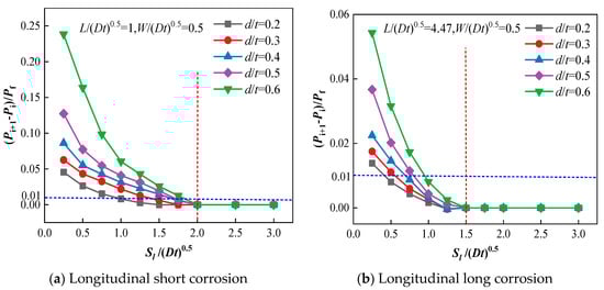
Figure 8.
Variation of interaction coefficient with longitudinal spacing.
For short defects, when the longitudinal spacing is Sl/(20Dt)0.5 = 0.25, the interaction coefficient increases with the growth of corrosion depth, indicating that the corrosion depth will promote the interaction at this time. However, when the longitudinal spacing increases, the rate of change of the interaction coefficient for corrosion defects at greater depths is more pronounced compared to those at shallower depths. This indicates that deeper defects are more likely to induce larger fluctuating stress changes, thereby rendering the corrosion defects more susceptible to failure. A similar conclusion can be drawn for long corrosion-defect pipelines.
According to experience, when k = 0.01, the corresponding spacing is the interaction limit spacing. When the gap between adjacent defects exceeds the interaction limit spacing, no interaction is observed between the adjacent corrosion defects. Otherwise, interaction is observed between these defects.
When the corrosion defect depth coefficient is 0.2, 0.3, 0.4, 0.5, and 0.6, the interaction limit spacing corresponding to adjoining short corrosion defects in the longitudinal direction is (Dt)0.5, 1.25(Dt)0.5, 1.5(Dt)0.5, 1.75(Dt)0.5, and 2(Dt)0.5, and the interaction limit spacing corresponding to adjoining long corrosion defects is 0.25(Dt)0.5, 0.5(Dt)0.5, 0.75(Dt)0.5, 0.75(Dt)0.5, and (Dt)0.5, as shown in Table 3. Therefore, the longitudinal limit spacing of interaction between adjoining short defects is 2(Dt)0.5, and the longitudinal limit spacing between adjoining long defects is 0.75(Dt)0.5, which is the criterion for judging whether there is interaction between adjoining defects in the longitudinal direction.
From Table 4, the interaction limit spacing for adjacent long corrosion defects is observed to decrease in comparison to that for adjacent short corrosion defects. This indicates that the degree of correlation among neighboring corrosion defects diminishes as the length of the corrosion defects increases.
Table 4.
Longitudinal interaction limit spacing.
3.1.3. Interaction Rules in the Circumferential Direction
Corrosion defects in the circumferential direction are classified into two categories: short circumferential corrosion defects and long circumferential corrosion defects. Figure 9 demonstrates the variation of the interaction coefficient with respect to the circumferential spacing between adjacent corrosion defects at various corrosion depths. As depicted in the figure, the interaction coefficient decreases as the circumferential spacing increases, suggesting that the interaction between adjacent corrosion defects diminishes.
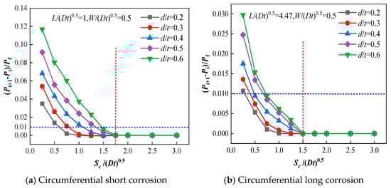
Figure 9.
The variation of interaction coefficient with circumferential spacing.
For short defects, when the circumferential spacing is Sc/(Dt)0.5 = 0.25, the interaction coefficient increases with the growth of corrosion depth, indicating that the corrosion depth will promote the interaction at this time. The same conclusion can be reached in the circumferential direction for long corroded defective pipes.
When the corrosion defect depth coefficients are 0.2, 0.3, 0.4, 0.5, and 0.6, respectively, the interaction limit spacing corresponding to adjoining short corrosion defects in the circumferential direction is 0.5(Dt)0.5, 0.75(Dt)0.5, (Dt)0.5, 1.25(Dt)0.5, and 1.5(Dt)0.5, and the interaction limit spacing corresponding to adjoining long corrosion defects is 0.25(Dt)0.5, 0.5(Dt)0.5, 0.5(Dt)0.5, 0.75(Dt)0.5, and 0.75(Dt)0.5, as shown in Table 5. Therefore, the circumferential limit spacing of interaction between adjoining short defects is 1.5(Dt)0.5, and the long defects is 0.75(Dt)0.5, which is the criterion for judging whether there is an interaction observed between adjacent defects in the circumferential direction. Together with the criterion in the longitudinal direction, this criterion serves as the primary criterion for failure pressure evaluation of pipelines with multiple defects.
Table 5.
Circumferential interaction limit spacing.
3.2. Determination of Combination Limit Spacing
In the case of interaction between adjacent defects, when the spacing between the defects is reduced to a certain threshold, the effect of the adjacent defects becomes similar to that of combined corrosion defects. The spacing at this point is defined as the combination limit spacing. This article defines the deviation coefficient E to assess the difference in failure pressure before the combination and after. The formula for E is as follows:
where is the failure pressure of the adjoining defects. is the failure pressure after the combination of the defects.
3.2.1. Combination Limit Spacing in the Longitudinal Direction
The combination limit spacing is investigated in two scenarios: short longitudinal corrosion defects and long longitudinal corrosion defects in the longitudinal direction. Figure 6 illustrates the variation of the failure pressure deviation coefficient E with respect to the longitudinal spacing of adjacent corrosion defects before and after combination at various corrosion depths. As shown in the figure, with the increase in longitudinal spacing, the failure pressure deviation before and after combination progressively increases, indicating that the combination becomes increasingly inappropriate.
For short defects, when the longitudinal spacing is SL/(Dt)0.5 < 0.4, the deeper the corrosion depth of adjoining defects is, the smaller the failure pressure deviation coefficient, indicating that adjoining corrosion defects are more suitable for combining. Long corrosion defects inspire the same conclusion.
According to experience, when E = 5%, the spacing is the combination limit spacing. When the spacing between adjoining defects is less than the combination limit spacing, there is complete interaction between adjoining defects. Otherwise, there is incomplete interaction.
According to Figure 10, when the depth coefficients of corrosion defects are 0.2, 0.3, 0.4, 0.5, and 0.6, respectively, the combination limit spacing corresponding to adjoining short corrosion defects in the longitudinal direction is (Dt)0.5, 0.75(Dt)0.5, 0.75(Dt)0.5, 0.5(Dt)0.5, and 0.5(Dt)0.5 respectively. The combination limit spacing corresponding to adjoining long corrosion defects in the longitudinal direction is 0.25(Dt)0.5. The data summary is shown in Table 6. Therefore, the longitudinal combination limit spacing of adjoining short corrosion defects is (Dt)0.5, and the longitudinal combination limit spacing of adjoining long defects is 0.25(Dt)0.5, which is the basis for judging whether adjoining corrosion defects are suitable for combining in the longitudinal direction.
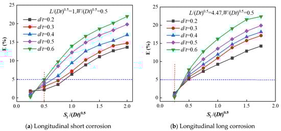
Figure 10.
Variation of E with longitudinal spacing.
Table 6.
Longitudinal combination limit spacing.
3.2.2. Combination Limit Spacing in the Circumferential Direction
The combination limit spacing is investigated in two scenarios: short longitudinal corrosion defects and long circumferential corrosion defects. Figure 11 illustrates the variation of the deviation coefficient before and after combination as a function of the circumferential spacing between adjacent corrosion defects at various corrosion depths. As shown in the figure, with the increase in circumferential spacing, the failure pressure deviation coefficient decreases both before and after the combination, suggesting that the combination becomes progressively less appropriate.
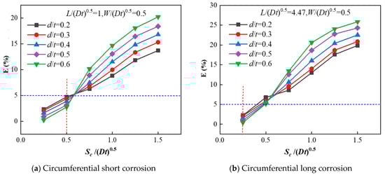
Figure 11.
Variation of E with circumferential spacing.
From Figure 11, when the depth coefficients of corrosion defects are 0.2, 0.3, 0.4, 0.5, and 0.6, respectively, the combination limit spacing corresponding to adjoining short defects in the circumferential direction is 0.5(Dt)0.5, and the combination limit spacing corresponding to adjoining long defects in the longitudinal direction is 0.25(Dt)0.5. The data is summarized in Table 7. This is the rule for determining whether the combination of adjacent defects in the circumferential direction is appropriate. Combined with the criterion in the longitudinal direction, it forms a secondary criterion for evaluating the failure pressure of pipelines with multiple corrosion defects.
Table 7.
Circumferential combination limit spacing.
3.3. Determination of Failure Pressure
Based on prior research, when calculating the failure pressure of multiple defects, adjacent defects are first projected and grouped according to specific criteria. These grouping criteria are derived from the secondary evaluation criteria: the primary level determines whether interaction exists between defects, while the secondary level assesses whether complete interaction occurs.
When the spacing between adjacent corrosion defects varies and simultaneously satisfies both the interaction limit spacing and the combination limit spacing, the failure pressure of each corrosion defect is calculated according to the method for a single corrosion defect.
When the spacing between adjacent defects satisfies both the interaction limit spacing and the combination limit spacing, it is determined that the adjacent corrosion defects can be combined. The combination criteria are implemented in accordance with DNV guidelines, and the failure pressure is calculated using the failure pressure formula specified in DNV.
As shown in the formula, the minimum failure pressure of all multi-corrosion defect combinations is taken as the failure pressure of the multiple defect pipeline.
4. Verification
For the eight groups of burst tests selected above, the failure pressure was calculated using the DNV method, the MTI method, and the approach proposed in this study, respectively. The calculation results are presented in Table 8. Additionally, error analysis was conducted on the eight groups of failure pressure data, and the corresponding results are summarized in Table 9.
Table 8.
Calculation results of failure pressure of multi-corrosion defects.
Table 9.
Error of calculation result of failure pressure for multi-corrosion defects.
To present the data more vividly, the tabulated data are visualized in a column chart, as illustrated in Figure 12 below. Both the figure and the table clearly demonstrate that, when calculating the failure pressure of corroded pipelines with defects, the results obtained using the method proposed in this study are consistently lower than those derived from burst tests, thereby aligning with safety standards. When there is complete interaction between adjacent corrosion defects, the failure pressure error calculated using this method is equivalent to that calculated using the DNV method. In cases of incomplete interaction between adjacent defects, the failure pressure error calculated using this method is smaller than that calculated using the DNV method, suggesting that this method can enhance the accuracy of failure pressure calculations for multi-corrosion defects to some extent.
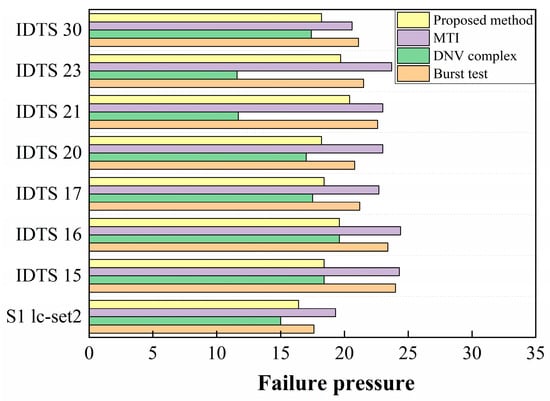
Figure 12.
Bar chart of test comparison.
5. Conclusions
1. This paper summarizes the methods for evaluating the failure pressure of multiple defects. Among these evaluation methods, the MTI method is considered unsafe due to its underestimation of effective depth. The DNV method employs a suitable combined effective spacing; however, its calculation results tend to be somewhat conservative.
2. The interaction limit spacing coefficient is defined to determine whether there is interaction between adjacent defects and serves as the primary criterion for assessing the maximum withstand pressure of pipelines with multiple flaws. The longitudinal interaction limit spacing of short corrosion defects is 2(Dt)0.5, and the circumferential interaction limit spacing is 1.5(Dt)0.5. The circumferential interaction limit spacing of long corrosion defects is (Dt)0.5, and the circumferential interaction limit spacing is 0.75(Dt)0.5.
3. The deviation coefficient before and after combination is defined to determine whether adjacent defects can be combined, serving as a secondary criterion for calculating the failure pressure of pipelines with multiple defects. The longitudinal combination limit spacing of short corrosion defects is (Dt)0.5, and the circumferential combined limit spacing is 0.5(Dt)0.5. The axial combined ultimate spacing of long corrosion defects is 0.25(Dt)0.5, and the circumferential combined ultimate spacing is 0.25(Dt)0.5.
4. By validating the burst test results, a failure pressure evaluation method based on secondary evaluation criteria is proposed. This method enhances the calculation accuracy of failure pressure through comparison with the burst test results.
Author Contributions
Conceptualization, J.C. and Y.Z.; methodology, J.C. and Y.C.; software, Y.Z. and Y.L.; validation, Y.Z. and Y.L.; formal analysis, Y.L.; investigation, D.Z.; resources, J.C., Y.Z. and Y.C.; data curation, D.Z.; writing—original draft preparation, D.Z. and Y.H.; writing—review and editing, Y.H.; visualization, Q.Z.; supervision, Q.Z.; project administration, Y.H.; funding acquisition, J.C. All authors have read and agreed to the published version of the manuscript.
Funding
This research was funded by the National Key R&D Program of China (Grant No. 2022YFC3070100), the Science and Technology Research Project of PipeChina (No. AQWH202301), the National Natural Science Foundation of China (12272412), the National Natural Science Foundation of China (12202502), the Shandong Provincial Natural Science Foundation, China (ZR2022QE039) and the Fundamental Research Funds for the Central Universities (23CX03002A, 24CX06008A).
Data Availability Statement
All data, models, and code generated or used during the study appear in the submitted article.
Conflicts of Interest
The all authors declare that the research was conducted in the absence of any commercial or financial relationships that could be construed as a potential conflict of interest.
References
- Sun, M.; Zhu, J.X.; Hao, S. Analyzing the Innovation Progress in Global Oil and Gas Pipeline Transportation. J. Pipeline Syst. Eng. Pract. 2025, 16, 04025007. [Google Scholar] [CrossRef]
- Chen, J.; Wu, X.; Jiang, Z.; Li, Q.; Zhang, L.; Chu, J.; Song, Y.; Yang, L. Application of machine learning to leakage detection of fluid pipelines in recent years: A review and prospect. Measurement 2025, 248, 116857. [Google Scholar] [CrossRef]
- Lu, H.; Iseley, T.; Behbahani, S.; Fu, L. Leakage detection techniques for oil and gas pipelines: State-of-the-art. Tunn. Undergr. Space Technol. 2020, 98, 103249. [Google Scholar] [CrossRef]
- Shao, X.; Cai, B.; Ahmed, S.; Zhou, X.; Hu, Z.; Sui, Z.; Liu, X. Towards proactive corrosion management: A predictive modeling approach in pipeline industrial applications. Process Saf. Environ. Prot. 2024, 190, 1471–1480. [Google Scholar] [CrossRef]
- Sun, M.; Li, X.; Liu, J. Determination of Folias factor for failure pressure of corroded pipeline. J. Press. Vessel Technol. 2020, 142, 031802. [Google Scholar] [CrossRef]
- Chen, Y.; Zhang, H.; Zhang, J.; Liu, X.; Li, X.; Zhou, J. Failure assessment of X80 pipeline with interacting corrosion defects. Eng. Fail. Anal. 2015, 47, 67–76. [Google Scholar] [CrossRef]
- Lu, H.; Peng, H.; Xu, Z.D.; Qin, G.; Azimi, M.; Matthews, J.C.; Cao, L. Theory and Machine Learning Modeling for Failure pressure Estimation of Pipeline with Multipoint Corrosion. J. Pipeline Syst. Eng. Pract. 2023, 14, 04023022. [Google Scholar] [CrossRef]
- Sun, M.; Fang, H.; Miao, Y.; Zhao, H.; Li, X. Experimental study on strain and failure location of interacting defects in pipeline. Eng. Fail. Anal. 2023, 148, 107119. [Google Scholar] [CrossRef]
- Zhang, Y.; Wang, W.; Shuai, J.; Shuai, Y.; Hua, L.; Lv, Z. A novel assessment method to identifying the interaction between adjoining corrosion defects and its effect on the burst capacity of pipelines. Ocean Eng. 2023, 281, 114842. [Google Scholar] [CrossRef]
- Kiefner, J.F.; Vieth, P.H. PC program speeds new criterion for evaluating corroded pipe. Oil Gas J. 1990, 90, 91–93. [Google Scholar]
- Kiefner, J.F.; Vieth, P.H. New method corrects criterion for evaluating corroded pipe. Oil Gas J. 1990, 88, 56–59. [Google Scholar]
- Det Norske Veritas. DNV-RP-F101 Corroded Pipelines. 2015. Available online: https://www.dnv.com/energy/standards-guidelines/dnv-rp-f101-corroded-pipelines/ (accessed on 25 June 2025).
- D’Aguiar, S.C.M.; de Siqueira Motta, R.; Afonso, S.M.B. An investigation on the collapse response of subsea pipelines with interacting corrosion defects. Eng. Struct. 2024, 321, 118911. [Google Scholar] [CrossRef]
- O’Grady, T.J.; Hisey, D.T.; Kiefner, J.F. A systematic method for the evaluation of corroded pipelines. Pipeline Eng. 1992, 46, 27–35. [Google Scholar]
- O’Grady, I.I.; Hisey, D.T.; Kiefner, J.F. Method for evaluating corroded pipe addresses variety of patterns. Oil Gas J. 1992, 90, 77–78, 80–82. [Google Scholar] [CrossRef]
- O’Grady, T.J.; Hisey, D.T.; Kiefner, J.F. Pressure calculation for corroded pipe developed. Oil Gas J. 1992, 90, 442. [Google Scholar]
- Choi, K.H.; Lee, C.S.; Ryu, D.M.; Koo, B.Y.; Kim, M.H.; Lee, J.M. Comparison of computational and analytical methods for evaluation of failure pressure of subsea pipelines containing internal and external corrosions. J. Mar. Sci. Technol. 2016, 21, 369–384. [Google Scholar] [CrossRef]
- Li, X.; Chen, G.; Liu, X.; Ji, J.; Han, L. Analysis and evaluation on residual strength of pipelines with internal corrosion defects in seasonal frozen soil region. Appl. Sci. 2021, 11, 12141. [Google Scholar] [CrossRef]
- Benjamin, A.C.; Freire, J.L.F.; Vieira, R.D. Part 6: Analysis of pipeline containing interacting corrosion defects. Exp. Tech. 2007, 31, 74–82. [Google Scholar] [CrossRef]
- Benjamin, A.C.; Freire, J.L.F.; Vieira, R.D.; Cunha, D.J. Interaction of corrosion defects in pipelines—Part 2: MTI JIP database of corroded pipe tests. Int. J. Press. Vessel. Pip. 2016, 145, 41–59. [Google Scholar] [CrossRef]
- Freire, J.L.; Vieira, R.D.; Fontes, P.M.; Benjamin, A.C.; Murillo C., L.S.; Miranda, A.C. The critical path method for assessment of pipelines with metal loss defects. In Proceedings of the International Pipeline Conference, Calgary, AB, Canada, 24–28 September 2012; American Society of Mechanical Engineers: New York, NY, USA, 2012; Volume 45134, pp. 661–671. [Google Scholar]
- Motta, R.D.S.; Afonso, S.M.; Willmersdorf, R.B.; Lyra, P.R.; de Andrade, E.Q. Automatic modeling and analysis of pipelines with colonies of corrosion defects. Mec. Comput. 2010, 29, 7871–7890. [Google Scholar]
- Benjamin, A.C.; Cunha, D.J. New method for the prediction of the collapse pressure of interacting corrosion defects. In Proceedings of the ISOPE International Ocean and Polar Engineering Conference, Lisbon, Portugal, 1–6 July 2007. ISOPE-I-07-171. [Google Scholar]
- Benjamin, A.C.; Freire, J.L.F.; Vieira, R.D.; Cunha, D.J. Interaction of corrosion defects in pipelines—Part 1: Fundamentals. Int. J. Press. Vessel. Pip. 2016, 144, 56–62. [Google Scholar] [CrossRef]
- Chouchaoui, B. Evaluating the Remaining Strength of Corroded Pipelines. Ph.D. Thesis, Department of Mechanical Engineering, University of Waterloo, Waterloo, ON, Canada, 1993; p. 3535. [Google Scholar]
- Chouchaoui, B.A.; Pick, R.J. A Three Level Assessment of the Residual Strength of Corroded Line Pipe; American Society of Mechanical Engineers: New York, NY, USA, 1994; No. CONF-940230. [Google Scholar]
- Benjamin, A.C.; Freire, J.L.F.; Vieira, R.D.; Diniz, J.L.; de Andrade, E.Q. Proceedings of the International Conference on Offshore Mechanics and Arctic Engineering, Halkidiki, Greece, 12–17 June 2005; American Society of Mechanical Engineers: New York, NY, USA; Volume 41979, pp. 403–417.
- Fu, B.; Kirkwood, M.G. Predicting Collapse Pressure of Internally Corroded Linepipe Using the Finite Element Method; American Society of Mechanical Engineers: New York, NY, USA, 1995; No. CONF-950695. [Google Scholar]
- Asgari, M.; Kouchakzadeh, M.A. An effective von Mises stress and corresponding effective plastic strain for elastic–plastic ordinary peridynamics. Meccanica 2019, 54, 1001–1014. [Google Scholar] [CrossRef]
- Al-Owaisi, S.S.; Becker, A.A.; Sun, W. Analysis of shape and location effects of closely spaced metal loss defects in pressurised pipes. Eng. Fail. Anal. 2016, 68, 172–186. [Google Scholar] [CrossRef]
- Benjamin, A.C.; de Andrade, E.Q.; Jacob, B.P.; Pereira, L.C.; Machado, P.R., Jr. Failure behavior of colonies of corrosion defects composed of symmetrically arranged defects. In Proceedings of the International Pipeline Conference 2006, Calgary, AB, Canada, 25–29 September 2006; Volume 42622, pp. 417–432. [Google Scholar]
- de Andrade, E.Q.; Benjamin, A.C.; Machado, P.R., Jr.; Pereira, L.C.; Jacob, B.P.; Carneiro, E.G.; Noronha, D.B., Jr. Finite element modeling of the failure behavior of pipelines containing interacting corrosion defects. In Proceedings of the International Conference on Offshore Mechanics and Arctic Engineering 2006, Hamburg, Germany, 4–9 June 2006; Volume 47497, pp. 315–325. [Google Scholar]
- BS 7910; Guide to Methods for Assessing the Acceptability of Flaws in Metallic Structures. British Standards Institution: London, UK, 2019.
- ASME-B31G; Manual for Determining the Remaining Strength of Corroded Pipelines. American Society of Mechanical Engineers (ASME): New York, NY, USA, 1984.
Disclaimer/Publisher’s Note: The statements, opinions and data contained in all publications are solely those of the individual author(s) and contributor(s) and not of MDPI and/or the editor(s). MDPI and/or the editor(s) disclaim responsibility for any injury to people or property resulting from any ideas, methods, instructions or products referred to in the content. |
© 2025 by the authors. Licensee MDPI, Basel, Switzerland. This article is an open access article distributed under the terms and conditions of the Creative Commons Attribution (CC BY) license (https://creativecommons.org/licenses/by/4.0/).