Optimization of Film Thickness Uniformity in Hemispherical Resonator Coating Process Based on Simulation and Reinforcement Learning Algorithms

Abstract

Hemispherical resonator gyroscopes (HRGs) are critical components in high-precision inertial navigation systems, typically used in fields such as navigation, weaponry, and deep space exploration. Film thickness uniformity affects device performance through its impact on the resonator’s Q value. Due to the irregular structure of the resonator, there has been limited research on the uniformity of film thickness on the inner wall of the resonator. This study addresses the challenge of thickness non-uniformity in metallization coatings, particularly in the meridional direction of the resonator. By integrating COMSOL-based finite element simulations with reinforcement learning-driven optimization through the Proximal Policy Optimization (PPO) algorithm, a new paradigm for coating process optimization is established. Furthermore, a correction mask is designed to address the issue of low coating rate. Finally, a Zygo white-light interferometer is used to measure film thickness uniformity. The results show that the optimized coating process achieves a film thickness uniformity of 11.0% in the meridional direction across the resonator. This study provides useful information and guidelines for the design and optimization of the coating process for hemispherical resonators, and the presented optimization method constitutes a process flow framework that can also be used for precision coating engineering in semiconductor components and optical elements.

1. Introduction

A gyroscope is a sensor that measures the angle of rotation. Together with accelerometers to measure linear acceleration, it forms an Inertial Measurement Unit (IMU). As a critical component of an IMU, the hemispherical resonator gyroscope (HRG) serves as a key enabling device for navigation applications in GPS-restricted environments [1]. A core component of the hemispherical gyroscope is the hemispherical resonator, which is made of quartz. Quality factor (Q), defined as the ratio of stored energy to energy dissipated per oscillation period, is a commonly used metric for evaluating resonator performance. If Q can be improved, the resolution and accuracy of the gyroscope can also be enhanced [2]. However, Q is highly susceptible to external influences, particularly during the metallization process; the latter is essential for depositing a conductive layer on the insulating surface of the resonator, enabling precise vibration control and accurate signal acquisition. However, non-uniform metal film deposition can lead to uneven stress and mass distribution across the resonator surface. Such irregularities degrade the resonator’s Q and affect its intrinsic vibration modes and resonant frequencies [3,4]. Additionally, non-uniform film thickness can lead to position-dependent resistance variations. Such resistance discrepancies may introduce errors in the control system [5]. Consequently, achieving high uniformity in metallization coating is critical to ensuring optimal resonator performance [6].

Several metallization coating methods used in resonators include physical vapor deposition (PVD) and atomic layer deposition (ALD). PVD methods, such as electron beam evaporation and magnetron sputtering, can provide low coating costs and high coating efficiency, which are crucial for mass production [7,8,9]. ALD exhibits excellent coverage on complex three-dimensional structures, making it suitable for anisotropic components. Furthermore, it enables precise control over film thickness, with each deposition cycle typically depositing only a single atomic layer [10,11]. However, compared to PVD, ALD has higher costs and lower efficiency. PVD is more suitable than ALD for coating hemispherical resonator gyroscopes in terms of engineering applications, assuming PVD’s film uniformity challenges can be effectively addressed.

Current curved-surface coating processes predominantly employ a combination of rotation, revolution, and path analysis methods, coupled with a fixed deposition angle to achieve films uniformity. This paper proposes a dynamic deposition angle variation during the deposition process and provides the required time durations for different deposition angles, thereby improving the thickness uniformity of coatings on complex structures [12,13]. To optimize the PVD process, several simulation methods have been proposed. The Monte Carlo method is primarily applied to theoretical models of thin-film growth, incorporating processes such as particle deposition, the diffusion of adsorbed particles, and evaporation [14]. Additionally, since the distribution of film thickness is analogous to the distribution of illumination from a light source to the substrate, similar formulas are used to simulate film thickness [15]. A mathematical model has also been developed to predict the distribution of film thickness based on parameters such as target geometry, the distance between the target and substrate, and the relative motion between them [16]. However, these methods are insufficient for simulating the film thickness distribution in complex structures like hemispherical resonators. Conventional Monte Carlo simulations are limited to modeling local film deposition quality and cannot predict overall coating uniformity across the substrate. Although optical simulation methods can analyze film uniformity on complex geometries, they fail to account for dynamic substrate rotation effects. Existing mathematical models are only applicable to simple rotational motions and regular substrate shapes. To overcome these limitations, this paper develops a finite element-based modeling approach that enables coating uniformity simulation for complex substrates undergoing multi-degree-of-freedom motion.

In this paper, the resonator is coated using electron beam evaporation. Compared to magnetron sputtering, electron beam evaporation operates at lower energy levels, which effectively reduces film stress. Furthermore, electron beam evaporation is conducted in a high-vacuum environment, significantly minimizing gas impurity incorporation. These combined advantages help prevent any detrimental effects on the resonator’s Q factor. Therefore, this paper presents an optimization method for the electron beam evaporation coating process, aimed at improving the uniformity of the resonator film layer. Firstly, the flow state of the particles deposited during the coating process is evaluated using the Knudsen number. Under high-vacuum conditions, the particle flow is characterized as free molecular flow. Accordingly, COMSOL Multiphysics 6.0 is used to simulate the deposition process with a free molecular flow module [17,18]. The distribution of film thickness is simulated alongside the resonator’s rotation when the resonator is inclined at angles of 10°, 20°, 30°, 40°, 45°, 50°, 60°, 70°, and 80°. After obtaining the film thickness distributions at different angles, the Proximal Policy Optimization (PPO) algorithm in reinforcement learning can be employed to combine these distributions. The goal is to minimize the peak-to-valley (PV) thickness variation, thereby achieving optimal film thickness uniformity. In addition, a correction mask is designed to address the issue of low film deposition rates at the interface between the resonator stem and the shell. The design was validated using COMSOL simulations. Based on the designed coating process, electron beam evaporation equipment is used to coat the resonator, following which the film thickness is measured using a Zygo white-light interferometer. The results show that the uniformity of the resonator’s film thickness reaches 11.0%. This method is also suitable for optimizing coating processes on other complex curved surfaces.

2. Simulation and Analysis

2.1. Finite Element Model

The coating process for hemispherical resonators is conducted in a vacuum environment, with a vacuum level as low as 5 × 10⁻⁵ Pa. This indicates an extremely low air density, which is crucial for ensuring the quality and uniformity of the deposited film. The motion state of particles within a vacuum chamber can be determined by the Knudsen number (Kn), which is a dimensionless parameter used to characterize the flow regime in a fluid system [19]. It is defined as the ratio of the mean free path length (λ) of gas molecules to a characteristic physical dimension (L) of the system, such as the diameter of a pipe or the thickness of a film being deposited. It is given by

$$\mathrm{K}\mathrm{n}={\displaystyle \raisebox{1ex}{$\lambda $}\!\left/ \!\raisebox{-1ex}{$L$}\right.}$$

(1)

The mean free path (λ) of gas molecules is defined as the average distance that a molecule can travel before colliding with another molecule. It can be calculated using the following formula:

$$\lambda ={\displaystyle \raisebox{1ex}{$kT$}\!\left/ \!\raisebox{-1ex}{$\sqrt{2}\pi d^{2}P$}\right.}$$

(2)

where k is the Boltzmann constant (1.38 × 10⁻²³ J/K), T is the absolute temperature of the gas (in Kelvin), d represents the diameter of the gas molecules (in meters), which is generally an estimated value, and P is the pressure of the gas (in Pascals).

The vacuum chamber pressure is maintained at 5 × 10⁻⁵ Pa during the coating process. The characteristic length, defined as the distance from the evaporation source to the resonator, is 0.35 m. Based on the above equation, the Knudsen number during the coating process can be calculated as 5.14 × 10². In general, gas flow is considered to be rarefied when the Knudsen number (Kn) is greater than 10. Therefore, the coating process can be simulated using free molecular flow [20].

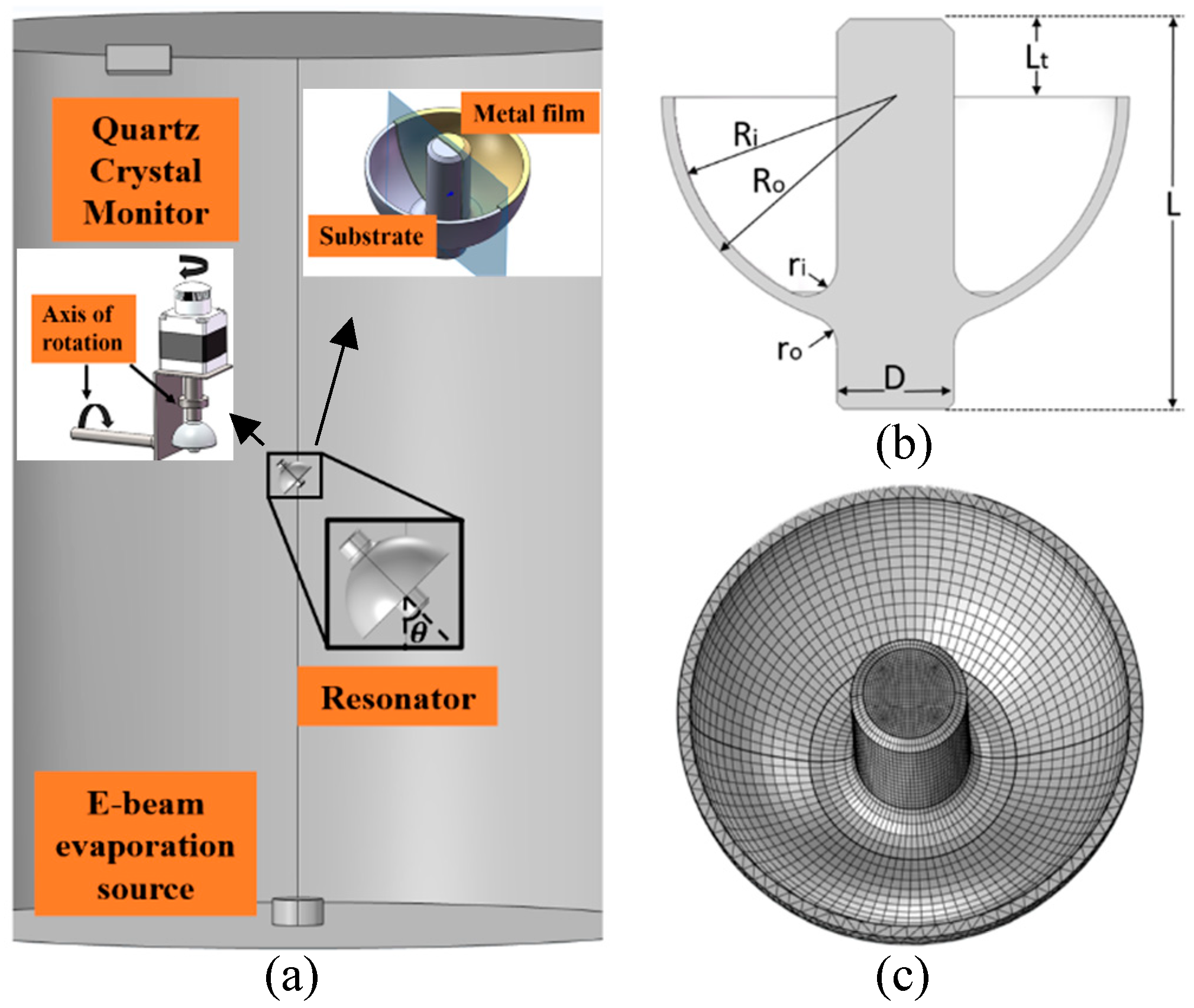
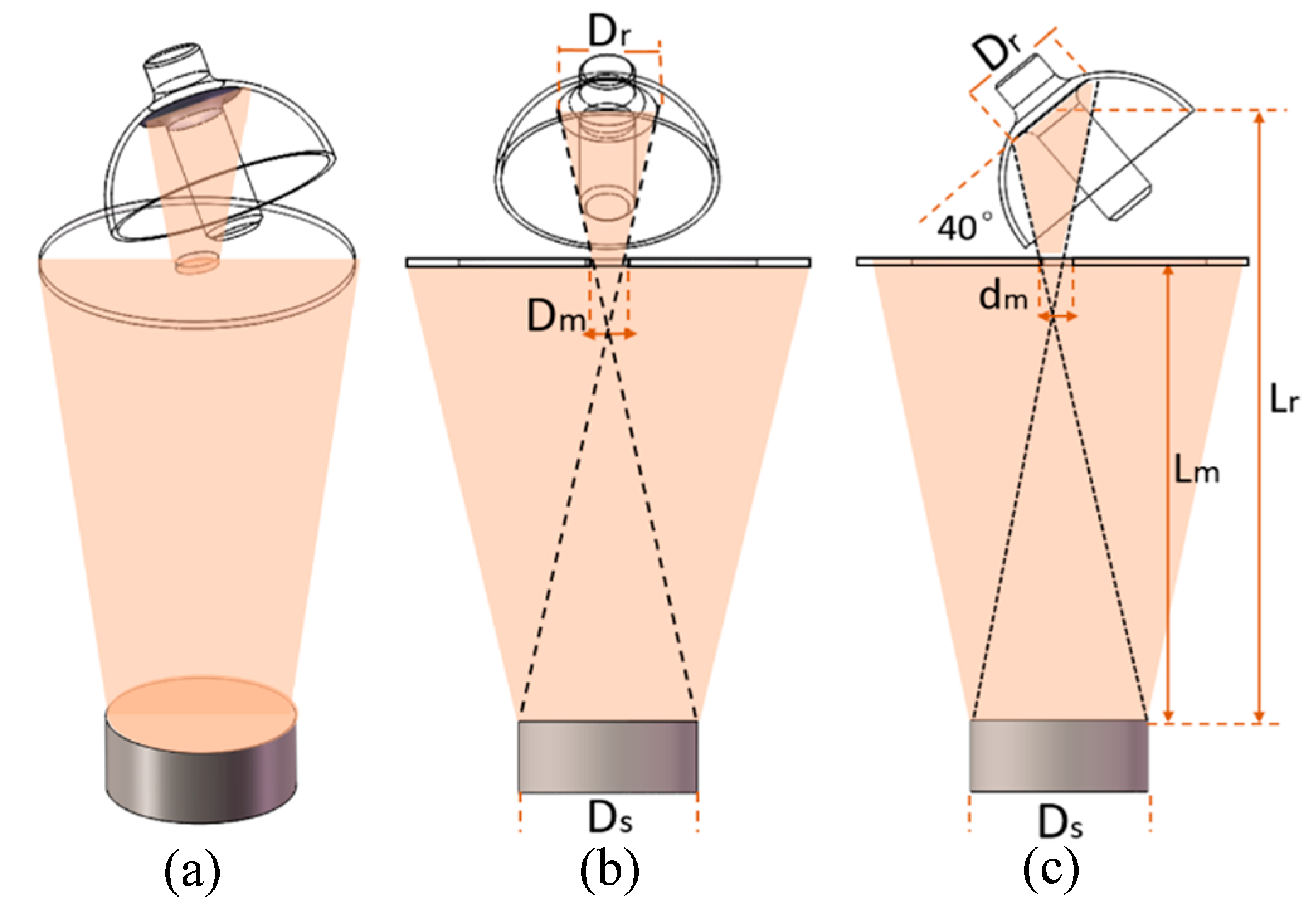
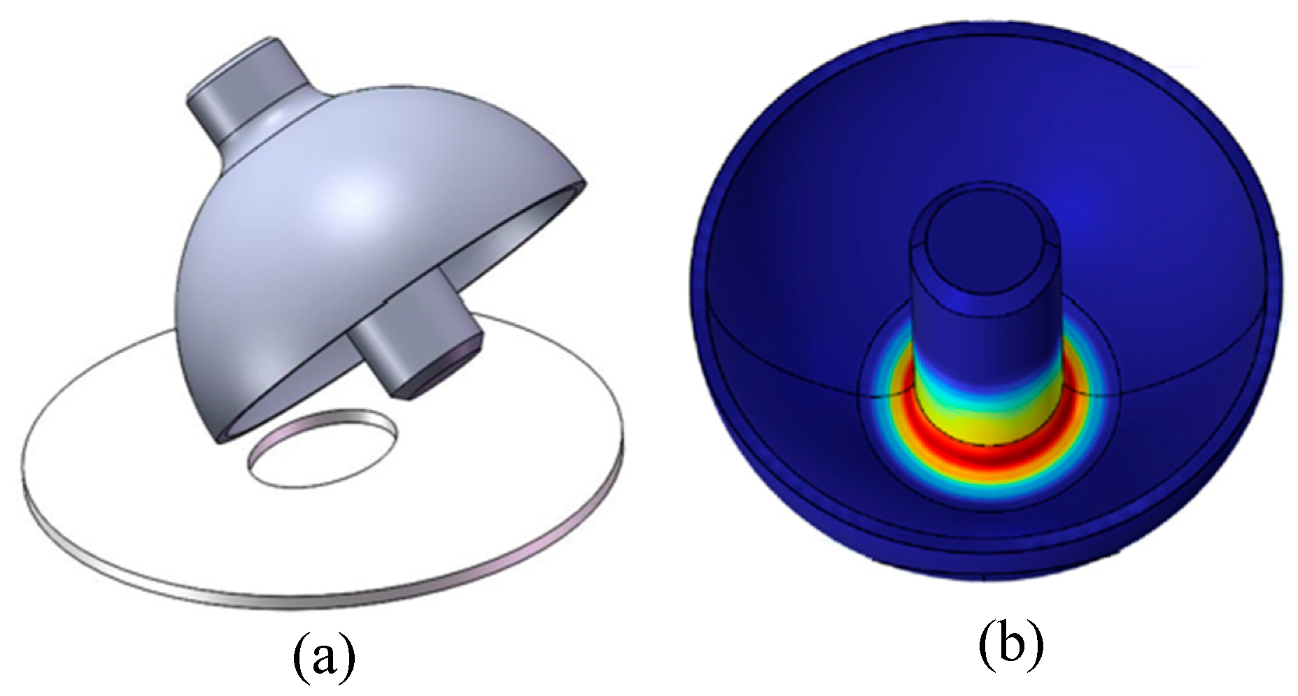
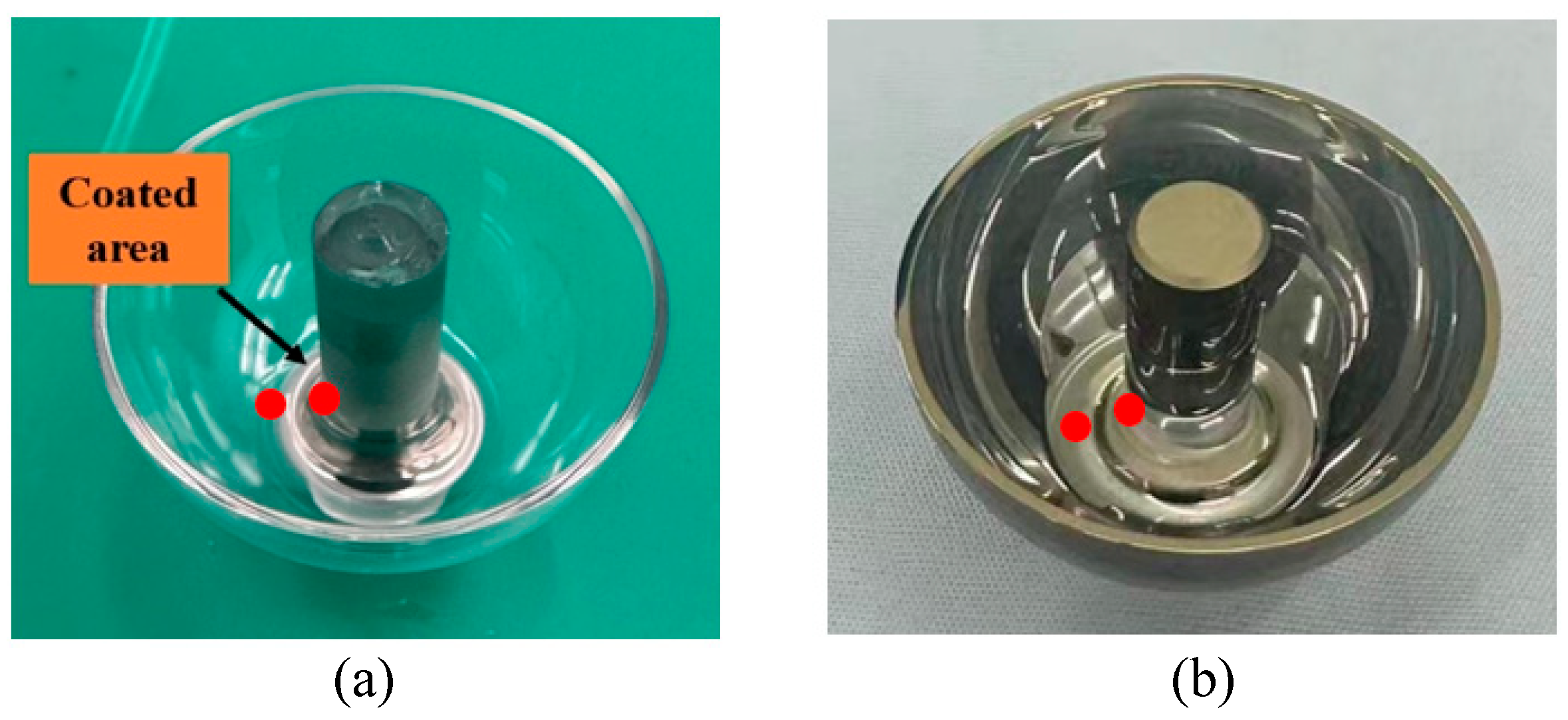
COMSOL Multiphysics is used to numerically solve film deposition problems under the free molecular flow module. The hemispherical resonator is an axisymmetric structure composed of a hemispherical shell and a stem. The junction between the central rod and the shell features a rounded corner transition. The vacuum chamber is a cylindrical structure with a diameter of 300 mm and a height of 1000 mm. The E-beam evaporation source is located directly below the resonator, which is installed 350 mm above it. A Quartz Crystal Monitor (QCM) is installed at the top of the vacuum chamber to monitor changes in the thickness of the deposited film in real time. The resonator is rotatable along two axes, with the inner wall serving as the target region for coating deposition. The axial rotation of the resonator is achieved through a rotating domain with a speed of 4 rad/s. The oscillation of the resonator is defined by the initial deposition angle. In the simulation, the double-layer film structure of the resonator is simplified to a single-layer film, as the material of the film has minimal impact on the uniformity in finite element simulations. This study employs a total of 79,026 meshed elements, with refined meshing applied to the inner wall of the resonator. The spatial distribution of each part is shown in Figure 1a. The parameters and dimensions of the resonator are presented in Figure 1b and

Table 1. The dimensions of a hemispherical resonator.

Parameter Name	Symbol	Dimensions
Inner radius of shell	Ri	14.2 mm
Outer radius of shell	Ro	15 mm
Inner fillet	ri	2 mm
Outer fillet	ro	2 mm
Diameter of stem	D	7.5 mm
Length of stem	L	25 mm
Distance between rim and the end of the stem	Lt	5 mm

, while the meshed resonator is illustrated in Figure 1c.

The material of the hemispherical resonator is fused quartz, and the materials of the film are chromium and gold. To reduce computational complexity, a single-layer chromium film was used for simulation in this paper. In addition, during the simulation process, the resonator is designed to rotate around the stem to ensure the uniformity of the film in the circumferential direction. Coating is a repetitive and accumulative process. Therefore, it is unnecessary to calculate the entire process in detail. This paper presents simulated data demonstrating the distribution of the resonator film thickness when the QCM film thickness reaches 1 nm. It takes 5 s to achieve a thickness of 1 nm, which is close to the actual conditions. These data can be utilized to calculate the trend of film thickness distribution over the entire coating duration.

The coating areas include the inner surface of the shell and the stem. The simulation results indicate that the vast majority of elastic energy (98.65%) is stored in the shell, while only a minimal portion (1.35%) is retained in the stem [21]. Therefore, film thickness uniformity is a critical factor in the region of the shell, because poor uniformity may lead to increased energy losses. The stem region requires a sufficiently thick film to ensure conductivity rather than uniformity.

2.2. Simulation Results

The angle between the central axis of the hemispherical resonator and the evaporation source is denoted as θ, as shown in Figure 1a. When θ = 0°, 10°, 20°, 30°, 40°, 45°, 50°, 60°, 70°, and 80°, the film thickness distribution of the resonator is simulated. Figure 2 illustrates the key characteristics of film deposition at various angles. At an angle of θ = 0°, the highest deposition rate occurs at the inner wall at the center of the hemisphere. This is because the normal direction in this region aligns closely with the deposition direction. In contrast, the peripheral regions of the hemisphere and the stem exhibit minimal deposition, as their orientations are nearly parallel to the deposition direction. As θ increases to 10°, 20°, 30°, 40°, and 45°, the point of maximum deposition shifts from the center of the hemisphere toward the periphery, with effective deposition also appearing on the stems. At angles θ = 50°, 60°, 70°, and 80°, the deposition rate along the inner wall near the periphery exceeds that at the center of the hemisphere. Additionally, a new phenomenon emerges: due to the shielding effect of the spherical shell, the deposition rate at the center of the hemisphere drops to zero.

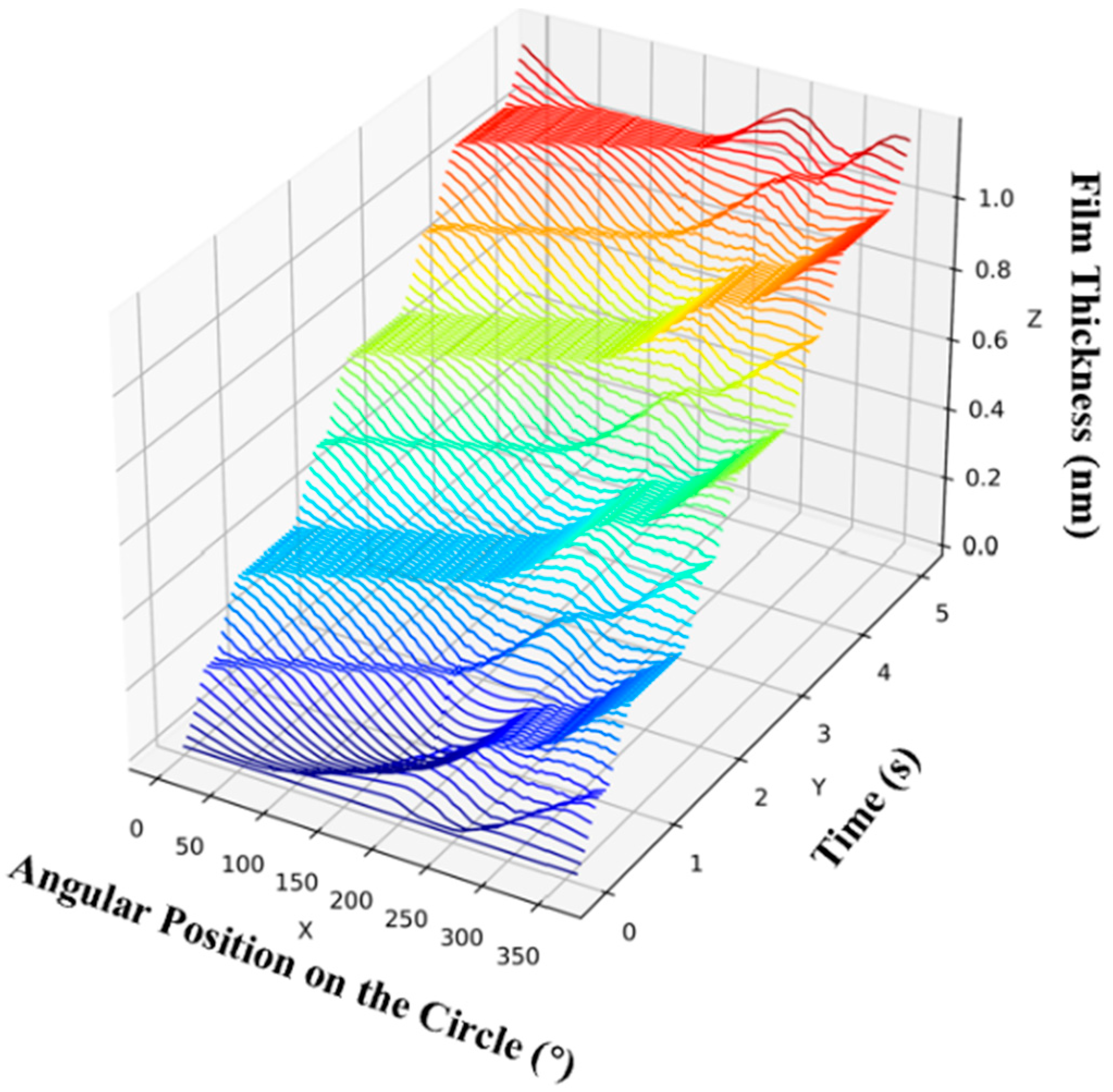
In this study, a systematic analysis of film thickness uniformity in the circumferential direction of the resonator was initially conducted, exploring the effects of deposition angle, circumferential position, and deposition time on film thickness uniformity in this direction. The film thickness distribution along the circumferential direction in the middle of the inner shell from 0 to 5 s at angle θ = 45° is illustrated in Figure 3 and Figure 4. 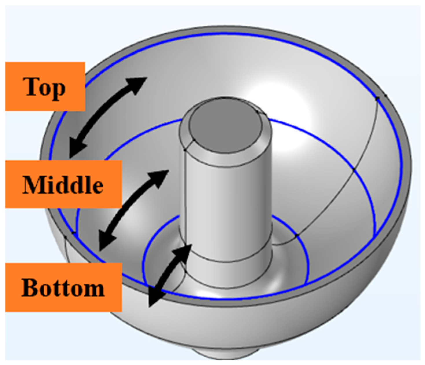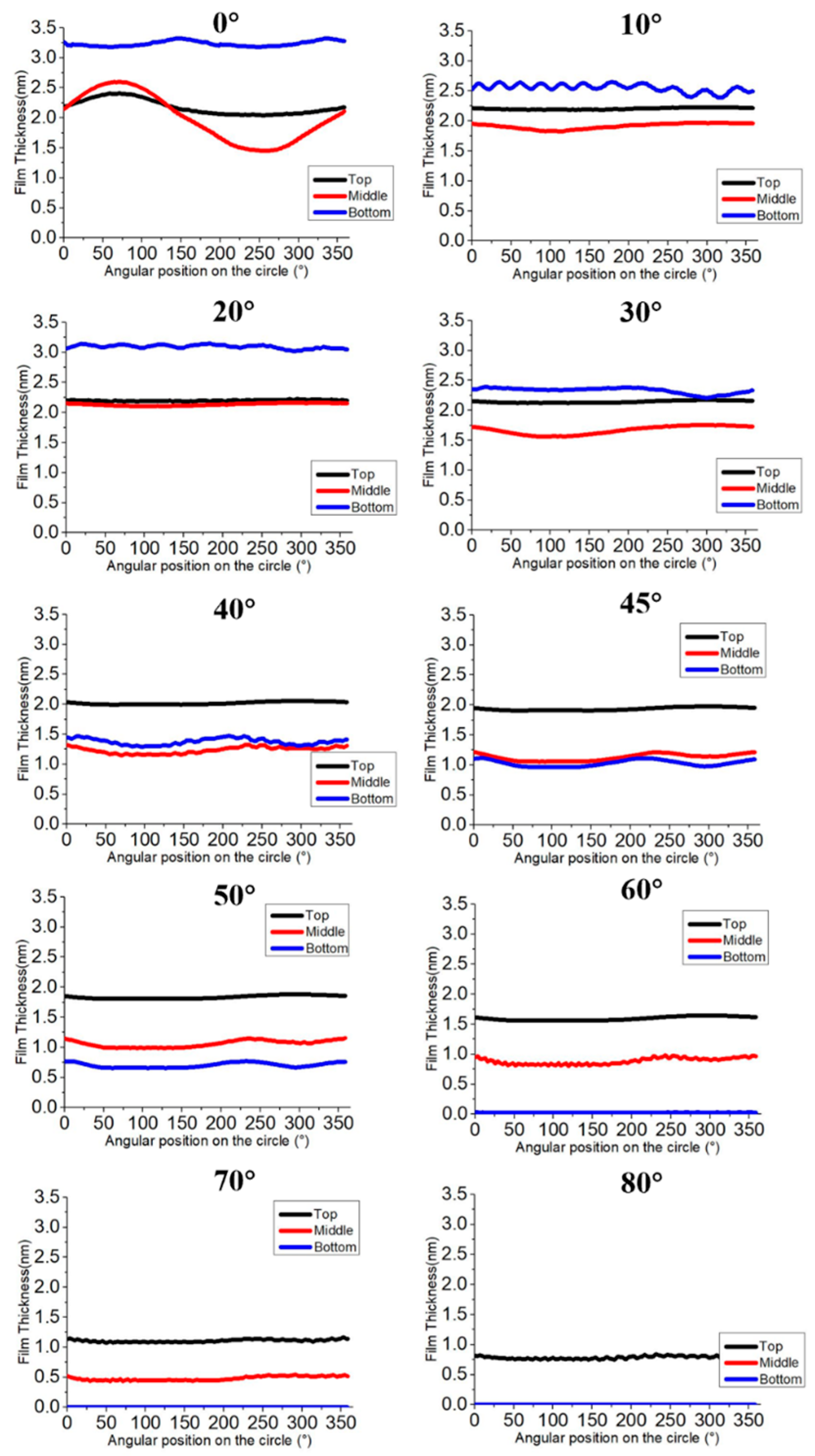The X-axis in Figure 3 represents the angular position along the circumferential direction. The results show that the film thickness at various points along the circumference increases sequentially as the resonator rotates. After one full rotation of the resonator, the peak-and-valley (PV) values of the film thickness remain below 0.5 nm throughout the subsequent deposition process, leading to the conclusion that the uniformity of circumferential film thickness does not worsen with increasing film thickness. On the contrary, it improves as the average film thickness increases. Further analysis shows the distribution of film thickness at the bottom, middle, and top of the shell at 5 s intervals under different deposition angles, as shown in Figure 4 and Figure 5. Under varying angles and positions, the peak-to-valley value of the film thickness does not exceed 1.5 nm. Based on the previous analysis, it is evident that the PV values of the circumferential film thickness are largely unaffected by deposition time. Therefore, when the target film thickness reaches 100 nm, the uniformity of the circumferential film thickness can be maintained and is within an acceptable precision.

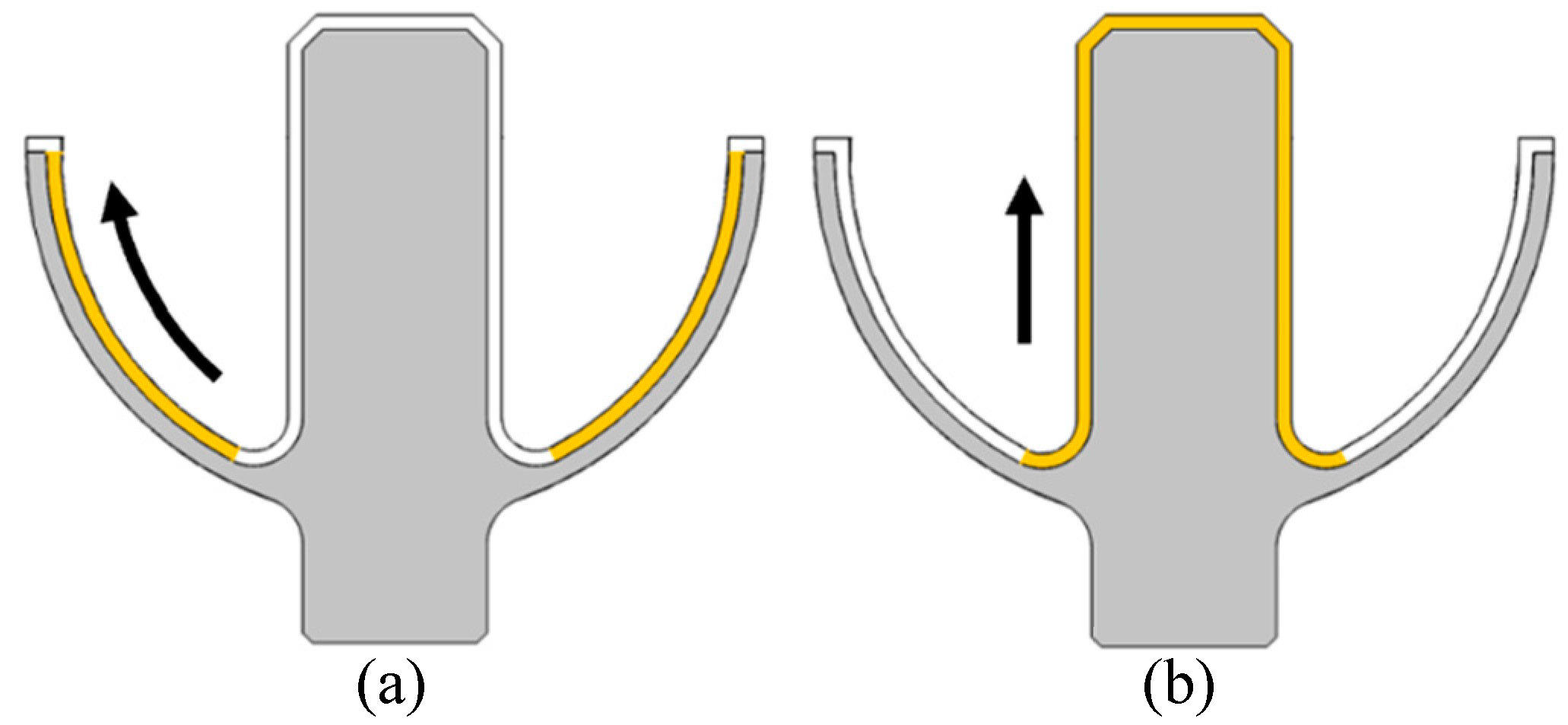
Next, film thickness uniformity was analyzed in the meridional direction of the resonator. Based on the results, it was assumed that the uniformity of film thickness is consistent across any meridian. An arbitrary meridian line was chosen to demonstrate the film thickness distribution from 0 to 5 s; the results are shown in Figure 6. The X-axis represents the position (in mm) in the inner wall along the meridian and the direction shown in Figure 7a. Due to differences in the deposition rate at different positions, the film thickness growth rate is non-uniform. Consequently, the PV values along the meridian line increase as the deposition time increases. Finally, the thickness distribution in the meridional direction at 5 s intervals under various deposition angles is presented. 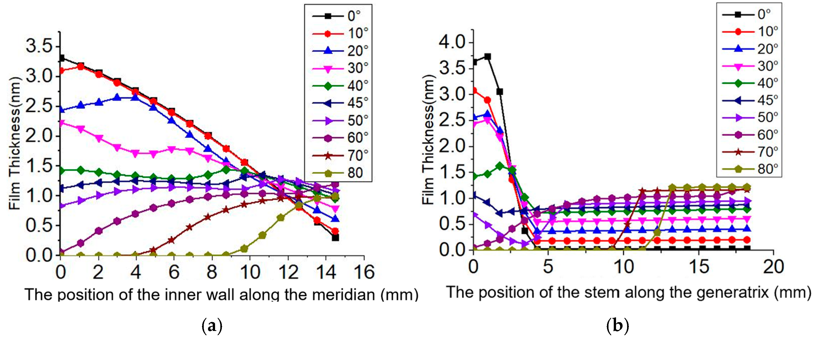Figure 7 illustrates the distribution direction of film thickness, while Figure 8a,b show the film thickness distribution on the shell and stem after 5 s of deposition under different deposition angles, respectively. The X-axis of Figure 8a is the same as the X-axis in Figure 6. The X-axis of Figure 8b represents the position (in mm) in the stem along the generatrix, and the direction shown in Figure 7b. Both Y-axes indicate the film thickness (in nm). These data can be used to calculate the uniformity of film thickness along the meridional direction after the target film thickness has been reached.

Based on the above simulation, the film thickness uniformity on the shell is calculated when the QCM reading is 100 nm. The formula for calculating the film thickness uniformity is

$$∆d=\left({\displaystyle \raisebox{1ex}{$d_{max}-d_{min}$}\!\left/ \!\raisebox{-1ex}{$\overline{d}$}\right.}\right)\times 100\mathrm{\%}$$

(3)

where $d_{max}$ and $d_{min}$ are the maximum and minimum film thickness, respectively, and $\overline{d}$ is the average film thickness.

The film thickness uniformity at all angles is presented in

Table 2. Film thickness uniformity at different deposition angles.

UNIFORMITY
Angle θ(°)	0°	10°	20°	30°	40°
Uniformity	150.1%	139.0%	112.7%	91.8%	37.3%
Angle θ(°)	45°	50°	60°	70°	80°
Uniformity	26.5%	40.1%	139.4%	197.4%	408.7%

. Although the uniformity at coating angles of 40° and 45° is better than that at other angles, it is still not sufficiently optimal. Consequently, the film layer does not exhibit good uniformity on the inner shell of the resonator when using a single deposition angle.

Inducing axial oscillation in the resonator during the coating process may be a potential method to improve the uniformity of the film. Axial oscillation simulation results can essentially be equated to the superposition of thickness distributions at all the angles, including 10°, 20°, 30°, 40°, 50°, 60°, 70°, and 80°, but excluding 45°. Since the simulated film thickness corresponds to a QCM reading of 1 nm, to achieve the actual target thickness of 100 nm, the simulated thickness distribution needs to be superposed 100 times. Under uniform oscillation conditions, these 100 superpositions are equally distributed according to the angular positions obtained from the simulation. The result of film thickness distribution is shown in Figure 9 and the PV value is 60.4 nm. The X-axis of Figure 9 is the same as the X-axis in Figure 8a. Analysis of the results indicates that this method cannot enhance the uniformity of film thickness; thus, it is essential to explore optimized coating strategies. This paper utilizes Proximal Policy Optimization from reinforcement learning to optimize the coating process. The algorithm is integrated with finite element simulation data to enhance the axial uniformity of the film layer.

2.3. Optimization Algorithm

Proximal Policy Optimization (PPO) is a reinforcement learning (RL) algorithm for training an intelligent agent’s decision function to accomplish difficult tasks. When PPO is applied to discrete action spaces, the policy network it uses is typically a neural network that outputs a probability distribution over all possible actions. Specifically, in a discrete action space, PPO selects an action at each time step based on the current policy, with the action sampled according to the probability distribution generated by the policy network. The core idea of the algorithm is updating the policy through gradient descent, increasing the probability of selecting actions that yield higher rewards, thereby gradually improving the overall performance of the agent [22,23,24]. The PPO algorithm demonstrates distinct advantages over other optimization methods. Unlike genetic algorithms (GAs) that rely on random crossover/mutation operations—which may disrupt high-performance sequences—PPO strategically prioritizes exploration in high-reward regions. Compared with grid search methods, PPO avoids the prohibitive computational costs associated with fine-grained angle and timestep discretization in high-dimensional spaces. Crucially, PPO’s inherent suitability for continuous, high-dimensional, and dynamically interactive environments makes it the optimal choice for future multi-degree-of-freedom system development. This includes enhancements such as integrating Planetary Rotation Systems and improving yaw-angle precision—capabilities where GAs fundamentally underperform. The advantages of these algorithms indicate that PPO is a superior choice for coating optimization [25,26].

The PPO model was implemented in Python, utilizing PyCharm Community Edition 2024.2.2 as the development platform, to address the coating problem. The coating process can be divided into discrete time intervals, with each interval corresponding to a 1 nm increase in thickness, as detected by the QCM. The total film thickness on the resonator is obtained by summing the incremental thickness values for each time interval. The film thickness and its distribution at various coating angles have been determined through finite element simulations. To achieve a target film thickness of 100 nm, the process is discretized into 100 steps. In each step, the accumulated film thickness and distribution for a given angle are updated. The entire coating process is simulated by performing 100 iterations, with the PPO algorithm used to optimize the film thickness and distribution at each step. The goal is to minimize the PV value of the accumulated film distribution over these 100 steps. The optimal coating strategy is derived from the output of the selections made at each step.

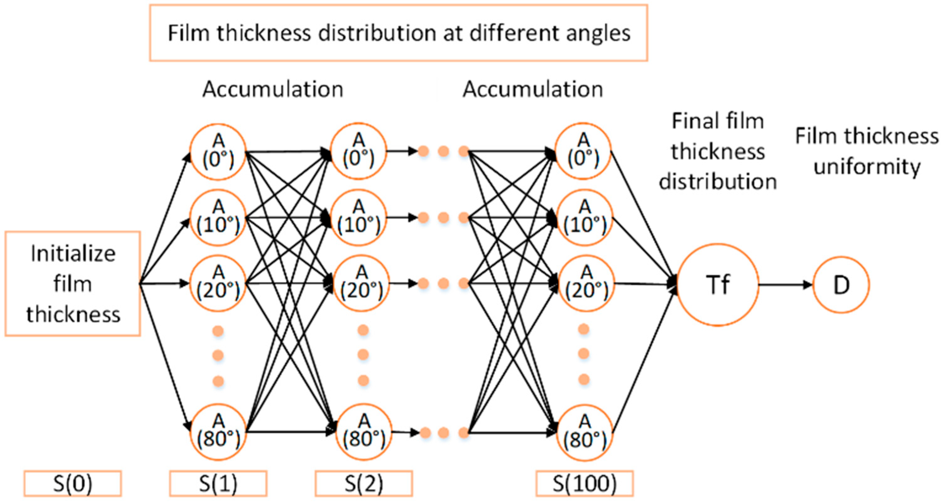
For the task discussed in this paper, it is necessary to define the state and action spaces, in addition to designing the reward function. The “state” represents all the observational information about the environment available to the agent. In this task, the initial state is defined as a film thickness of zero. After each action taken by the agent—selecting a film thickness distribution at a particular angle—the agent observes the accumulated film thickness at the next time step, denoted as S(t). The “action” refers to the agent’s decision based on the current state. Specifically, the agent selects one of ten possible thickness distributions from different perspectives for the subsequent cumulative calculation, as shown in Figure 10. The agent selects a thickness distribution from the ten available options by sampling from the probability distribution output by the Actor network. During training, this sampling encourages exploration, while during evaluation, the highest-probability action is chosen. The probabilities are optimized via PPO’s clipped objective to maximize the reward function (Equation (4)), which penalizes peak-to-valley variations. No explicit cost function is used; the selection is learned end-to-end through policy gradients. In addition, the PPO model ensures escape from suboptimal solutions by continuously exploring the action space during training, while its stochastic policy updates facilitate progressive convergence toward the global minimum, thereby inherently avoiding local minima.

The reward is a scalar value provided by the environment to assess the quality of the actions. The goal of this task is to minimize the difference between the maximum and minimum values of the accumulated film thickness. The reward function is designed to simultaneously minimize peak-to-valley thickness variation while maintaining a reasonable average thickness. Therefore, the reward function is defined as follows:

$$\mathrm{R}\mathrm{e}\mathrm{w}\mathrm{a}\mathrm{r}\mathrm{d}={\displaystyle \raisebox{1ex}{${\mathrm{V}}_{max}+{\mathrm{V}}_{min}$}\!\left/ \!\raisebox{-1ex}{${\mathrm{V}}_{max}-{\mathrm{V}}_{min}$}\right.}$$

(4)

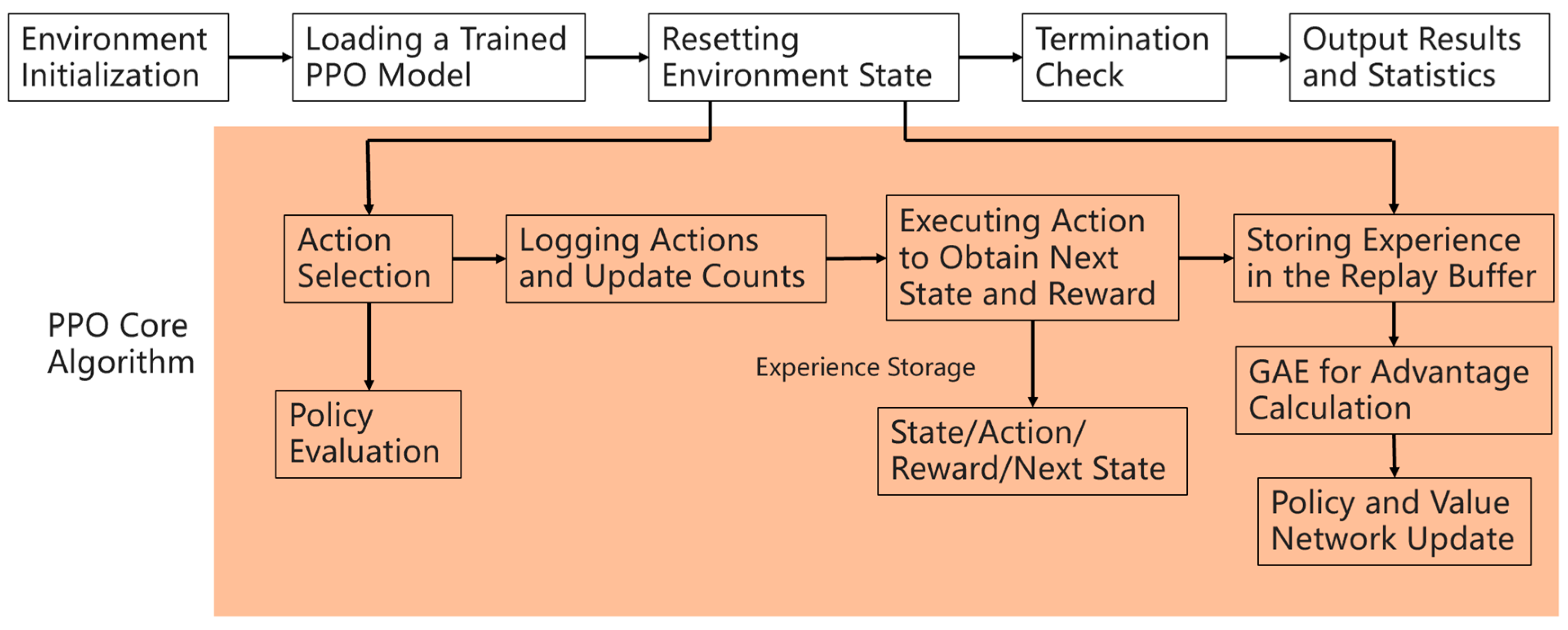
The training process of the algorithm consists of data collection and policy optimization. For data collection, during each episode, the agent selects coating angles based on the current policy. The environment then performs accumulation and returns the new state and reward. The experience tuples (state, action, reward, next state, done) are stored in the replay buffer. For policy optimization, at the end of each episode, the learn method is invoked to compute the Generalized Advantage Estimation (GAE), normalize the rewards, and update the policy network using the Clipped Surrogate Objective to ensure the update magnitude does not exceed ε. Additionally, the Critic network is updated by minimizing the value function error (MSE). The process terminates once the maximum accumulation count is reached [27]. As shown in Figure 11, the core algorithm flow of PPO is illustrated.

Table 3. Key parameters of the PPO algorithm.

Parameter	Value	Description
Learning rate	Actor: 2 × 10−5 Critic: 1 × 10−4	Adam optimizer
Discount factor (γ)	0.99	For long-term reward accumulation
GAE parameter (λ)	0.95	Balance bias-variance tradeoff
Batch size	64	Mini-batch for policy updates
Epochs per update	10	Optimization iterations per batch
Clip parameter (ε)	0.2	Policy updates constraint
Entropy coefficient	0.01	Encourage exploration

presents the key parameters of the PPO algorithm along with their descriptions.

The algorithm incorporates a dynamic masking mechanism that prevents local overfitting by tracking array usage frequency. It employs a dual-save strategy, preserving both the best-performing and final models to optimize exploration-exploitation balance. Additionally, real-time TensorBoard monitoring tracks Actor/Critic losses, reward trends, and state differences.

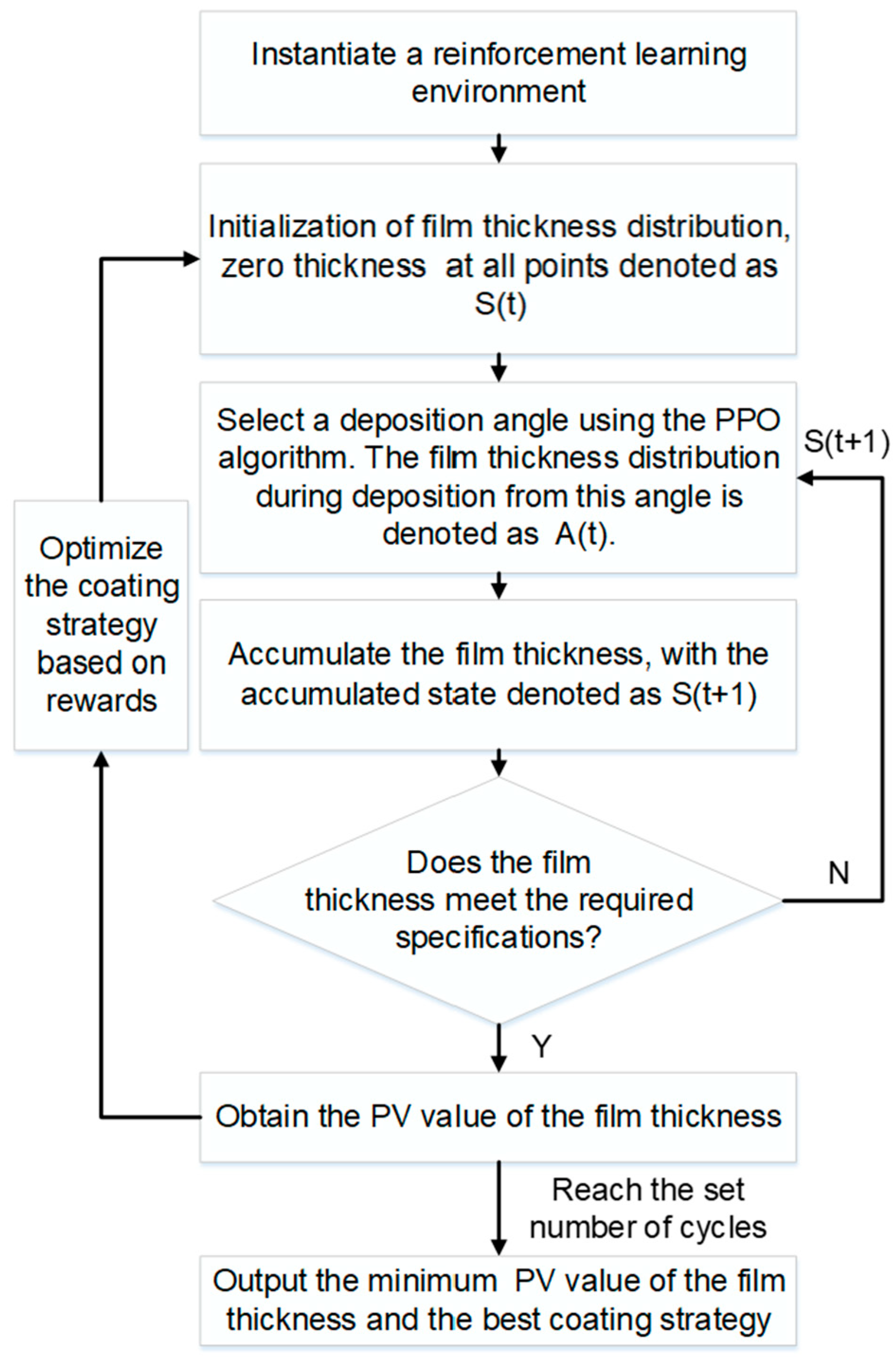
The model was then trained multiple times, and the trained model was subsequently employed to process the simulation data in an iterative optimization framework. During the computational procedure, 1000 optimization cycles were executed to identify the optimal coating strategy. Figure 12 shows the flowchart of PPO for the coating process. During each iteration, the model outputs the PV value of the film thickness under the current strategy. After 1000 iterations, the model identifies the iteration with the minimum PV value and provides the corresponding deposition time required for each coating angle under that strategy. 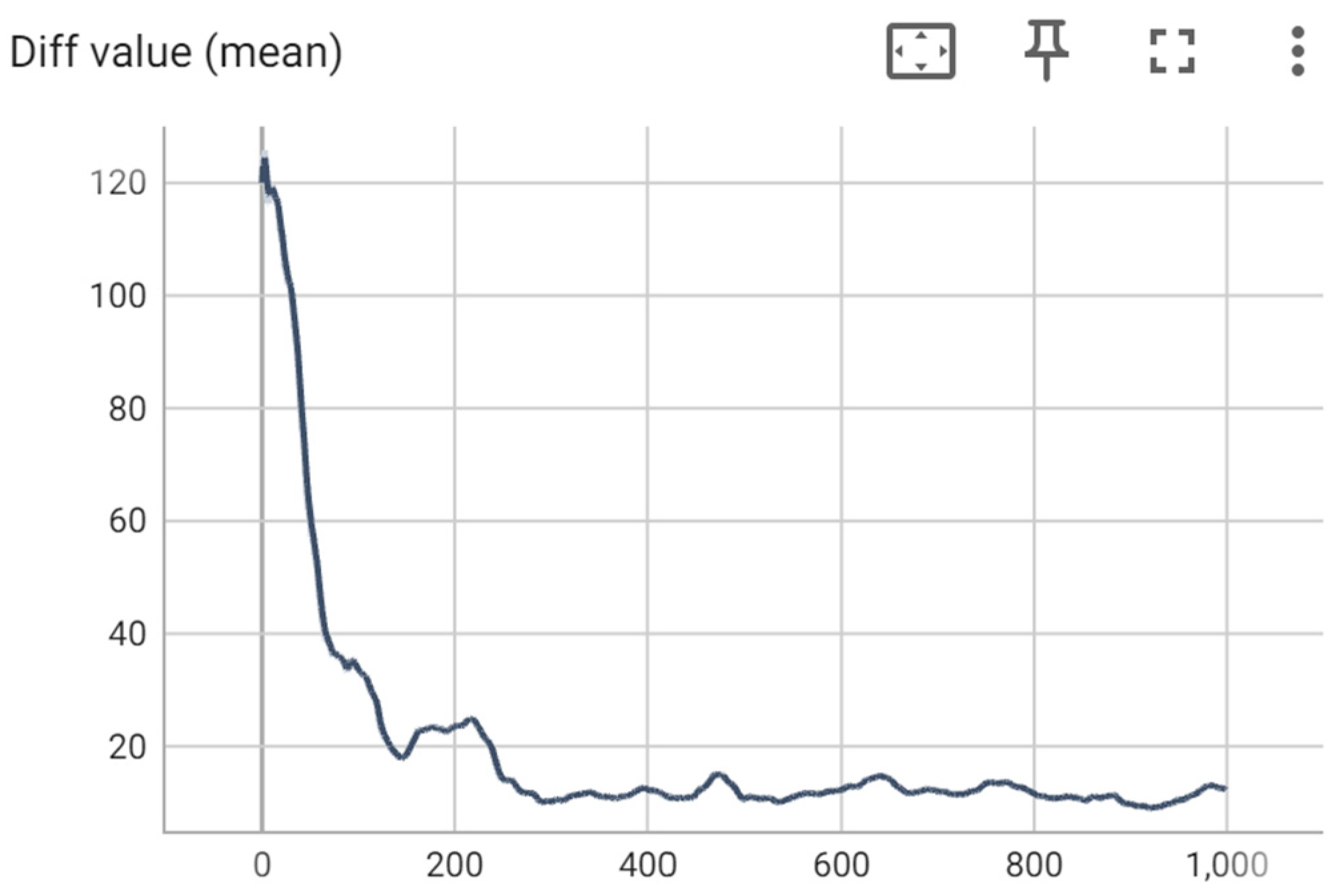Figure 13 illustrates the PV value output during each of the 1000 iterations. After approximately 250 iterations, the PV values consistently remain below 15 nm, indicating good convergence of the model’s algorithm. This suggests that the model is well-suited for optimizing coating strategies and can be effectively applied to optimize the coating process of resonators with varying requirements and dimensions in further applications.

Table 4. The deposition time at different angles.

Deposition Time
Angle(°)	0°	10°	20°	30°	40°
Time	0	0	0	32	11
Angle(°)	45°	50°	60°	70°	80°
Time	10	3	18	0	27

presents the results obtained from the PPO output, showing the deposition angle and the corresponding time required for each angle. The unit of time is the time required for the QCM reading to increase by 1 nm. Since the rate of increase in the QCM reading is influenced by various deposition parameters, which are subject to continuous optimization during the coating process, the exact times are not specified in this study. Instead, the QCM reading is used as a reference for time. Since the target film thickness is 100 nm, the calculation is completed when the film thickness recorded by the QCM reaches this value.

Therefore, based on the data from Table 4 output by the PPO algorithm, the actual coating process is performed as follows: Initial deposition begins at a deposition angle of 30° until the QCM indicates a film thickness of 32 nm. The deposition angle is then adjusted to 40°, and deposition continues until the QCM-measured thickness increases by an additional 11 nm. Subsequently, the deposition angle is further increased to 45°, and the process repeats in this stepwise manner. By following this protocol, a highly uniform film can be achieved on the inner surface of the resonator.

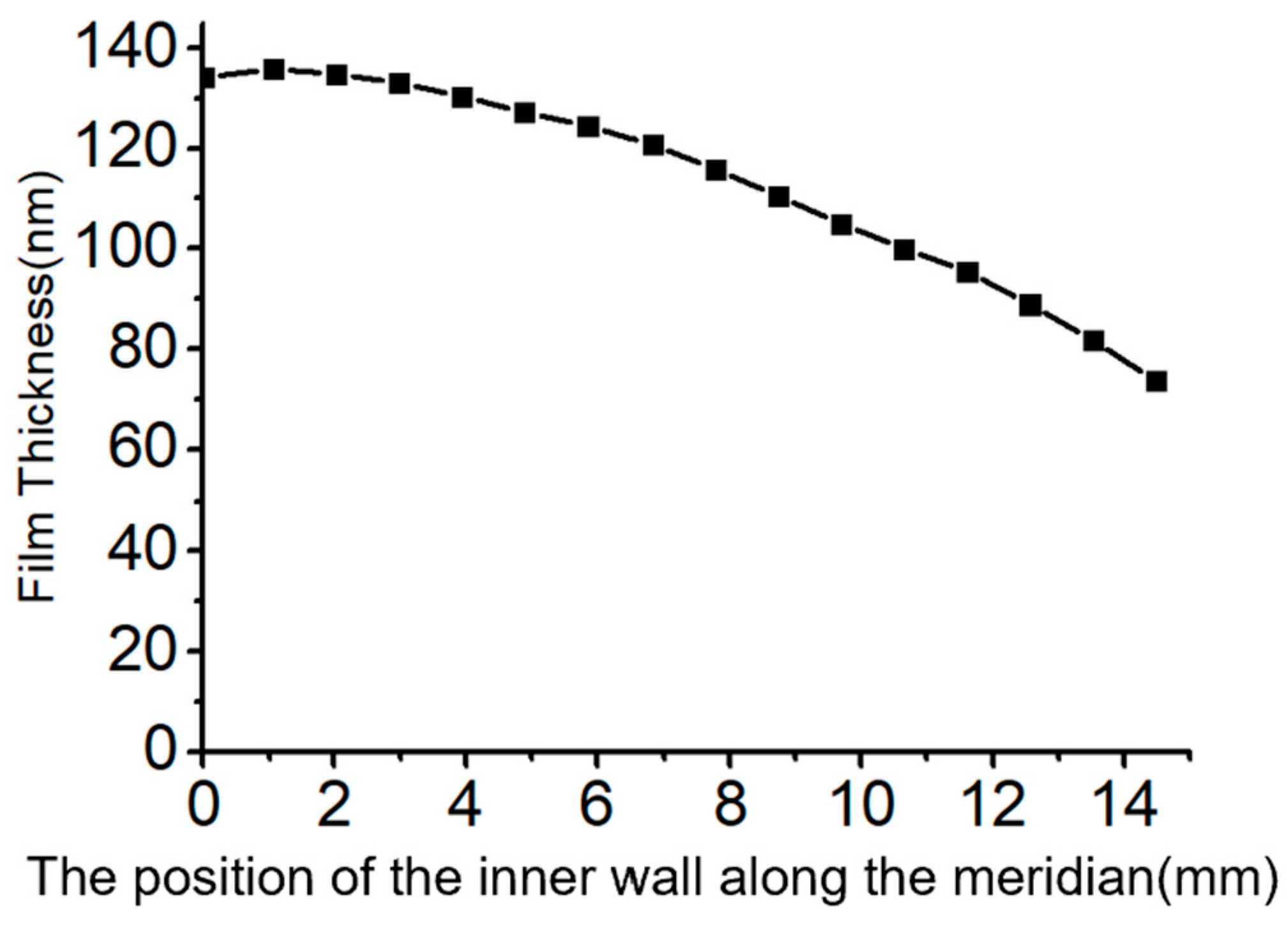
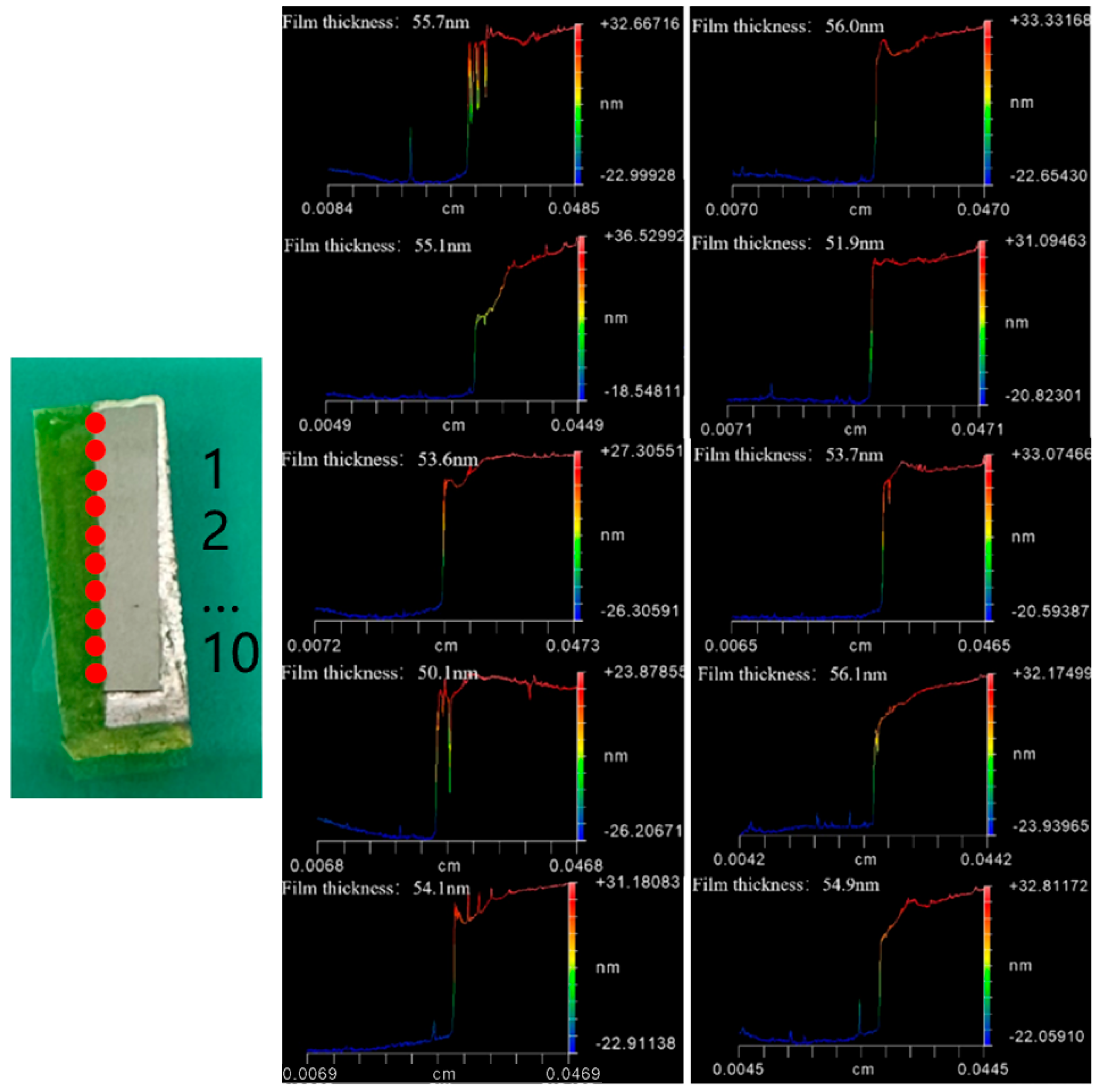
Figure 14 presents the thickness distribution of the shell and stem obtained through COMSOL using the optimized coating process. The X-axis denotes the position (in mm) in the inner wall along the meridian, extending from the edge of the shell, passing through the junction, to the stem termination. The Y-axis represents the deposited film thickness (in nm). The film thickness data in the shell section are as follows (in nanometers): 98.33, 102.25, 103.61, 103.51, 101.51, 99.26, 98.68, 100.65, 103.37, 103.16, 99.45, 98.31, 99.38, 101.36, 102.47, 101.99. The film thickness uniformity was determined to be 5.24% according to Equation (3). This result demonstrates the effectiveness of the finite element method combined with reinforcement learning algorithms in improving film uniformity. However, as shown in Figure 15, another key issue arises: while the optimized process improves the film uniformity on the shell, it results in thinner films in other areas, which lead to an increase in the resistance of the entire hemispherical resonator. The film thickness data in the junction and stem are as follows (in nanometers): 103.21, 71.95, 74.11, 75.56, 107.23, 109.36, 99.52, 83.68, 58.76, 46.78, 50.33, 53.24, 54.37, 55.33, 55.95, 56.35, 56.61, 66.52, 90.41. This paper addresses this issue by using a correction mask.

3. Establishing the Correction Mask

The junction between the shell and the rod is a special region where the film deposition rate is lower. This is because, in this area, the film cannot be deposited vertically at arbitrary angles, as the shell and rod create shadowing effects. In addition, the instability of the processing technique and excessive surface roughness can lead to the formation of counter-slopes, which are blind spots for vapor deposition. If counter-slopes are present at the junctions, inadequate deposition can lead to excessively high resistance or even a circuit breaker in hemispherical resonators, as shown in Figure 15. In fact, the upper part of the stem also has areas with thinner film, but the thinner film in this part has little effect on the resonator. This is because when the coating angle is large, the upper region of the stem can be nearly vertically deposited, which is not affected by counter-slopes. Additionally, the stem is easier to process compared to the junction, so counter-slopes are unlikely to occur in this region. Furthermore, this part serves as the support area for the resonator, where conductive solder will be applied to connect with other components. Therefore, this paper does not consider the thin film on the stem but focuses only on the issue of the thin film on the junction.

To address this issue, a correction mask is used to ensure sufficient deposition at the junction, without affecting the uniformity of the film on the shell [28]. After the coating achieves high uniformity on the shell, a correction mask is added. This mask blocks the deposition of coating material onto the shell, allowing the coating material to only be deposited at the junction. Consequently, the correction mask needs to be designed to meet these requirements [29].

Based on the simulations, the deposition rates of the coating at various points along the junction are relatively higher when θ = 40°. Therefore, a correction mask is applied at a coating angle of 40°. The correction mask is designed as a horizontal plate for ease of automated application in the future. Figure 16 illustrates the spatial arrangement among the evaporation source, the correction mask, and the resonator. The dimensions of the correction mask were designed based on spatial geometry.

$$D_m={\displaystyle \raisebox{1ex}{$D_r{L}_r-\left(D_s+D_r\right)\left(L_r-L_m\right)$}\!\left/ \!\raisebox{-1ex}{$L_r$}\right.}$$

(5)

$$d_m={\displaystyle \raisebox{1ex}{$D_{r}cos40°L_r-\left(D_s+D_{r}cos40°\right)(L_r-L_m)$}\!\left/ \!\raisebox{-1ex}{$L_r$}\right.}$$

(6)

where $D_m$ and $d_m$ are the major axis and minor axis of the elliptical hollow, $D_s$ is the diameter of the evaporation source, $D_r$ is the diameter of the junction, $L_r$ is the distance from the evaporation source to the resonator, and $L_m$ is the distance from the evaporation source to the mask. The major axis of the elliptical hollow is 11.5 mm, and the minor axis is 8.5 mm. The designed correction mask is applied in the simulation of the coating process, with the results displayed in Figure 17. After the installation of the correction plate, the film is deposited only at the junction and stem, with no deposition on the shell. The feasibility of the correction mask was confirmed through simulation verification, followed by its production, which to some extent ensured its effectiveness and practicality while saving both time and cost.

4. Experimental Verification

4.1. Experimental Installation

An electron beam evaporator was used for film deposition, with step height profiling applied for thickness measurement on curved substrates. Figure 18a illustrates the dual-axis rotation fixture used for the rotation and fixation of the resonator during the coating process. The specific procedure is as follows: a flexible glass substrate was bent and conformally attached to the inner wall surface of the resonator, as shown in Figure 18b,d, with 50% of the substrate area covered by anti-coating tape prior to thin-film deposition. This ensured the formation of a continuous film layer on the exposed region while maintaining the initial state of the masked region. After deposition, the substrate was removed and restored to its planar state, followed by the removal of the tape, resulting in a well-defined step structure at the film interface.

The step height was quantitatively analyzed using a Zygo white-light interferometric profilometer. The obtained data were processed to effectively characterize the film thickness uniformity along the meridian direction of the resonator’s inner wall [30]. Furthermore, a correction mask was fabricated according to the design specifications, and a supporting device for the correction mask was designed and manufactured to ensure its precise spatial positioning, as shown in Figure 18c.

4.2. Experimental Result

The target film thickness for this experiment was set to 100 nm, and the deposition process was terminated when the QCM reading reached 100 nm. The thickness was measured using the Zygo white-light interferometer shown in Figure 19c. Interference fringe patterns were acquired and processed through phase unwrapping to generate surface profiles at the step regions, as shown in Figure 19a,b. Tilt removal was subsequently applied to these profiles to obtain step height maps for thickness evaluation. The step height at each position is determined by performing line scans across the step edges, with ten measurement points evenly distributed along the steps of the flexible glass, as shown in Figure 20. The experimental results revealed that while the target thickness was 100 nm, the deposited thickness on the resonator’s inner wall using the simulation-optimized process was approximately 50 nm.

Table 5. The film thickness at different locations measured by white light interferometry.

Film Thickness
Measurement position	1	2	3	4	5	6°	7	8	9	10
film thickness (nm)	55.7	56.0	55.1	51.9	53.6	53.7	50.1	56.1	54.1	54.9

presents the measured film thickness values at various measurement locations. Based on the measured thickness data, the uniformity of the film thickness was calculated using Equation (3), yielding a final uniformity of 11%. This deviation from the simulated film thickness uniformity of 5.24% arises because the COMSOL simulation is based on idealized assumptions that may deviate from actual conditions. The simulation assumes particles undergo collision-free, rectilinear motion, neglecting potential scattering effects present in real deposition processes. For instance, during actual deposition, the system is typically heated to approximately 100 °C, which reduces the vacuum level to about 8 × 10⁻⁴ Pa; this affects particle motion to some degree. Furthermore, the electron beam evaporation source in the simulation is idealized, whereas practical equipment exhibits imperfections such as non-uniform crucible thermal fields and beam spot drift. Additionally, the considerable distance (approximately 350 mm) between the resonator and the evaporation source introduces spatial positioning errors that may also impact coating performance. Nevertheless, the coating process was successfully optimized in this study and the uniformity of the inner wall film was significantly improved.

As shown in Figure 21a, the correction mask strategy resulted in localized film deposition exclusively at the interface between the resonator’s stem and shell, with no deposition observed on the spherical shell. Figure 21b shows the resonator without using a correction mask for coating. The resistances at the junction of these two resonators were measured at the locations marked by red dots in the figure, with the region coated using the correction mask exhibiting a resistance of only 0.45 kΩ, while the junction of the resonator without the correction mask showed a resistance of 7 kΩ. This approach effectively enhances the thickness and reduces the resistance at the rod–shell interface while preserving the uniformity of the spherical shell coating.

5. Conclusions

This study focuses on optimizing the uniformity of thin films during the hemispherical resonator coating process. By integrating numerical simulations, optimization algorithms, and experimental validation, we comprehensively investigated the critical factors influencing film uniformity and proposed systematic process improvement strategies.

First, we utilized the free molecular flow module in COMSOL to simulate the coating process under various resonator tilt angles. By precisely calculating the thickness distribution across all tilt angles, we revealed the significant impact of resonator tilt on film uniformity. This numerical simulation-based process analysis provided a theoretical foundation and guidance for optimizing the coating process, significantly enhancing research efficiency. Building on the simulation results, we introduced the Proximal Policy Optimization (PPO) algorithm to intelligently plan the coating process. By training on thickness distribution data under different tilt angles, the PPO algorithm successfully optimized the coating parameters for the resonator, achieving a film uniformity of 5.24%. This demonstrates a novel application of intelligent algorithms in thin-film fabrication processes. Although the PPO-optimized coating process significantly improved film uniformity, localized areas with insufficient thickness remained. To address this issue, we proposed and implemented a masking technique to locally enhance the thickness in these regions. To validate the effectiveness of the optimized process, we conducted experimental tests and used a Zygo white-light interferometer to precisely measure the thickness distribution post-coating. The experimental results confirmed that the optimized process significantly improved the uniformity of the thickness distribution, achieving an actual uniformity of 11.0%. By combining numerical simulations, algorithmic optimization, and experimental validation, this study not only addressed the issue of film uniformity in hemispherical resonator coatings but also established a general method for optimizing coating processes on complex surface structures and batch components. The Finite Element Method enables not only the construction of intricate models but also the simulation of multi-degree-of-freedom motion states, such as a planetary rotation system that incorporates both rotation and revolution of components. The design of corrective masks can also be performed via finite element simulation, where adjusting the mask dimensions allows direct visualization of thickness distribution variations. Relying solely on experimental coating trials to explore process parameters—such as complex geometries, multi-axis motion, and mask shape/size—would be extremely time-consuming. However, pre-simulating these variables through finite element analysis significantly reduces development time. Furthermore, the trained PPO optimization algorithm can be rapidly deployed across diverse operating conditions to enhance coating uniformity, demonstrating its unique advantage in adaptive process control.