A Contribution of XPS and Electrochemistry to the Understanding of Hydrogen Diffusion in X60 Steel

Abstract

Sustainable storage and transport of hydrogen are challenges in the transition to renewable energy sources. Hydrogen embrittlement (HE), caused by atomic hydrogen absorption and diffusion into steel, influences the mechanical properties of steel pipelines and reservoirs. This work focuses on the hydrogen diffusion on X60 pipeline steel using electrochemical measurements and X-ray photoelectron spectroscopy (XPS). The hydrogen permeation tests (HPT) were performed to estimate the effective hydrogen diffusion coefficient D_eff and the subsurface hydrogen concentration C₀ in cleaned and mechanically polished X60 steel. XPS analysis confirmed the presence of a 6 nm thick film of Fe (II) oxide, Fe (III) oxide, and Fe (III) oxyhydroxide. Mechanical polishing improved oxide layer uniformity, ensuring reproducible electrochemical behavior. The effective hydrogen diffusion coefficient D_eff was determined for X60 steel using t_lag and t_b methods. It was found in the range from 2.0 (0.4) 10⁻¹⁰ m²/s to 2.9 (0.5) 10⁻¹⁰ m²/s. The subsurface hydrogen concentration, C₀, was found to be 0.7 (0.1) ppm for X60 steel. The hydrogen diffusion in X60 steel depends on its bulk properties; it is unaffected by surface preparation methods, and it is confirmed to be lower than in high-carbon and other high-strength steels.

1. Introduction

One of the main problems of sustainable energy production is the discrepancy between electricity production and electricity consumption [1]. Typical examples are the high production of electricity by solar cells in the summer and the demand for electricity in the winter. Therefore, solutions are needed to store renewable energy from summer to winter. As electrical energy cannot be stored in sufficiently high quantities in batteries, other seasonal energy storage solutions have to be found. One frequently used way to store electrical energy is electrolysis, which produces “green hydrogen” (hydrogen produced by sustainable energy sources) from cheap or even excess solar power in the summer and uses it to generate electricity in the winter. Efforts are underway to address the challenges associated with the efficient storage and transport of hydrogen; the traditional way to store hydrogen both in liquid form at cryogenic temperatures and as pressurized hydrogen gas in tanks is expensive and not very efficient. Different ways of storage are proposed in the literature; researchers propose a chemical storage way, relying on the steam-iron process [1]; an alternative to seasonal energy storage is “power to aluminum” [2]. Excess electrical current is used to reduce aluminum hydroxide to elemental aluminum; during the reverse process, Al is oxidized to aluminum oxide or hydroxide, and hydrogen gas and heat are released.

For hydrogen transport over longer distances, steel pipelines are the favored choice due to their lower cost, high efficiency, and safety [3,4]. However, atomic hydrogen can absorb and diffuse into steel and potentially degrade its mechanical properties; this phenomenon is known as hydrogen embrittlement (HE) [5,6]. A laboratory study showed that hydrogen accelerated the fatigue of API X60 pipeline steel and its welds; it was found that hydrogen accelerated the crack growth phase in API X60 steel by a factor of 8 [7], which might seriously reduce the time of operation of the pipelines. The stress corrosion cracking (SCC) susceptibility of X60 steel was studied with slow strain rate tests in a solution simulating groundwater; it was found that the failure process was controlled by hydrogen embrittlement and anodic dissolution [8]. When repurposing existing gas pipelines for blended hydrogen or pure hydrogen transport, the hydrogen embrittlement sensitivity of the steels used has to be evaluated. Hydrogen embrittlement of X60 steel became more severe in 100% pure hydrogen, and the formation of secondary cracks was observed [9]. Hydrogen induced cracking susceptibility of X60 steel was studied, and the tensile test results showed that the ductility dropped by 83% in the hydrogen-charging environment [10].

Hydrogen embrittlement affects the performance of the steel pipelines, resulting in material degradation that leads to hydrogen leakage, which can cause combustion and possible explosion due to the wide range of flammability of hydrogen [11,12]. In addition, HE impacts the reliability and safety of metal structures in several other industries, such as aerospace, automotive, and construction [13], with possibly catastrophic consequences, especially in energy facilities such as power plants and nuclear plants [14].

For this reason, further investigations on materials are required for safely transporting hydrogen gas via steel pipelines. Key factors influencing HE are the diffusion behavior of absorbed atomic hydrogen within the material and its impact on the cohesive forces within the steel’s crystal lattice [5]. The HE mechanism is mainly determined by the interaction between the absorbed hydrogen and the traps, such as grain boundaries, dislocations, and vacancies [6].

Techniques for investigating hydrogen diffusion in steel are essential. The electrochemical permeation test is performed using a Devanathan–Stachurski cell [15], which is a powerful electrochemical technique that provides information not only on the diffusion coefficient but also on the trapping of hydrogen in steel [16]. It consists of two electrochemical cells, the hydrogen production and the detection cells, separated by the sample clamped in between (working electrode: WE). In this study, an analytical approach based on in-situ techniques, such as the hydrogen permeation test (HPT), and surface analytical ex-situ techniques, X-ray photoelectron spectroscopy (XPS), was used on cleaned and mechanically polished X60 steels to clarify whether different surface treatments influence the hydrogen permeation results. HPT was also utilized to determine the effective diffusion coefficient and the subsurface concentration of hydrogen in steel. This work aims to develop an analytical method and investigate the hydrogen permeation in X60 pipeline steel to estimate the effective diffusion coefficient and the hydrogen subsurface concentration. The results of this work are the basis for future studies on X60 steel with hydrogen permeation barrier (HPB) coatings.

2. Materials and Methods

2.1. Materials

The steel studied in this work is API 5L X60QS steel. API 5L is the standard specification of the American Petroleum Institute for seamless and welded pipelines. The pipelines are made of carbon steel pipes used for oil and natural gas transportation. The abbreviation “X60” defines the minimum yield strength (60′000 psi or 415 MPa). This (high) strength is achieved through the addition of alloying elements such as manganese, silicon, and chromium. The steels “X65”, “X70”, and “X80” have a higher yield strength. Q refers to the production process, such as R: as rolled, N: normalized, Q: quenched and tempered, M: thermomechanical rolled, whereas S refers to the sour service use. The X60 steel samples were cut from a section of an as-produced carbon steel API 5L X60QS seamless pipe. According to API specifications [17], the chemical composition of an API 5L X60Q steel is reported in Annex H, paragraph H.4.1, table H1, page 126.

The diameter and thickness of the disk samples were 50 mm and 2 mm, respectively. The bulk composition of the X60 steel sample determined by portable X-ray fluorescence spectroscopy is provided in

Table 1. Bulk composition (mean values, wt.%) of X60 steel determined by portable X-ray fluorescence spectroscopy. Standard deviations are in parentheses. P and S are below the limits of detection (LoD) of the p-XRF.

	Fe	Mn	Cr	Mo	Ni	Cu	S	P
Wt.%	98.2 (0.1)	1.20 (0.04)	0.20 (0.02)	0.10 (0.01)	0.10 (0.01)	0.10 (0.01)	<LoD	<LoD

. P and S are below the limits of detection (LoD) of the pXRF. The instrument used was the hand-held SPECTRO xSORT (Spectro Analytical Instruments GmbH, Kleve, Germany); the analysis conditions were suggested by the supplier for the method named “precious metals” [18].

It is noteworthy that all elements were found to be below the maximum concentration specified for an API 5L steel. The concentration of C could not be revealed by X-ray fluorescence spectroscopy.

The metallographic examinations of the cross-section of X60QS steel (etched with 2% Nital solution for 5 s) revealed an irregular grain size and shape with globular carbides along the grain boundaries, thus confirming a bainite/martensite microstructure as expected on a quenched and tempered product (Figure S1).

2.2. Sample Preparation

After cutting, the “as received” X60 steel was covered with an oil/grease film. Two different procedures were adopted for the surface preparation on both sides of the X60 steel disks:

• Procedure 1: Five solvent cleaning.

The as-received samples were covered with grease from the cutting process. They were cleaned in an ultrasonic bath at 40 °C using five solvents for 5 min each: butan-2-one (purity > 99.5% (CAS Nr. 78-93-3) purchased from Chem-lab, Zedelgem, Belgium), acetone ≥ 95.5% (CAS Nr. 67-64-1), ethanol absolute ≥ 99.8% (CAS Nr. 64-17-5, purchased from Honeywell, Offenbach, Germany), petroleum ether (CAS Nr. 650-001-01, purchased from Carlo Erba Reagents S.r.l, Cornaredo, (MI) Italy), and double distilled water (specific conductivity equal to 1.5 (0.1) μS/cm). Organic solvents were used to reduce the carbon signal, C1s, present on the sample surface. A polar solvent, double-distilled water, was used to remove the deposits of inorganic salts (e.g., Ca²⁺, Zn²⁺). The XP-spectra was obtained after washing the sample with each solvent to monitor the removal of the organic compounds. This protocol was established in this work to achieve reproducible electrochemical measurements.

• Procedure 2: Five solvents cleaning and mechanical polishing

The samples were cleaned with five solvents as described above and mechanically polished using 4000-mesh SiC paper (Struers, Ballerup (DK)) and ethanol as lubricant for three minutes and thirty seconds. After mechanical polishing, the samples were immersed in an ultrasonic bath at 40 °C in ethanol for five minutes and in double-distilled water for ten minutes.

Following the cleaning and/or the mechanical polishing, the disks were heated at 80 °C for 15 h to remove any hydrogen that might be trapped in the steel following the manufacturing.

2.3. XPS Analysis

The surface composition of cleaned and mechanically polished X60 steel was investigated by XPS using a Theta Probe spectrometer (Thermo Fisher Scientific, East Grinsted (UK)). Survey and high-resolution spectra were acquired with a monochromatic Al Kα source (1486.6 eV) and a nominal spot size of 400 μm. The pass energy was set at 200 eV for the survey and 100 eV for the high-resolution spectra, respectively. The spectrometer was calibrated according to ISO 15472:2010 [19]. Data were processed using the CasaXPS software (V.2.3.25PR1.0) [20]. The energy resolution with a pass energy of 100 eV was determined using the Ag 3d_5/2 signal, which has a full width at half-maximum (FWHM) of the peak height equal to 0.96 (0.05) eV. The angle between the source and the axis of the lens is 67.38°, and the angle between the axis of the source and the normal to the surface of the sample is 53°. More information is provided by Hannachi et al. [21]. The three-layer model [22] was applied to determine the thickness of the contamination layer, l_c, and the thickness of the oxide layer, t, which were simultaneously calculated by solving a system of nonlinear equations using a Newton–Raphson method [23]. The composition of the oxide film is given as an atomic percentage of the different oxidized iron species based on the integrated peak areas following the background subtraction according to iterative Shirley [20] and the curve fitting using Gaussian/Lorentzian product functions, as reported below in the results sections.

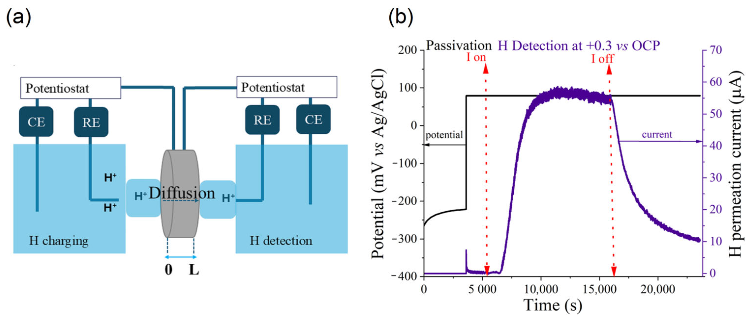
2.4. Electrochemical Permeation Test

The electrochemical permeation test is used to investigate the hydrogen diffusion in steel, and it was conducted using a hydrogen permeation cell (Devanathan and Stachurski cell) [15] consisting of two compartments (Figure 1a): the charging (or cathodic) cell where hydrogen is produced and the detection (or anodic) cell where hydrogen is detected. The surface of the sample exposed to the anodic and cathodic cell is 6.95 cm² (diameter 3 cm). Both cells are equipped with three electrodes: Ag/AgCl (KCl sat) as reference electrode (RE), platinum as counter electrode (CE), and the sample under analysis as working electrode (WE). The three electrodes in the anodic and cathodic cell were connected to a potentiostat, respectively, which was operated in floating mode (Figure 1a).

The charging cell was filled with 0.1 M HCl (CAS Nr. 7647-01-0 Honeywell, Offenbach, Germany) containing 0.2 g/L As₂O₃ (CAS Nr. 033-002-00-5, Carlo Erba Reagents S.r.l, Cornaredo, (MI), Italy). The detection cell was filled with 0.1 M NaOH (CAS Nr. 1310-73-2 Chem-lab, Zedelgem, Belgium). The measurements were conducted with the solutions open to the air.

The hydrogen permeation experiments followed precise timing (Figure 1b). First, the H-detection cell was filled with 0.1 M NaOH solution, and the open circuit potential (OCP) of the sample was recorded for 3600 s. Then, an anodic potential of +0.3 V vs. OCP was applied in the detection cell. The passivation current decreased with time, reaching values lower than 0.1 µA/cm². Then, the charging cell was filled with 0.1 M HCl and 0.2 g/L As₂O₃ solution, and the OCP of the steel was measured for 300 s; this was followed by a galvanostatic cathodic polarization applying a current equal to −6 mA. The area of the sample exposed to the solutions is 6.95 cm². After 3600 s at the OCP, a potential of +0.3 V vs. OCP was applied; a sudden increase in the current was recorded, and it was necessary to wait until 6000 s to reach a stable and low current value (about 1 μA) at the detection side before applying the H production current.

The hydrogen permeation curve consists of three phases [16]: build-up, in which hydrogen entry and diffusion occur with an associated increase in current (i) until reaching a plateau, called steady state (i_ss). A decay is then observed, in which hydrogen de-trapping occurs.

From the permeation curve, the diffusion coefficient (D_eff (m²/s)) can be calculated using two methods, the time lag method (Equation (1)) and the breakthrough time method (Equation (2)) [24]:

• t_lag method:

  $${\mathrm{D}}_{\mathrm{e}\mathrm{f}\mathrm{f}}={\displaystyle \frac{{\mathrm{L}}^2}{6{\mathrm{t}}_{\mathrm{l}\mathrm{a}\mathrm{g}}}},$$

  (1)
• Breakthrough method:

  $${\mathrm{D}}_{\mathrm{e}\mathrm{f}\mathrm{f}}={\displaystyle \frac{{\mathrm{L}}^2}{15.3{\mathrm{t}}_{\mathrm{b}}}},$$

  (2)

  where L is the thickness in meters of the sample, t_lag is the time (s) required to achieve 63% of steady state current density (i_ss), and t_b is the breakthrough time (s) that corresponds to the intersection of the tangent line at the inflection point and the x-axis in the permeation curve.

The subsurface concentration of diffusible hydrogen, C₀, can be determined by Equation (3) [25]:

$${\mathrm{C}}_0={\displaystyle \frac{{\mathrm{i}}_{\mathrm{s}\mathrm{s}}\mathrm{L}}{\mathrm{F}{\mathrm{D}}_{\mathrm{e}\mathrm{f}\mathrm{f}}}}{\displaystyle \frac{{\mathrm{M}}_{\mathrm{H}}}{{\mathsf{\rho }}_{\mathrm{F}\mathrm{e}}}}{10}^6,$$

(3)

where i_ss is the steady state permeation current density (A/m²), L is the thickness of the sample (m), D_eff is the effective diffusion coefficient (m²/s), F is the Faraday constant (96,485 C/mol), M_H is the molar mass of hydrogen (1 g/mol), and ρ_Fe is the iron density (7.87 × 10⁶ g/m³).

The data reported in this work are the mean values over at least three independent measurements. The standard deviations are given in parentheses in agreement with the guidelines published in [26].

3. Results

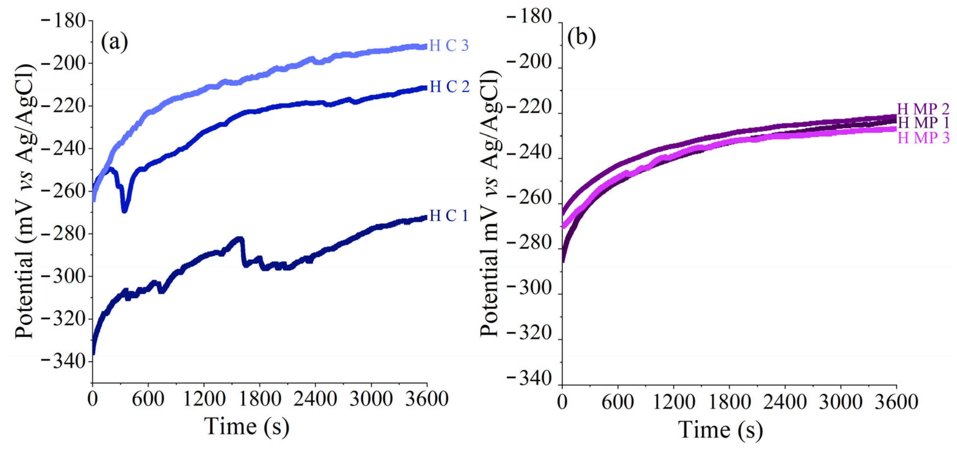
3.1. Conditioning of the Sample Surface Exposed to the Detection Side

The detection cell is filled with 0.1 M NaOH. The samples were conditioned by first exposing them to the NaOH solution and measuring for one hour the open circuit potential (OCP). The OCP versus exposure time curves for heated cleaned (H C X60) and mechanically polished (H MP X60) steel are shown in Figure 2. The open circuit potential increases asymptotically over time.

The potential immediately after immersion is at about −270 mV Ag/AgCl and reaches about −220 mV Ag/AgCl after one hour. The samples H MP X 60 steel are very reproducible (Figure 2b), and the H cleaned steel C X60 shows one outliner (Figure 2a).

Following the OCP measurement, the steels are passivated anodically at a potential +0.3 V vs. OCP. This procedure shall minimize the variation in surface conditions of the steel, prevent specimen oxidation, and increase the efficiency of the hydrogen atom oxidation reaction for more repeatable data [27]. The passivation current decreased following a power law and reached values below 0.5 µA, thus lower than 0.1 µA/cm² (

Table 2. Open circuit potential (mV vs. Ag/AgCl) measured after 1 h of exposure to the solution and current after 1 h of passivation; standard deviations calculated over three independent measurements are in parentheses.

	OCP (1 h, 0.1 M NaOH) (mV vs. Ag/AgCl)	Passivation Current (After 1 h) (µA)
H C X60 steel	−226 (42)	0.4 (0.3)
H MP X60 steel	−224 (3)	0.5 (0.2)

).

3.2. Conditioning of the Sample Surface Exposed to the Production Side

The production cell was filled with 0.1 M HCl solution containing 0.2 g/L As₂O₃; arsenic oxide inhibits the recombination reaction of hydrogen and promotes the formation of hydrogen atoms. The samples were exposed for 5 min to this solution, and also, in this case, the OCP was measured. Afterward, the cathodic hydrogen production with a current of −6 mA was started. The value measured on H C X60 steel in 0.1 M HCl (−435 (5) mV vs. Ag/AgCl) is slightly lower than the OCP value recorded on H MP X60 steel (−415 (10) mV vs. Ag/AgCl). The potential during cathodic polarization with a current of −6 mA was found at −996 (4) mV vs. Ag/AgCl for H C X60 steel and at −1067 (83) mV vs. Ag/AgCl for H MP X60 steel.

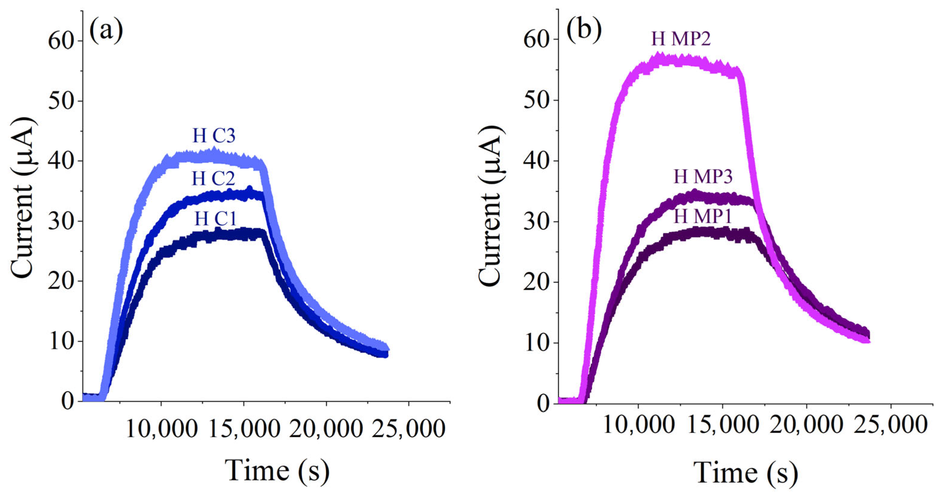
3.3. Hydrogen Permeation Results

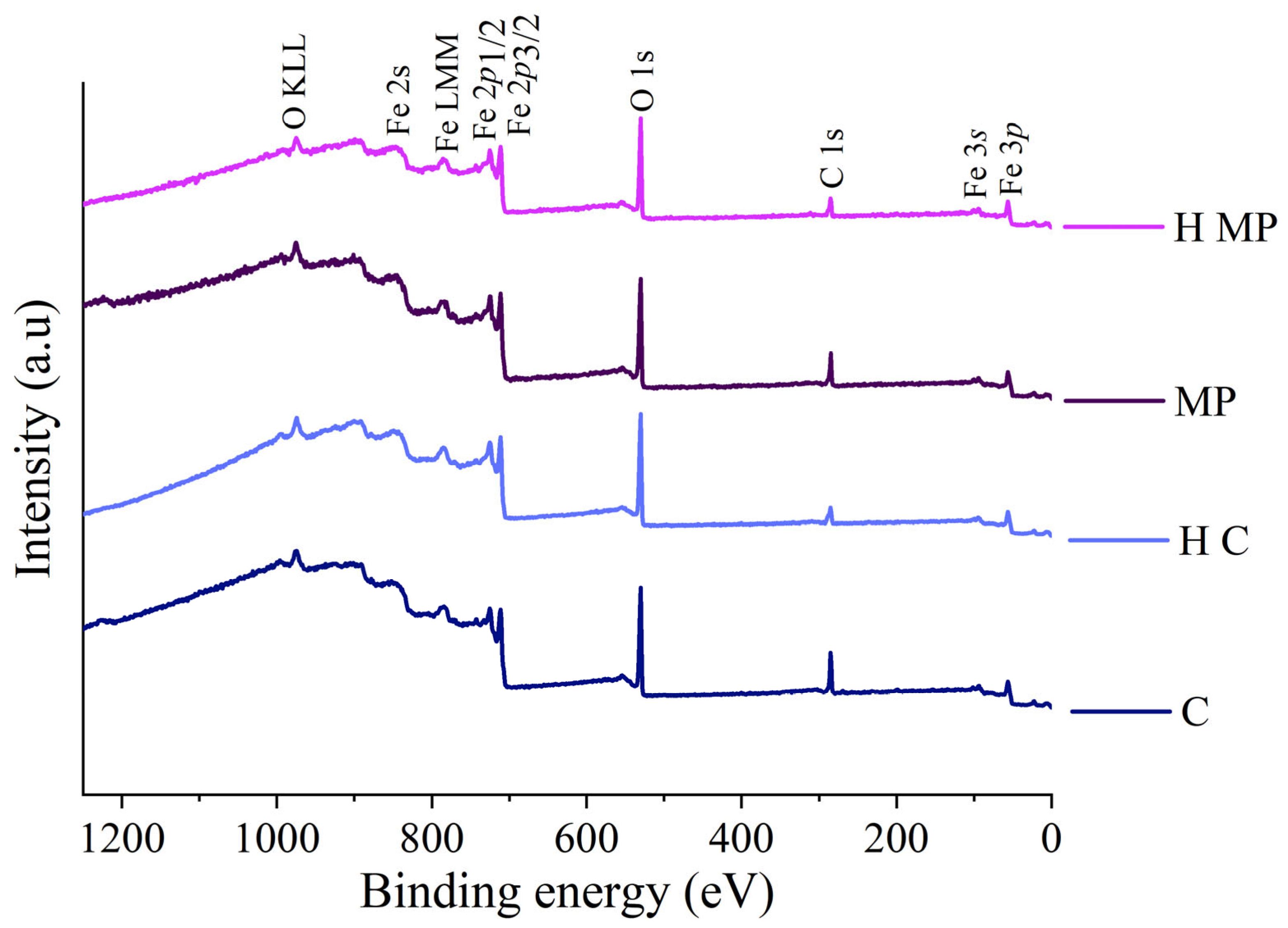
The anodic current at the detection cell was recorded continuously (Figure 3). After the start of hydrogen production, the current first remained very low, being almost 0 µA; afterward, it rapidly increased during the build-up phase and reached a nearly steady-state value.

After switching off the hydrogen production current, the anodic current in the detection cell decreased (decay phase).

The hydrogen permeation curves obtained on the cleaned H C X60 steel samples (Figure 3a) showed good reproducibility; the current due to hydrogen oxidation starts to increase, and the values of the steady state current, i_ss, are found to be 29.4 µA, 35.7 µA, and 41.8 µA for three repeated measurements. The hydrogen permeation curves of three mechanically polished MP X60 steel samples (Figure 3b) showed a similar behavior of the build-up and decay phases. The current due to hydrogen oxidation starts to increase; the i_ss values are found to be 29.0 µA, 57.9 µA, and 35.0 µA for the three samples.

The effective hydrogen diffusion coefficient was calculated for each permeation test using the time lag (t_lag) and the breakthrough (t_b) methods according to Equations (1) and (2); the results are reported in

Table 3. Effective diffusion coefficients (D_eff) and subsurface concentration C₀ values for H C X60 and H MP X60 steels. The results are reported as mean values over three independent measurements, and the standard deviations are given in parentheses.

	Deff-tlag Method (10−10 m2/s)	Deff-tb Method (10−10 m2/s)	C0 (ppm a)
H C X60 steel	2.4 (0.4)	2.8 (0.2)	0.66 (0.02)
H MP X60 steel	2.0 (0.4)	2.9 (0.5)	0.8 (0.1)

^a ppm: parts per million represent the mass fraction of hydrogen in iron, measured as milligrams of hydrogen per kilogram of iron.

. The values of the effective diffusion coefficient D_eff are found to be about 2 × 10⁻¹⁰ m²/s. No significant differences have been observed in the diffusion coefficient values for the cleaned and mechanically polished samples and between the two methods.

The subsurface concentration of hydrogen calculated using Equation (3) is shown in Table 3; the subsurface hydrogen concentration is slightly higher in the H MP X60 steel (0.8 (0.1) ppm) than in H C X60 steel (0.66 (0.02) ppm).

3.4. XPS Results

The surface of X60 steel samples was analyzed by XPS. This technique provides information on the composition of the surface, the chemical state of iron, the thickness of the oxide layer, and the hydrocarbon contamination layer following the different steps of the sample preparation, such as cleaning, mechanical polishing, and heat treatment for 15 h at 80 °C.

The survey spectra provide an initial overview (Figure 4). Fe signals are detected at the surface of cleaned and mechanically polished X60 samples both before and after heating at 80 °C for 15 h. In addition, C and O signals are observed. Their presence can be ascribed to surface contamination and oxidation of the outer layer of the steel due to the exposure of the samples’ surface to the ambient following the cleaning, heating procedures, and the sample transfer to the spectrometer.

Detailed information was obtained from the curve fitting of the high-resolution spectra (Figure 5). The curve fitting parameters of O 1s and Fe 2p signals are listed in Table S1 (Supporting Information). The Fe 2p_3/2 peak of the H C X60 steel and H MP X60 steel (Figure 5a,c) were curve-fitted according to the literature [28] and showed four components. The peak energy of metallic iron (Fe (0)) was found to be 706.8 (0.1) eV for both cleaned and MP X60 steel and 707.0 (0.1) eV for heated cleaned and heated MP X60 steel; Fe (II) oxide (FeO) was found at an energy value of 709.4 (0.1) eV with its satellite at 714.9 (0.1) eV; the peak energy of Fe (III) oxide (Fe₂O₃) was 710.6 (0.1) eV and for Fe (III) oxy-hydroxides (FeOOH) it was found to be 712.5 (0.1) eV [28].

The peak energies of each component are reported in

Table 4. Peak energy values (eV) of O 1s, Fe 2p_3/2 XP-signals of X60 steel reported as mean values over three independent measurements. The standard deviations are given in parentheses.

Elements	C X60 Steel Peak Energy (eV)	Heated C X60 Steel Peak Energy (eV)	MP X60 Steel Peak Energy (eV)	Heated C X60 Steel Peak Energy (eV)
O 1s–Oxide	530.1 (0.1)	530.2 (0.1)	530.1 (0.1)	530.2 (0.1)
O 1s–Hydroxide	531.4 (0.1)	531.4 (0.1)	531.4 (0.1)	531.5 (0.1)
O 1s–Water	532.2 (0.2)	532.2 (0.1)	532.2 (0.1)	532.3 (0.1)
O 1s–Organic	533.5(0.1)	533.4 (0.1)	533.5 (0.1)	533.5 (0.1)
contamination
Fe 2p3/2–Fe (0)	706.8 (0.1)	707.0 (0.1)	706.8 (0.1)	707.0 (0.1)
Fe 2p3/2–FeO	709.4 (0.1)	709.4 (0.2)	709.3 (0.1)	709.4 (0.1)
Fe 2p3/2–FeO sat	714.9 (0.1)	714.9 (0.2)	714.8 (0.1)	714.9 (0.1)
Fe 2p3/2–Fe2O3	710.6 (0.1)	710.7 (0.1)	710.6 (0.1)	710.6 (0.1)
Fe 2p3/2–Fe (III)-OOH	712.5 (0.1)	712.6 (0.1)	712.5 (0.1)	712.4 (0.1)

as mean values over three independent samples and analyzed in three areas each. The standard deviation in the text and in the table are given in parenthesis, as stated in the reference [26].

The O 1s signals showed four components; the peak energies of the components are at 530.1 (0.1) eV, 531.4 (0.1) eV, 532.2 (0.1) eV, and 533.5 (0.1) eV, and they are assigned to oxides, hydroxides, adsorbed water, and organic contamination, respectively [21] (Figure 5b,d and Table 4). Figure S2 (Supplementary Materials) shows the Fe 2p_3/2 and O 1s spectra after curve-fitting obtained on the solvent cleaned X60 steel and on the X60 after mechanical polishing but before heating.

The composition of the surface layer was calculated by taking into account the oxidized iron species, and the results are shown in

Table 5. Thickness of the contamination layer lc and the oxide layer t calculated applying the three-layer model for Cleaned, MP steel, and H C X60 and H MP X60 steels. Results are reported as mean values over three independent measurements, and the standard deviations are given in parentheses.

	C X60 Steel	Heated C X60 Steel	MP X60 Steel	Heated MP X60 Steel
lc (nm)	3.5 (0.8)	2.7 (0.3)	2.9 (0.5)	3.3 (0.2)
t (nm)	4.1 (0.5)	6.8 (0.9)	5.5 (0.7)	7.7 (0.5)
Atom % FeO	5 (2)	0.5 (0.7)	4 (3)	0.9 (0.9)
Atom % Fe2O3	60 (2)	64 (3)	62 (2)	64 (2)
Atom % FeOOH	35 (3)	36 (3)	34 (3)	35 (2)

. The three layers model allows calculating the thickness of the contamination layer (l_c) and of the oxide layer (t). The composition of the iron oxy-hydroxide film is similar in both samples.

4. Discussion

4.1. Surface Composition and Homogeneity

The peak energy values of Fe (II) oxide, Fe (III) oxide, and Fe (III)-OOH are in agreement with the literature [21,28,29], and they remained unchanged within the experimental uncertainty (0.1 eV) for all the samples regardless of the treatment (C X60, H C X60, MP X60 and H MP X60). The results of the peak binding energy values of nine analyzed areas on three independent samples are presented in Figure 6a. The component ascribed to metallic iron was found to be 0.2 eV higher after heating than before heating.

The thickness of the hydrocarbon contamination layer showed a small variation for the heated C X60 and for the heated MP X60 steels (Table 5) in comparison with the same samples before heating. The thickness of the oxide layers of the series of heated samples following both the cleaning with organic solvents and the mechanical polishing was higher than that of the same samples before heating. This suggests that the surface layer grows upon heating as expected. The standard deviation higher for the thickness values of the cleaned samples after heating might be interpreted as an indication of the growth of a non-homogeneous surface film. A more detailed analysis with a dot plot (Figure 6b) revealed that there are “outliers” that can be traced back to two points analyzed on two (of three) different samples. This indicates that the procedure of mechanical polishing leads to more reproducible surfaces, as indicated by the reproducibility of the open circuit potential versus time curves (Figure 2) for the mechanically polished surfaces (Figure 2b). Studies have shown that mechanically polished steel exhibits a better reproducibility of passive film after immersion in aggressive solutions [30].

Based on the peak energies of both iron and oxygen signals, we can state that the surface film is made of iron oxyhydroxides. The iron is mainly present as Fe (III) (Table 5). After heating, the atomic percentage of FeO strongly decreases; the Fe (II) component in the fitted Fe 2p_3/2 spectrum almost disappears, and this can explain the high relative uncertainty, which characterizes this contribution to the signal after heating (Table 5; from 5 (2) % to about 0.5 (0.7) % for C X60 steel and from 4 (3) % to about 0.8 (0.9) % in the case of the MP X60 steel). This decrease might be due to the fact that heating promotes oxidation into more stable oxides, such as Fe₂O₃. This might be substantiated by the trend that indicates an increase in the atomic percentage of Fe₂O₃. This observation is in agreement with the findings that heating can alter oxidation states and reduce reactive species on the surface [31].

4.2. Hydrogen Diffusion Coefficient of X60

The effective hydrogen diffusion coefficient D_eff values (Table 3) calculated with the t_lag and t_b methods are comparable, and no influence of the sample preparation method can be revealed. This indicates that the hydrogen diffusion coefficient is governed by the bulk material properties and it seems that it is not affected by nanometer thick surface layers. These two methods (t_lag and t_b), used frequently in the literature [32,33], are based on the assumption that the diffusion of hydrogen in the metal can be described by Fick’s laws (Equations (4) and (5)) [34] where j is the hydrogen flux, D_eff is the effective hydrogen diffusion coefficient, C the hydrogen concentration, x the distance from the surface, and t the time.

$$\mathrm{j}\left(\mathrm{x},\mathrm{t}\right)=-{\mathrm{D}}_{\mathrm{e}\mathrm{f}\mathrm{f}}{\displaystyle \frac{\partial \mathrm{C}(\mathrm{x},\mathrm{t})}{\partial \mathrm{x}}},$$

(4)

$${\displaystyle \frac{\partial \mathrm{C}}{\partial \mathrm{t}}}={\mathrm{D}}_{\mathrm{e}\mathrm{f}\mathrm{f}}{\displaystyle \frac{{\partial }^2\mathrm{C}}{\partial {\mathrm{x}}^2}},$$

(5)

The solution of Fick’s laws depends on the boundary conditions and the system geometry. For the Devanathan and Stachurski electrochemical double cell (see experimental), the conditions are (1) a membrane of finite thickness L; (2) C = C₀ at x = 0, meaning a constant hydrogen concentration C₀ at the production side; and (3) C = 0 at x = L, meaning that the hydrogen concentration at the detection side of the membrane is zero.

The effective diffusion coefficients calculated for the H C X60 steel (2.4 (0.4) 10⁻¹⁰ m²/s) and for the H MP X60 steel (2.0 (0.4) 10⁻¹⁰ m²/s) are in the same order of magnitude (Table 3) and in agreement with literature data (Figure 7) [35]. The fact that D_eff determined that the time lag method (63% of steady state current) and the breakthrough method (about 5% of the steady state current) are nearly identical (see Table 3) indicates that the experiments reached the steady state (Figure 3). The highest values of D_eff are reported for Armco iron (6.2 × 10⁻⁹ m²/s) [36] and pure annealed iron (4 × 10⁻⁹ m²/s) [37]. The comparison of the literature data obtained using different steels (Figure 8) shows that the hydrogen diffusion coefficient D_eff of X60 steel in this work is similar to the one of X65 steel (2.3 × 10⁻¹⁰ m²/s) [35] and 3.5 × 10⁻¹⁰ m²/s [38]. Previous studies reported hydrogen diffusion coefficient to be 6.2 × 10⁻¹¹ m²/s and 5.1 × 10⁻¹¹ m²/s for different grade high-strength pipeline steels such as X70 C and X80 C steels, respectively [32]. High carbon steel exhibited a D_eff value equal to 2.2 × 10⁻¹¹ m²/s) [36].

The influence of different tempering temperatures on the hydrogen diffusion on low-alloy high strength steel (LAHSS) [33] showed that the hydrogen diffusion coefficient D_eff increased with tempering temperature (Figure 7) [33].

4.3. Hydrogen Sub-Surface Concentration (C₀) of X60 Steel

The study of hydrogen subsurface concentration in steels is critical for understanding hydrogen embrittlement. Hydrogen accumulation near the surface can initiate micro-cracks, which can propagate under mechanical stress, leading to a failure [33].

The sub-surface hydrogen concentration C₀ at the production side of the sample was calculated from the hydrogen permeation curves using Equation (3).

The subsurface hydrogen concentration C₀ of heated C X60 and MP X60 steel is given in

Table 6. Hydrogen subsurface concentrations of different steel present in the literature compared with those obtained in this work.

	* C0 (ppm)	* C0 mol H/m3	Ref.
Heated C X60 steel	0.66 (0.02)	5.2 (1.4)	This work
Heated MP X60 steel	0.8 (0.1)	6.3 (0.8)	This work
LAHSS steel T640	0.21	1.65	[33]
LAHSS steel T600	0.87	6.85	[33]
LAHSS steel T560	1.52	11.96	[33]
High carbon steel	6.09	47.5	[36]
Weld X80 steel	2.21	17.43	[39]
HAZ X80 steel	2.12	16.71	[39]
Base X80 steel	1.54	12.12	[39]
Annealed iron	0.022	0.17	[37]
Armco Iron	0.085	0.662	[36]

* The values written in italics are converted values.

, together with the literature data from other steels of different compositions, microstructure, and heat treatment. In literature, two different units are used to report hydrogen concentration: mol H/m³ and ppm (Table 6). The conversion factor is the iron density of 7.87 g/cm³; for the sake of clarity, this discussion uses only ppm. The lowest values of C₀ are reported for annealed iron (0.022 ppm) [37] and annealed Armco iron (0.085 ppm) [36]. The hydrogen concentration C₀ in low alloyed high-strength steel (LAHSS) at different tempering temperatures (560 °C, 600 °C and 640 °C) was found to be 1.52 ± 0.01 ppm, 0.87 ± 0.08 ppm and 0.21 ± 0.01 ppm, respectively [33]. The influence of welding was tested on X80 steel; the hydrogen concentration C₀ for weld, heat affected zone (HAZ), and base X80 steel were found to be 2.21 ppm, 2.12 ppm, and 1.54 ppm, respectively [39].

4.4. Influence of Steel Microstructure and Composition

The steel studied in this work is API 5L X60 steel. API 5L is the standard specification for pipelines of the American Petroleum Institute. The pipelines are made of carbon steel pipes used for oil and gas transmission. The abbreviation “X60” defines the minimum yield strength (60′000 psi or 415 MPa). This (high) strength is achieved through the addition of alloying elements such as manganese, silicon, and chromium. The steels “X65”, “X70” and “X80” have a higher yield strength.

It is now interesting to evaluate the effective diffusion coefficient D_eff and the sub-surface hydrogen concentration C₀ of the different iron-based materials (Figure 8). At first glance, a log-log plot of D_eff vs. C₀ results in an approximately linear relationship, representing a power law. A high effective diffusion coefficient D_eff is related to a very low hydrogen concentration C₀ and vice versa: this appears to be valid for various materials independently from the method applied for the calculation of D_eff and C₀. It is noteworthy that a wide range of materials, from annealed and Armco iron [36,37] over the X60 steels studied in this work to X80 base material, welded, and heat affected zone (HAZ) [39], as well as LAHSS steel, tempered at temperatures between 560 and 640 °C [33], are in agreement with this power law.

5. Conclusions

This investigation provides a detailed evaluation of the surface composition and hydrogen permeability of X60 steel in terms of hydrogen diffusion coefficient and subsurface hydrogen concentration. The comparison with the literature data for various steels is also discussed. The following conclusions can be drawn

• XPS analysis revealed the presence of a film composed of Fe (II) oxide, Fe (III) oxide, and Fe (III) oxyhydroxide on the steel substrate on both organic-solvents cleaned and mechanically polished X60 steel samples. The composition and the film thickness formed upon heating at 80 °C for 15 h at the surface of mechanically polished samples are more reproducible than in the case of films present on the steels following the cleaning procedure with organic solvents. The reproducibility of the sample preparation ensures the reproducibility of the electrochemical results.
• The effective diffusion coefficients D_eff of both H C X60 and H MP X60 steels, calculated using t_lag and t_b methods, are in agreement with the literature data. D_eff depends on the bulk properties of the steel; indeed, D_eff of X60 steel seems to be unaffected by the presence of a nanometric thick film constituted of iron oxy-hydroxides. The lower D_eff value of X60 steel compared to pure iron might be explained by the presence of higher carbon content or other alloying elements changing the microstructure.
• The subsurface hydrogen concentration C₀ in X60 steel was found to be equal to 0.66 (0.02) ppm for C X60 steel and to 0.8 (0.1) ppm for MP X60 steel is lower than in high-carbon steels and other high-strength pipeline steels such as X80. This may be attributed to its specific microstructure, which includes bainite and possible martensite with globular carbides.

References

1. Heiniger, S.P.; Fan, Z.; Lustenberger, U.B.; Stark, W.J. Safe Seasonal Energy and Hydrogen Storage in a 1: 10 Single-Household-Sized Pilot Reactor Based on the Steam-Iron Process. Sustain. Energy Fuels 2024, 8, 125–132. [Google Scholar] [CrossRef]
2. Haller, M.Y.; Carbonell, D.; Dudita, M.; Zenhäusern, D.; Häberle, A. Seasonal Energy Storage in Aluminium for 100 Percent Solar Heat and Electricity Supply. Energy Convers. Manage X 2020, 5, 100017. [Google Scholar] [CrossRef]
3. Mahajan, D.; Tan, K.; Venkatesh, T.; Kileti, P.; Clayton, C.R. Hydrogen Blending in Gas Pipeline Networks—A Review. Energies 2022, 15, 3582. [Google Scholar] [CrossRef]
4. Ohaeri, E.; Eduok, U.; Szpunar, J. Hydrogen Related Degradation in Pipeline Steel: A Review. Int. J. Hydrogen Energy 2018, 43, 14584–14617. [Google Scholar] [CrossRef]
5. Negi, A.; Elkhodbia, M.; Barsoum, I.; AlFantazi, A. Coupled Analysis of Hydrogen Diffusion, Deformation, and Fracture: A Review. Int. J. Hydrogen Energy 2024, 82, 281–310. [Google Scholar] [CrossRef]
6. He, Y.; Su, Y.; Yu, H.; Chen, C. First-Principles Study of Hydrogen Trapping and Diffusion at Grain Boundaries in γ-Fe. Int. J. Hydrogen Energy 2021, 46, 7589–7600. [Google Scholar] [CrossRef]
7. Faucon, L.E.; Boot, T.; Riemslag, T.; Scott, S.P.; Liu, P.; Popovich, V. Hydrogen-Accelerated Fatigue of API X60 Pipeline Steel and Its Weld. Metals 2023, 13, 563. [Google Scholar] [CrossRef]
8. Contreras, A.; Hernández, S.L.; Galvan-Martinez, R.; Vega-Becerra, O. Tension Tests Behavior of API 5L X60 Pipeline Steel in a Simulated Soil Solution to Evaluate SCC Susceptibility. MRS Online Proc. Libr. 2012, 1481, 1–10. [Google Scholar] [CrossRef]
9. Walallawita, R.; Hinchliff, M.C.; Sediako, D.; Quinn, J.; Chou, V.; Walker, K.; Hill, M. Evaluating the Effect of Blended and Pure Hydrogen in X60 Pipeline Steel for Low-Pressure Transmission Using Hollow-Specimen Slow-Strain-Rate Tensile Testing. Metals 2024, 14, 1132. [Google Scholar] [CrossRef]
10. Mohtadi-Bonab, M.A.; Eskandari, M.; Rahman, K.M.M.; Ouellet, R.; Szpunar, J.A. An Extensive Study of Hydrogen-Induced Cracking Susceptibility in an API X60 Sour Service Pipeline Steel. Int. J. Hydrogen Energy 2016, 41, 4185–4197. [Google Scholar] [CrossRef]
11. Sun, B.; Zhao, H.; Dong, X.; Teng, C.; Zhang, A.; Kong, S.; Zhou, J.; Zhang, X.-C.; Tu, S.-T. Current Challenges in the Utilization of Hydrogen Energy-a Focused Review on the Issue of Hydrogen-Induced Damage and Embrittlement. Adv. Appl. Energy 2024, 14, 100168. [Google Scholar] [CrossRef]
12. Hoschke, J.; Chowdhury, M.F.W.; Venezuela, J.; Atrens, A. A Review of Hydrogen Embrittlement in Gas Transmission Pipeline Steels. Corros. Rev. 2023, 41, 277–317. [Google Scholar] [CrossRef]
13. Chen, Y.-S.; Huang, C.; Liu, P.-Y.; Yen, H.-W.; Niu, R.; Burr, P.; Moore, K.L.; Martínez-Pañeda, E.; Atrens, A.; Cairney, J.M. Hydrogen Trapping and Embrittlement in Metals—A Review. Int. J. Hydrogen Energy 2024, in press. [CrossRef]
14. Young, G. Hydrogen Embrittlement in Nuclear Power Systems. In Gaseous Hydrogen Embrittlement of Materials in Energy Technologies; Woodhead Publishing: Sawston, UK, 2011; ISBN 978-1-84569-673-3. [Google Scholar]
15. Devanathan, M.A.V.; Stachurski, Z.; Tompkins, F.C. The Adsorption and Diffusion of Electrolytic Hydrogen in Palladium. Proc. R. Soc. London. Ser. A Math. Phys. Sci. 1997, 270, 90–102. [Google Scholar] [CrossRef]
16. Zakroczymski, T. Adaptation of the Electrochemical Permeation Technique for Studying Entry, Transport and Trapping of Hydrogen in Metals. Electrochim. Acta 2006, 51, 2261–2266. [Google Scholar] [CrossRef]
17. API 5L X60 Pipe Specifications (PSL1 & PSL2)—Octal Steel. Available online: https://www.octalsteel.com/resources/api-5l-gr-x60-pipe/ (accessed on 18 March 2025).
18. SPECTRO xSORT XHH03 XRF Handheld Analyzer. Available online: https://www.spectro.com/products/xrf-handheld-analyzer/www.spectro.com/products/xrf-handheld-analyzer/xsort-xhh03 (accessed on 18 March 2025).
19. ISO 15472:2010; Surface Chemical Analysis—X-Ray Photoelectron Spectrometers—Calibration of Energy Scales. International Organization for Standardization: Geneva, Switzerland, 2010. Available online: https://www.iso.org/standard/55796.html (accessed on 30 January 2025).
20. Fairley, N.; Fernandez, V.; Richard-Plouet, M.; Guillot-Deudon, C.; Walton, J.; Smith, E.; Flahaut, D.; Greiner, M.; Biesinger, M.; Tougaard, S.; et al. Systematic and Collaborative Approach to Problem Solving Using X-Ray Photoelectron Spectroscopy. Appl. Surf. Sci. Adv. 2021, 5, 100112. [Google Scholar] [CrossRef]
21. Hannachi, R.; Biggio, D.; Elsener, B.; Fantauzzi, M.; Rossi, A. X-Ray Photoelectron Spectroscopy Investigation of X60 Steel. Surf. Sci. Spectra 2024, 31, 024014. [Google Scholar] [CrossRef]
22. Rossi, A.; Eisener, B. XPS Analysis of Passive Films on the Amorphous Alloy Fe70 Cr10 P13 C7: Effect of the Applied Potential. Surf. Interface Anal. 1992, 18, 499–504. [Google Scholar] [CrossRef]
23. Ypma, T.J. Historical Development of the Newton-Raphson Method. SIAM Rev. 1995, 37, 531–551. [Google Scholar] [CrossRef]
24. Koren, E.; Hagen, C.M.H.; Wang, D.; Lu, X.; Johnsen, R.; Yamabe, J. Experimental Comparison of Gaseous and Electrochemical Hydrogen Charging in X65 Pipeline Steel Using the Permeation Technique. Corros. Sci. 2023, 215, 111025. [Google Scholar] [CrossRef]
25. Van den Eeckhout, E.; De Baere, I.; Depover, T.; Verbeken, K. The Effect of a Constant Tensile Load on the Hydrogen Diffusivity in Dual Phase Steel by Electrochemical Permeation Experiments. Mater. Sci. Eng. A 2020, 773, 138872. [Google Scholar] [CrossRef]
26. Ellison, S.L.R.; Williams, A. Eurachem/CITAC Guide: Quantifying Uncertainty in Analytical Measurement, 3rd ed.; Eurachem/CITAC: Teddington, UK, 2012; ISBN 978-0-948926-30-3. [Google Scholar]
27. Casanova, T.; Crousier, J. The Influence of an Oxide Layer on Hydrogen Permeation through Steel. Corros. Sci. 1996, 38, 1535–1544. [Google Scholar] [CrossRef]
28. Biggio, D.; Elsener, B.; Usai, G.; Fantauzzi, M.; Rossi, A. Surface Chemistry of Passive Films on Ni-Free Stainless Steel: The Effect of Organic Components in Artificial Saliva. Langmuir 2024, 40, 6824–6833. [Google Scholar] [CrossRef] [PubMed]
29. Elsener, B.; Pisu, M.; Fantauzzi, M.; Addari, D.; Rossi, A. Electrochemical and XPS Surface Analytical Study on the Reactivity of Ni-Free Stainless Steel in Artificial Saliva. Mater. Corros. 2016, 67, 591–599. [Google Scholar] [CrossRef]
30. Rossi, A.; Elsener, B.; Hähner, G.; Textor, M.; Spencer, N.D. XPS, AES and ToF-SIMS Investigation of Surface Films and the Role of Inclusions on Pitting Corrosion in Austenitic Stainless Steels. Surf. Interface Anal. 2000, 29, 460–467. [Google Scholar] [CrossRef]
31. Rossi, A.; Elsener, B.; Spencer, N.D. XPS Surface Analysis: Imaging and Spectroscopy of Metal and Polymer Surfaces; Spectroscopy Europe/World: West Sussex, UK, 2004; Volume 16. [Google Scholar]
32. Samanta, S.; Kumari, P.; Mondal, K.; Dutta, M.; Singh, S.B. An Alternative and Comprehensive Approach to Estimate Trapped Hydrogen in Steels Using Electrochemical Permeation Tests. Int. J. Hydrogen Energy 2020, 45, 26666–26687. [Google Scholar] [CrossRef]
33. Cheng, X.Y.; Zhang, H.X. A New Perspective on Hydrogen Diffusion and Hydrogen Embrittlement in Low-Alloy High Strength Steel. Corros. Sci. 2020, 174, 108800. [Google Scholar] [CrossRef]
34. Frappart, S.; Feaugas, X.; Creus, J.; Thebault, F.; Delattre, L.; Marchebois, H. Study of the Hydrogen Diffusion and Segregation into Fe–C–Mo Martensitic HSLA Steel Using Electrochemical Permeation Test. J. Phys. Chem. Solids 2010, 71, 1467–1479. [Google Scholar] [CrossRef]
35. Fallahmohammadi, E.; Bolzoni, F.; Lazzari, L. Measurement of Lattice and Apparent Diffusion Coefficient of Hydrogen in X65 and F22 Pipeline Steels. Int. J. Hydrogen Energy 2013, 38, 2531–2543. [Google Scholar] [CrossRef]
36. Hadam, U.; Zakroczymski, T. Absorption of Hydrogen in Tensile Strained Iron and High-Carbon Steel Studied by Electrochemical Permeation and Desorption Techniques. Int. J. Hydrogen Energy 2009, 34, 2449–2459. [Google Scholar] [CrossRef]
37. Drexler, A.; Siegl, W.; Ecker, W.; Tkadletz, M.; Klösch, G.; Schnideritsch, H.; Mori, G.; Svoboda, J.; Fischer, F.D. Cycled Hydrogen Permeation through Armco Iron—A Joint Experimental and Modeling Approach. Corros. Sci. 2020, 176, 109017. [Google Scholar] [CrossRef]
38. Yao, C.; Ming, H.; Chen, J.; Wang, J.; Han, E.-H. Effect of Cold Deformation on the Hydrogen Permeation Behavior of X65 Pipeline Steel. Coatings 2023, 13, 280. [Google Scholar] [CrossRef]
39. Xue, H.B.; Cheng, Y.F. Hydrogen Permeation and Electrochemical Corrosion Behavior of the X80 Pipeline Steel Weld. J. Mater. Eng Perform 2013, 22, 170–175. [Google Scholar] [CrossRef]
Figure 1. (a) Scheme of the electrochemical hydrogen permeation test set-up; (b) example of hydrogen permeation curve and timing.
Coatings 15 00442 g001
Figure 2. Open circuit potential (mV vs. Ag/AgCl) vs. time curves for hydrogen permeation curves (hydrogen detection current vs. time) for (a) three cleaned X60 steel samples after heating (H C1, H C2, H C3), (b) three mechanically polished X60 steel after heating (H MP1, H MP2, H MP3). H means heated; C means cleaned; MP means mechanically polished.
Coatings 15 00442 g002
Figure 3. Hydrogen permeation curves (hydrogen detection current vs. time) for (a) three cleaned X60 steel samples (H C1, H C2, H C3), (b) three mechanically polished X60 steel (H MP1, H MP2, H MP3). H means heated; C means cleaned; MP means mechanically polished. The start of hydrogen production is at t = 0 (refer to Figure 1b at 6000 s).
Coatings 15 00442 g003
Figure 4. Survey spectra for cleaned (C), heated cleaned (H C), mechanically polished (MP), and heated MP (H MP) X60 steel.
Coatings 15 00442 g004
Figure 5. Fe 2p3/2 and O 1s peaks recorded on H C X60 steel (a,b) and H MP X60 steel (c,d).
Coatings 15 00442 g005
Figure 6. (a) Dot plot of the peak energies of Fe 2p3/2 components for cleaned (C), Heated C (H C), and MP, Heated MP (H MP) steels. (b) Dot plot of oxide layer thickness (t) calculated using the three-layer model for MP, C, H C and H MP X60 steels.
Coatings 15 00442 g006
Figure 7. Comparison of literature data on the effective diffusion coefficient of iron, steel, and high-strength steel with the data of this work [32,33,35,36,37,38,39].
Coatings 15 00442 g007
Figure 8. Comparison of the effective diffusion coefficient Deff and the subsurface hydrogen concentration C0 for different iron and steel grades from literature, ◁ [33], ◊ [36], □ [37], ◯ [39].
Coatings 15 00442 g008