Temporal and Spatial Variation Study on Corrosion of High-Strength Steel Wires in the Suspender of CFST Arch Bridge

Abstract

The corrosion and degradation behavior of high-strength steel wires during service directly affect the safety and usability of suspenders in steel pipe concrete arch bridges. In this study, three different types of specimens were fabricated using steel wires extracted from the suspenders of an 11-year-old in-service arch bridge and subjected to accelerated corrosion tests with acetic acid. Considering the differential diffusion processes of corrosion factors caused by varying degrees of damage to the suspender sheath, the spatial corrosion variability of steel wires at different positions within the suspender cross-section was investigated. Experimental results indicated a two-stage characteristic in the corrosion process of individual galvanized steel wire samples. In the first corrosion stage, the microstructure on the corroded steel wire surface evolved from a dense crystalline structure to a porous one. In the second corrosion stage, corrosion products accumulate on the steel wire substrate, subsequently further aggregating into sheet-like structures. The maximum pitting factor of individual steel wire samples from a specific area could be described by a Type I extreme value distribution. In the time-dependent model that was established, the location parameter and scale parameter exhibited an exponential decrease during the first corrosion stage and a linear decrease during the second corrosion stage. In the absence of sheath protection, the coefficient of variation in corrosion among adjacent steel wires in the suspender followed a normal distribution. The spatial corrosion variability of the wires inside the suspender is significantly influenced by the shape of the suspender sheath damage. As the corrosion time increased, the overall discrepancy in corrosion levels among different layers of wires diminished.

1. Introduction

In the management of the complete service life cycle of steel tube concrete arch bridges, the performance of suspenders and the steel wires inside them is a crucial consideration. Previous field surveys have indicated that under the influence of complex stresses, there is a probability of damage to the outer layer sheath of the suspenders, leading to the infiltration of water molecules and causing electrochemical corrosion inside the suspenders [1]. During the service life of a bridge, highly humid areas may develop within the suspender, leading to corrosion of the steel wires. Consequently, this deterioration in the overall load-bearing performance of the suspender significantly shortens the service life of the bridge compared to its designed lifespan [2,3,4,5,6]. Establishing a model for the apparent description of corrosion in steel wires and suspenders and studying the spatiotemporal variability of their corrosion states is essential for estimating the residual bearing capacity, assessing the service life, formulating maintenance strategies, and making decisions on suspender replacement for large-span steel tube concrete arch bridges.

The assessment of corrosion levels in the suspender requires characterization based on the degree of corrosion of the steel wires and the distribution of rust damage within it [7]. Regarding environmental factors and stress effects, Suzumura and Nakamura studied the influence of sodium salt and relative humidity on high-strength steel wires [8]. Wu et al. investigated the phenomenon of premature failure caused by stress corrosion cracking in corroded steel wires under specific environmental conditions [9]. Chen et al. conducted corrosion experiments on individual steel wires using an electric current-accelerated corrosion method. They observed and analyzed the surface condition of corroded steel wires and further investigated their mechanical properties [10]. Li et al., concerning the corrosion behavior and corrosion rate of steel wires under the attack of corrosion factors, modeled the uniform corrosion process and pitting corrosion process through corrosion tests, providing examples based on practical engineering [11,12]. Karanci monitored the internal conditions of suspenders to obtain environmental parameters and established an annual corrosion rate model for the main cables of suspension bridges [13]. Xue and Shen, considering corrosion randomness, numerically simulated the constitutive model of wires under different corrosion levels [14]. In the study of steel wire pitting, Xu Li built a three-dimensional model of corroded steel wires and performed statistical analysis of corrosion pits using image processing techniques [15]. Fang et al. investigated the development of corrosion pits in stressed steel wires [16]. Rou Li investigated the corrosion rate characteristics of steel wires under the coupled effects of multiple factors by adjusting the pH value of the corrosive solution and sodium salt concentration, combined with stress effects [17,18]. Wang simplified the stochastic corrosion pits caused by electrochemical corrosion, prepared simulated damage pits using mechanical cutting, and studied the mechanical properties of damaged steel wires [19]. The preceding discussion elucidated the corrosion process and distribution of corrosion damage in steel wires, followed by a discussion and investigation of the close relationship between the surface characteristics of steel wires and their performance.

Corrosion pits can alter the surface morphology of steel wires, causing stress concentration and significantly reducing the fatigue life of components [20,21,22]. Liu integrated fatigue testing machines and electrochemical corrosion devices, studying the mechanical properties of steel wires under static and fatigue conditions simultaneously [23]. Zheng et al. utilized steel wires extracted from the suspenders of an arch bridge that had been in service for 13 years. These wires were subjected to different corrosion environments, resulting in four types of corroded wires. The relationship between the surface corrosion state and the mechanical properties of the wires was investigated. Additionally, residual life predictions were proposed based on environmental conditions and initial pitting depth [24]. Jiang et al. conducted profile measurements and fatigue tests on steel wires with six different corrosion levels and described the corrosion pits on the surface of corroded steel wires using mathematical methods. They established an empirical formula for calculating fatigue life, considering the corrosion effect [25]. Regarding the impact of corrosion on fatigue performance, Lan, Wang, and others proposed methods for predicting the remaining fatigue life of steel wires [26,27,28]. Deng, based on this, studied the two-stage characteristics of corroded steel wire life [29]. In normal service states, corrosion factors and fatigue loads act simultaneously on the high-strength steel wires composing the suspenders. To assess the service performance of steel wires more comprehensively, corrosion fatigue performance has also received widespread attention, including damage evolution simulation, fatigue crack initiation, and assessment of residual usage performance [30,31,32]. Wang, using a combined experimental and simulation approach, studied the damage evolution process of pre-existing notches in steel wires under the coupling action of fatigue loads and corrosion factors and predicted the service life of steel wires [33]. Miao, by preparing pre-existing notches on steel wires, revealed the influence of pits and stress amplitude on the fatigue life of steel wires under simultaneous mechanical and electrochemical corrosion [34]. Considering notch size, spacing, and angle between adjacent notches based on pre-made notches, Chen used finite element software to evaluate the life of steel wires [35]. Many bridges have entered the maintenance phase, and the detection and inspection of the internal corrosion of suspenders have received increasing attention in recent years [36]. The development and improvement of techniques such as self-leakage magnetism and non-contact mapping also provide effective means for addressing such issues [37,38,39].

In summary, despite the extensive focus of many studies on the corrosion process of individual steel wires, there remains a dearth of specific characterization regarding the overall corrosion process and description of corrosion states in suspenders. This study focuses on conducting acetic acid salt spray accelerated corrosion tests on specimens of various types fabricated from steel wires extracted from within the suspension rods of arch bridges. Subsequently, electron microscopy is employed to obtain detailed features of the microstructure of corroded surfaces. Furthermore, a targeted description of the spatiotemporal variability of the corrosion state of steel wires within simulated damaged suspension rod specimens is provided. The changes in the microstructure of corroded steel wire surfaces were discussed, and models were established to depict the variation in corrosion depth, surface roughness of steel wires, and corrosion heterogeneity over time. The statistical models established based on experimental results can provide a reference for assessing the temporal and spatial variability of steel wires during the overall corrosion process of suspenders.

2. Accelerated Corrosion Salt Spray Test

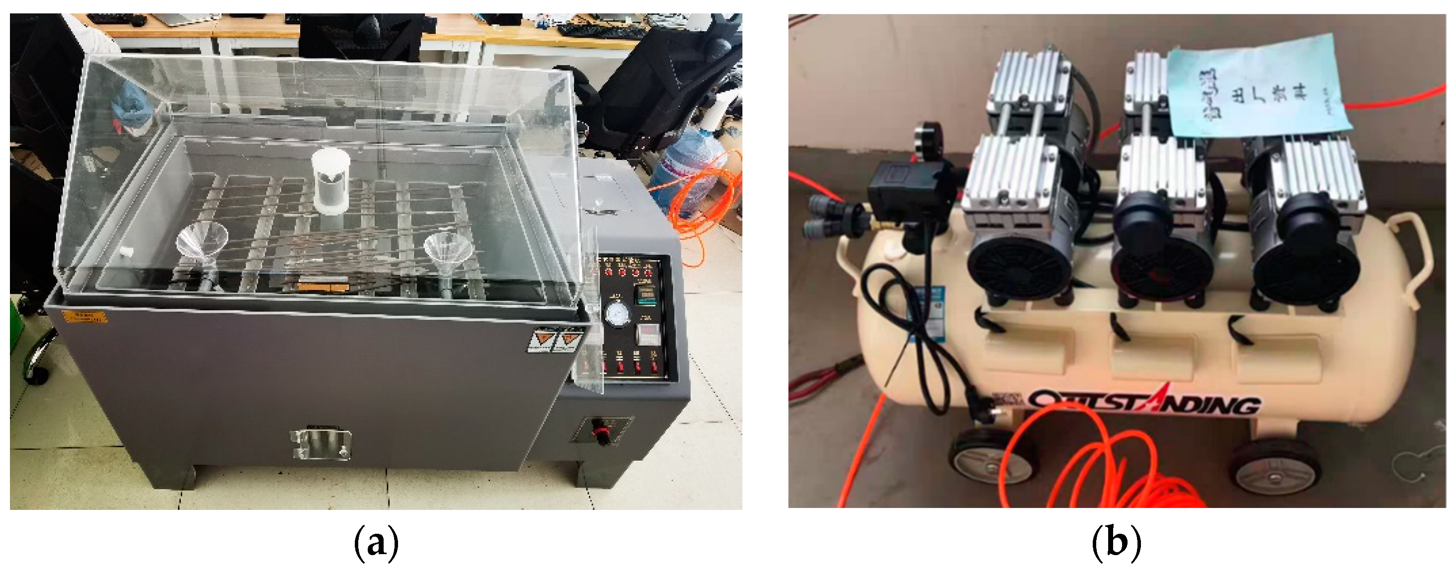
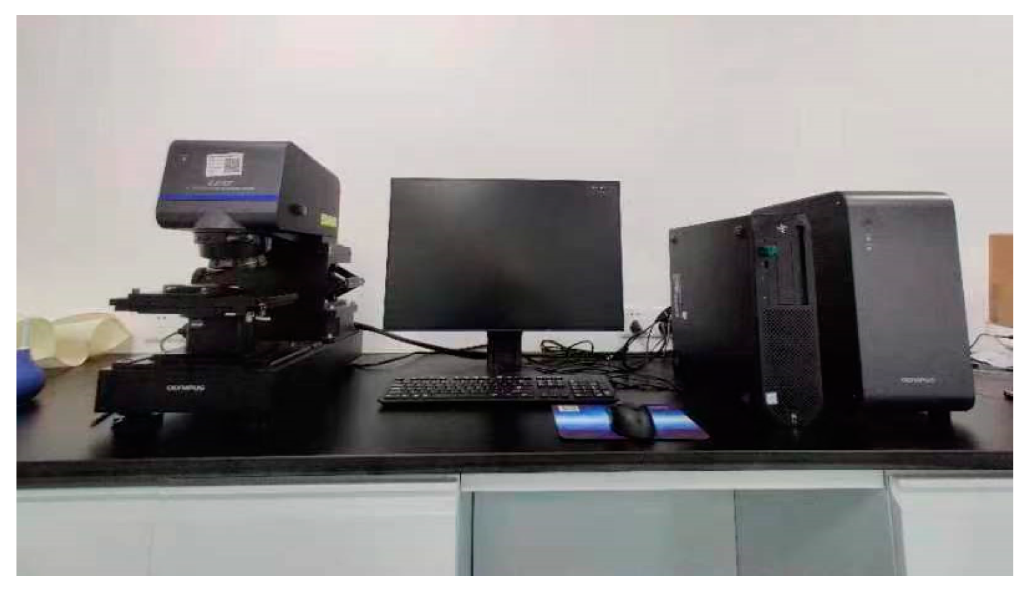
2.1. Experimental Equipment

The corrosion test was conducted using the salt spray test machine shown in Figure 1. The external dimensions of the chamber are 134 mm × 820 mm × 1080 mm, and the internal dimensions are 900 mm × 500 mm × 600 mm. The salt spray test machine utilizes Bernoulli’s principle to draw the corrosive liquid, pressurize and atomize it through an air compressor, and evenly spray the atomized corrosion solution inside the test chamber using nozzles. Simultaneously, the temperature sensing system maintains the temperature within the specified range to ensure a stable corrosive environment inside the chamber, with the corrosion environment temperature set at 35 °C for acetic acid salt spray corrosion tests.

The accelerated corrosion test employed acetic acid salt spray (AASS) following the standards outlined in ISO 9227:1990 [40]. A salt solution was prepared using solid NaCl crystals with a purity of 99.5%, and the concentration of sodium chloride in the salt solution, prepared with pure water, was adjusted to 50 g/L ± 5 g/L. An appropriate amount of glacial acetic acid was then added, and the pH of the corrosion solution was adjusted to 3.0. The corrosion solution was atomized using the salt spray test machine. The detailed conditions during the operation of the salt spray test machine are shown in

Table 1. Accelerated corrosion test details.

Salt Spray Type	Spray Method	Spray Rate	pH	Rust Solution Components	Test Temperature
Acetic acid and salt spray	Continuous spraying is carried out with non-crystallizing nozzle and tower spray device	(1~2) mL/h in the range of 8000 mm2	3.0	Sodium chloride, glacial acetic acid	35 °C

.

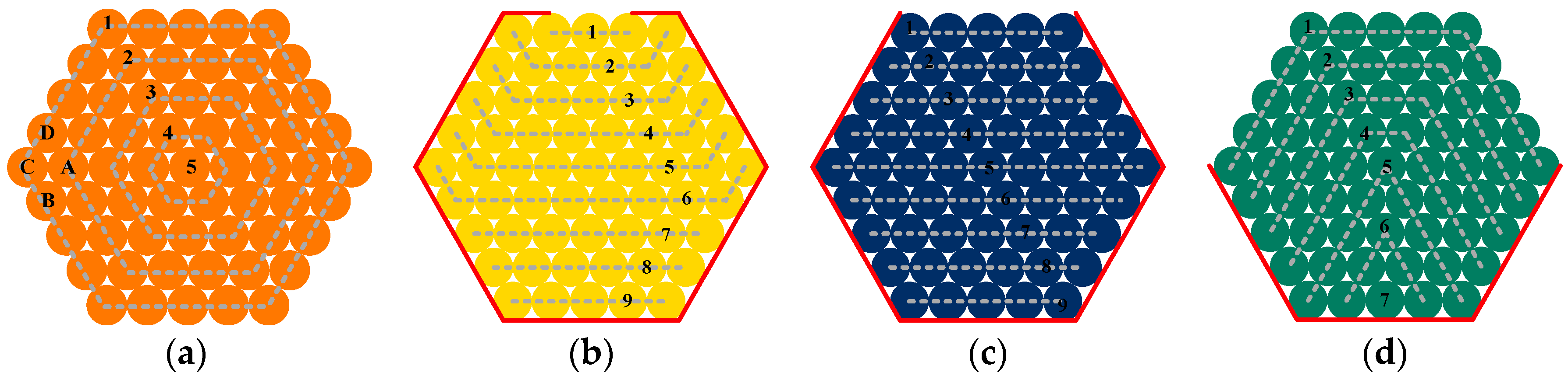
2.2. Spatial Variability of Suspender Steel Wire

The bridge utilizes the OVMLZM-I parallel steel wire cold anchoring system. The suspender consists of 61 parallel steel wires to achieve sufficient load-bearing capacity. To achieve the predetermined experimental objectives, three different specimens were fabricated using suspension rod wires disassembled from the original bridge. The nominal diameter of the steel wires composing the suspender is 7 mm, with an ultimate tensile strength of 1670 MPa. The zinc coating mass on the surface of the steel wires exceeds 338 g/m². The chemical composition of the specimen is provided in

Table 2. Chemical composition of steel wire, excluding iron elements.

Compositions	C	Si	Mn	S	Cu	Cr
wt.%	0.85–0.90	0.12–0.32	0.60–0.90	≤0.0025	≤0.10	0.10–0.25

. The overview of the specimen fabrication process is as follows:

(1)

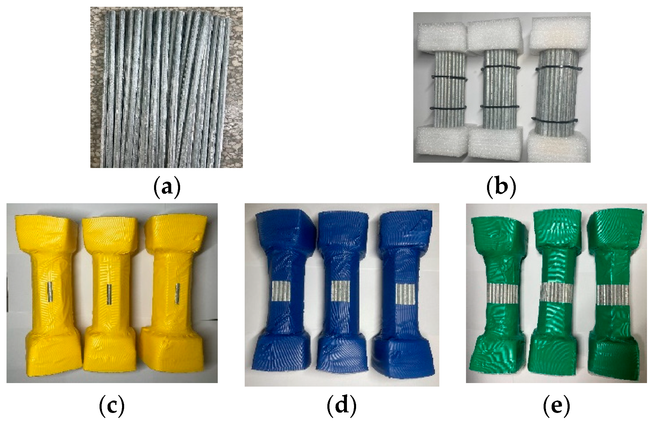
Type I Specimens (Single wire specimen): The wires disassembled from the suspenders were cut into 200 mm steel bars. The specimens were cleaned with ethanol and labeled, as shown in Figure 2a. These specimens were employed to investigate the evolving corrosion states of individual steel wires during accelerated corrosion testing and the corresponding microstructural changes on the corroded steel wire surfaces.

(2)

Type II Specimens (Protection failure specimen): Comprising 61 wires, each 200 mm in length, these specimens were bundled according to the original arrangement of wires within the suspenders. Before bundling, the steel wire needs to be cleaned, weighed, and properly labeled. The ends of the wire bundle were secured using custom-made polytetrafluoroethylene molds, as depicted in Figure 2b. The specimens with complete failure of simulated suspender corrosion protection measures can be utilized to investigate the differences in the corrosion development process of the steel wires.

(3)

Type III Specimens (Sheath-damaged bundle specimens): Based on the Type II specimens, to simulate the protective sheath, the bundled wires were covered with waterproof material and further reinforced by wrapping with waterproof tape. This treatment ensures waterproofing and facilitates easy cutting to simulate various damaged forms on the protective material. Based on the results of field investigations on in-service bridges, three simulated damage forms are considered: (a) Strip-like damage, as shown in Figure 2c. (b) Rectangular sheath damage, as shown in Figure 2d. (c) Semi-circular damage, as shown in Figure 2e. Considering the impact of the shape of suspender sheath damage on the diffusion of corrosion factors, utilizing such specimens enables the exploration of spatial corrosion differences among suspender steel wires under different diffusion modes.

The three types of steel wire specimens were subjected to accelerated corrosion testing in a salt spray test chamber.

Table 3. Corrosion time of the steel wire specimen.

Type of Specimen	Accelerated Corrosion Time (Day)	Number of Test Specimens	Note
Type I	3	5	Horizontally placed.
	6	5
	9	5
	10	2
	12	5
	15	5
	18	5
	20	2
	21	5
	24	5
	27	5
	30	5
	31	2
	33	5
Type II	90	3	Horizontally placed with periodic rotation to ensure uniform corrosion across the specimen.
Type III	50	3	Vertically placed at 90 degrees.
	70	3
	90	3

provides the corrosion duration for each specimen. For Type I specimens, five specimens were prepared at each of the following corrosion periods: 3, 6, 9, 12, 15, 18, 21, 24, 27, 30, and 33 days. In order to comprehensively analyze the evolutionary trajectory of the steel wire corrosion process, meticulous documentation of the 11 distinct corrosion stages is imperative. Each corrosion stage necessitates the utilization of five specimens, aimed at elucidating the nuanced variations in wire corrosion behavior throughout the entirety of the corrosion process. Additionally, three sets of single steel wire specimens, each consisting of two specimens, were prepared for field emission scanning electron microscope observation of the microscopic surface morphology of corroded steel wires, corresponding to corrosion durations of 10, 20, and 31 days. These two sets of specimens were sufficient for preparing samples for scanning electron microscopy.

Due to the limited space within the salt spray chamber and the diverse range of specimens, it is necessary to control the quantity of various specimens. A rational allocation of specimens can prevent mutual interference among specimens from different hierarchies and ensure minimal disruption to experimental results. Simultaneously, specimens can be batched into the chamber, with a specific operational arrangement involving placing Type I specimens first, extracting them once the target corrosion time is completed, and subsequently introducing the next batch of specimens to utilize the chamber space effectively.

2.3. Derusting Process

To facilitate subsequent observation and analysis of the steel wire surfaces, it is necessary to conduct rust removal treatments on the steel wires. A 10% diluted hydrochloric acid reagent with a corrosion inhibitor was used to pick up the corroded high-strength steel wire. The corroded samples were placed in a glass container, diluted with hydrochloric acid, soaked for 5–6 min, and then cleaned. The acid-washed high-strength steel wire was placed in a Ca(OH)₂ solution to neutralize the residual hydrochloric acid on the surface, and then placed in clean water (not higher than 40 °C) to wash off the residual Ca(OH)₂ on the high-strength steel wire [41]. Finally, the steel wire was dried, as shown in Figure 3. The specimen was cut to a length of 50 mm for electron microscopy.

3. Statistical Analysis of Apparent Characteristics of Steel Wires

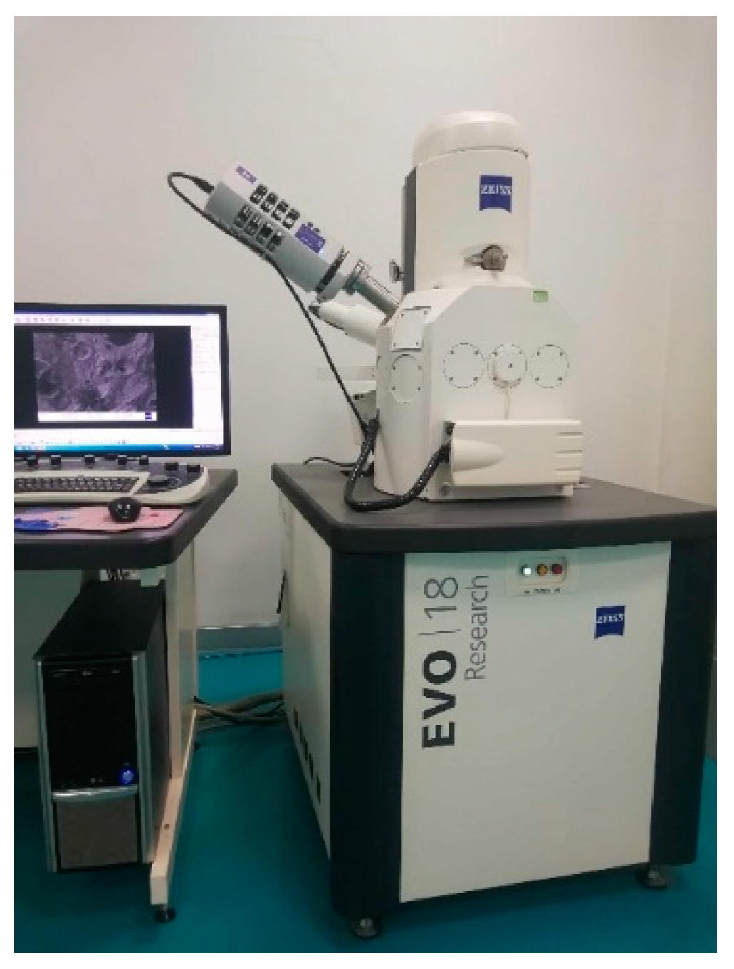
3.1. Microscopic Morphology of Corroded Steel Wires

Before conducting microscopic observations on the corroded steel wire samples, the macroscopic corrosion morphology changes of the Type I specimen were first introduced based on the salt spray test results, as shown in Figure 4. From the figure, it can be observed that in the initial stage of the corrosion experiment, white flocculent oxide of the galvanized layer gradually accumulated on the surface of the steel wire. When the corrosion time reached 15 days, the oxide of the galvanized layer peeled off, and the steel wire substrate was corroded. The color of the corrosion products gradually transitioned from white to yellow, and finally, starting after 24 days, reddish-brown oxides gradually covered the surface of the steel wire.

Field emission scanning electron microscopy (SEM) was employed for the examination of the surface morphology of corroded steel wires, as depicted in Figure 5. In the early stages of corrosion, minute cracks have been observed to initiate on the surface of the steel wire, as depicted in Figure 6. The volumetric expansion of corrosion products has led to the appearance of surface cracks on the steel wire. With the increasing exposure time of the steel wire in the corrosive environment, microscopic changes have gradually occurred on the corroded surface. Observations under an electron microscope at 5000× magnification revealed four stages of surface morphology changes in the steel wire, as illustrated in Figure 7. Initially, the galvanized layer appears intact, uniformly covering the steel wire substrate, as shown in Figure 7a. During the initial stages of corrosion, granular corrosion products from the galvanized layer adhere to the corroded area, gradually exposing the steel wire substrate, as shown in Figure 7b. As the corrosion progresses, uniformly small granular products accumulate, becoming more porous in morphology. At this stage, the corroding agents have fully accessed the steel wire substrate, resulting in the formation of iron oxide, which presents a cotton-like appearance, as depicted in Figure 7c. Upon prolonged exposure to the corrosive environment, abundant corrosion products from the steel wire substrate accumulate, exhibiting characteristics of layered stacking and a more porous physical state compared to previous products, as shown in Figure 7d.

It is noteworthy that, as the stacked corrosion products naturally peel off, corrosion pits are directly exposed on the surface of the steel wire substrate. Simultaneously, some scattered cracks appeared near the corrosion pits. As shown in Figure 8, it can be observed that corrosion pits lead to cross-sectional loss of the steel wire, coupled with stress concentration caused by the additional presence of cracks, which may significantly compromise the load-bearing capacity of the steel wire and reduce the performance of its products.

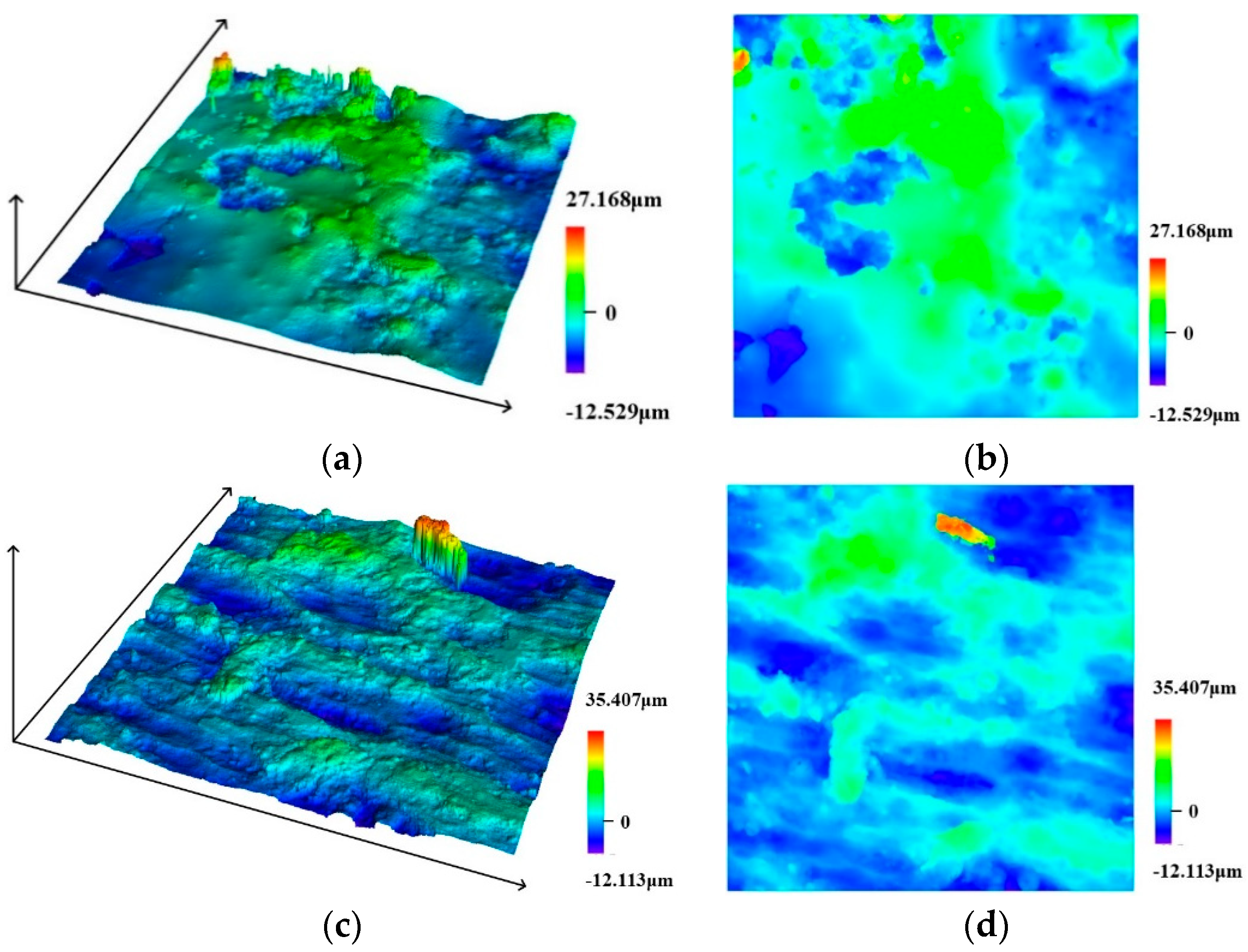
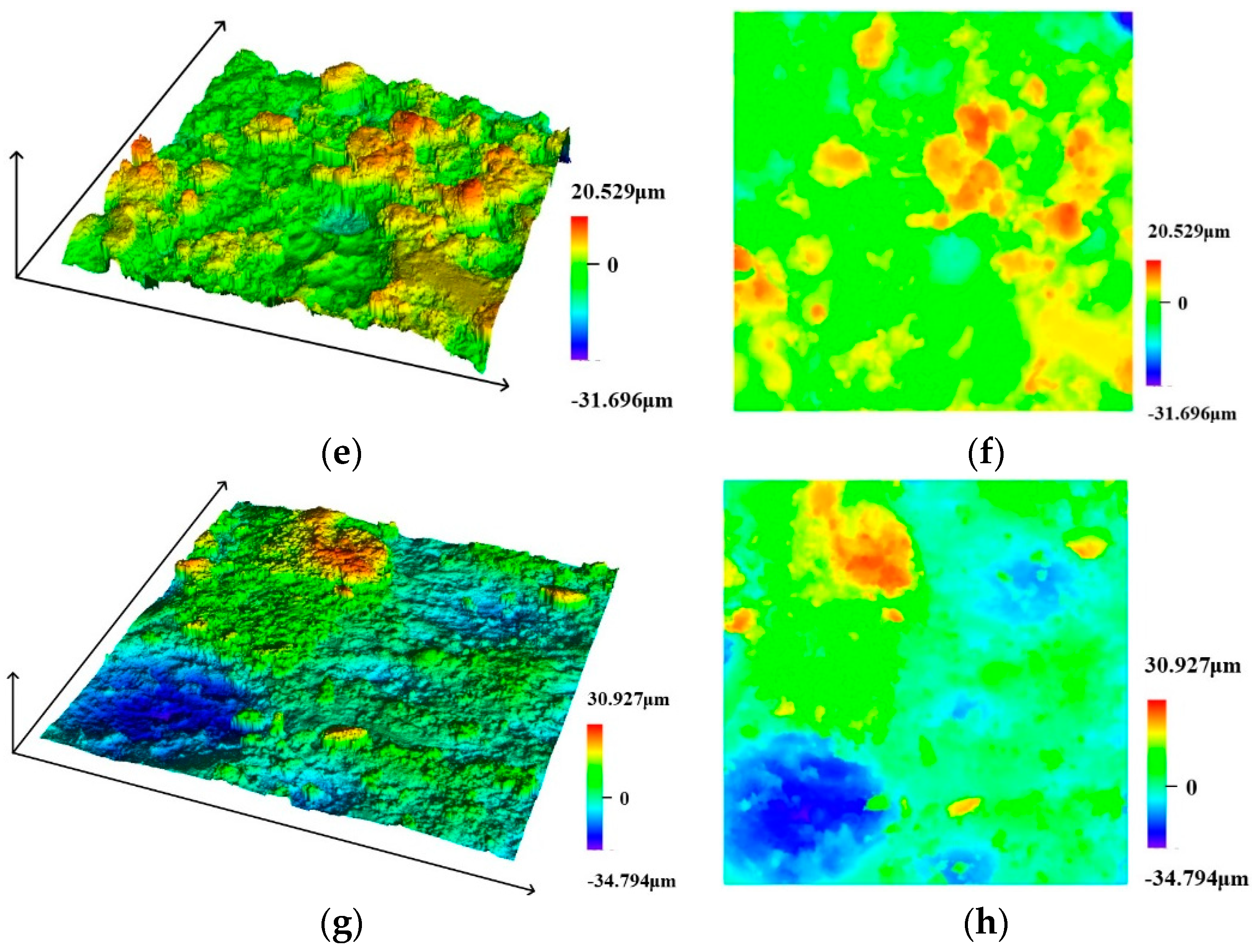
3.2. Surface Profile Measurement

The surface of corroded steel wires is uneven, and using two-dimensional contour plots can provide a reasonable and intuitive depiction of the elevation of the object’s surface. Roughness, denoted as RA, can be defined as the vertical deviation between the contour lines within the sampling area and the average contour line value of that area. Its mathematical expression is [42]:

$$R_a=\frac{1}{l}{\displaystyle {\int }_0^l\left|y(x)-y_m\right|dx\approx \frac{1}{k}{\displaystyle \sum _{i=1}^k\left|y_i-y_m\right|}}$$

(1)

where x is the coordinate of the contour length, y (x) is the contour height coordinate, y_m is the average contour height, y_i is the contour height of the i-th measurement point, and k is the total number of measurement points.

Where l denotes the total length of the sampling area; x denotes the length coordinate of the contour line, indicating its position; y (x) represents the height coordinate of the contour line, indicating its elevation value; y_m represents the average value of contour lines within the measurement area; y_i represents the value of the i-th measurement point’s contour line, and k represents the total number of measurement points.

The steel wire specimens were scanned using a confocal laser scanning microscope to examine the surface (accuracy 0.12 μm). The equipment used in this study is shown in Figure 9. Typical surface scan results for the steel wire are shown in Figure 10. The surface conditions of the steel wire can be more intuitively visualized with 3D scanning and contour maps. The initial state of the steel wire surface appears relatively smooth, with a dense zinc coating covering the surface, as depicted in Figure 10a,b. In Figure 10c,d, it is observed that the zinc coating of the steel wire is nearly depleted, exposing a large area of the steel wire substrate. The corrosive factors in the environment continue to interact with the steel wire substrate surface. After removing the corrosion products covering the surface, the pitted areas on the steel wire surface are exposed. It is evident from Figure 10e,f that the steel wire surface rapidly becomes rough. As depicted in Figure 10g,h, with the increasing severity of corrosion, small corrosion pits on the surface gradually merge into larger ones, leading to a loss of cross-sectional area. Consequently, the height differential on the surface of the steel wire also increases. The relationship between specimen roughness and corrosion time is shown in Figure 11, indicating that as corrosion increases, the average roughness of the specimens gradually increases.

3.3. Apparent Characteristics Statistical Analysis of Wires

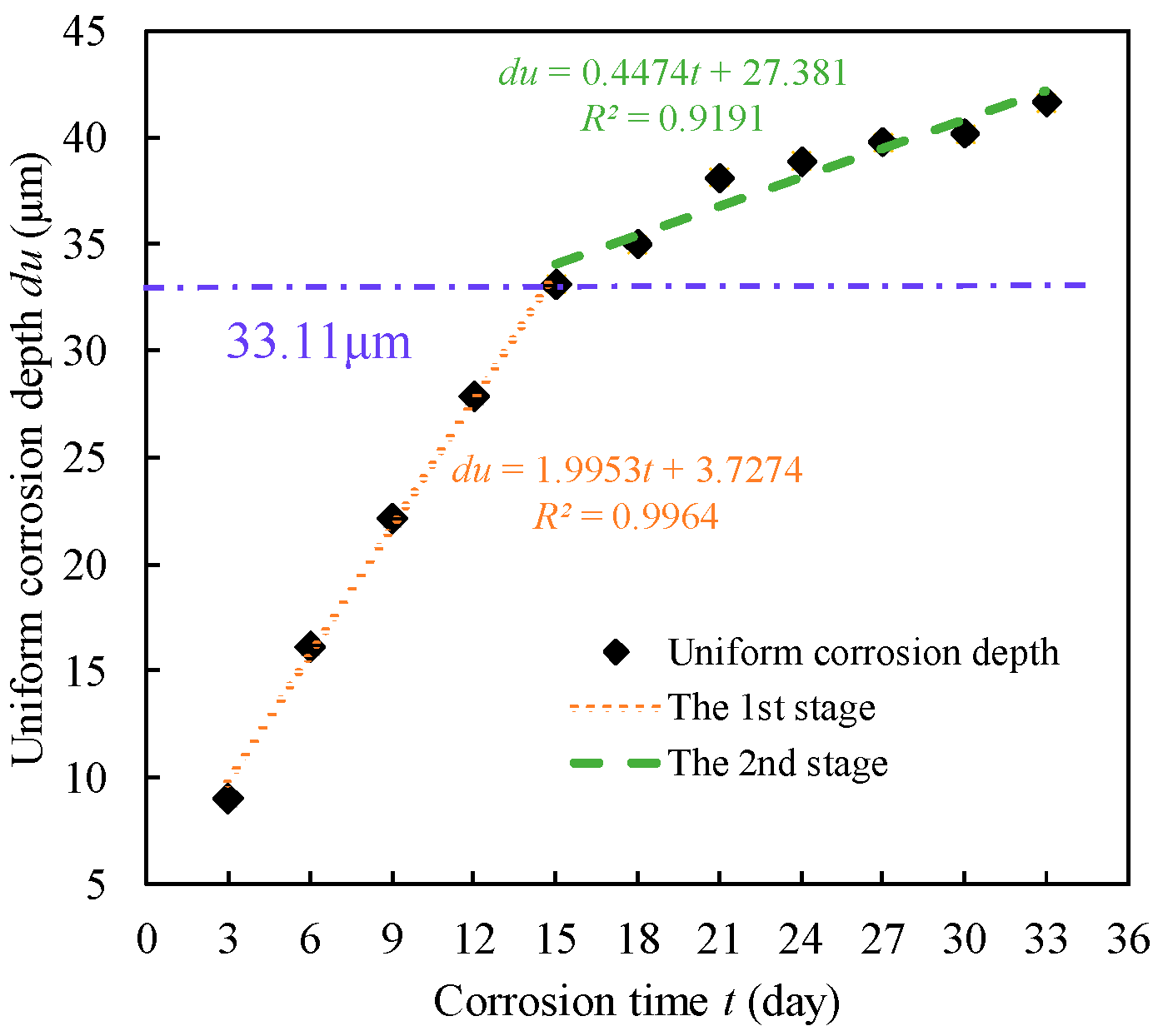
3.3.1. Calculation of Uniform Corrosion Depth

After reaching the predetermined corrosion duration, the target specimens are retrieved from the salt spray chamber, and chemical agents are employed to remove the rust deposits adhering to the surface of the wires. The calculation of the uniform corrosion depth was conducted using the mass loss analysis method. The mass of the wires was measured with an electronic balance with an accuracy of 0.001 g. The calculation method for the uniform corrosion depth is expressed as follows:

$$d_u(k,t)=\frac{\Delta \mathrm{m}(k,t)}{\rho A(k,t)}=\frac{\left[m(k,t_{init.})-m(k,t)\right]-\frac{1}{n}{\displaystyle {\sum }_{i=1}^n\left[m_{bc.}(i)-m_{ac}(i)\right]}}{\rho \pi D(k,t)L(k,t)}$$

(2)

where du(k,t)d represents the uniform corrosion depth of the k-th specimen after t days of accelerated salt spray corrosion testing. The density of the steel wire specimen is denoted by ρ. Δm(k,t) denoted the reasonable reduction in mass of the specimen after rust removal treatment. A(k,t) represents the surface area of the target specimen. m(k,t_init.) and m(k,t), respectively, represent the initial mass and the mass of the steel wire after rust removal. During the rust removal process, there may be a loss of mass from the steel wire substrate, which needs to be compensated for using $\frac{1}{n}{\displaystyle {\sum }_{i=1}^n\left[m_{bc}(i)-m_{ac}(i)\right]}$. n represents the total number of specimens to be treated. D(k,t) and L(k,t), respectively, represent the diameter and length of the k-th specimen.

Based on the detection results of Type Ⅰ corrosion specimens, the variation in steel wire corrosion depth with the corrosion specimens is shown in Figure 12. The corrosion depth gradually deepens with time, exhibiting a distinct two-stage characteristic. In the first stage, the corrosion depth increases rapidly, while in the second stage, the rate slows down, with a division point around 15 days. The corrosion process of the zinc coating on the steel wire is in the first stage, followed by the corrosion of the steel wire substrate, which corresponds to the second stage in the graph. Regression analysis of the data in the graph allows the average corrosion depth of the wire to be described as:

$$\left\{\begin{array}{c}{d}_{u,average}(t)=1.9953t+3.7274\\ d_{u,average}(t)=0.4474t+27.381\end{array}\right.$$

(3)

In order to establish the correspondence between the corrosion state of the steel wire in the accelerated salt spray corrosion test and the actual environmental corrosion conditions, this paper adopts the results of Marder’s outdoor corrosion test [43], based on which a correlation graph between the two is drawn, as shown in Figure 13. The bridge’s service area is located in a heavy industrial province. From this, it can be deduced that one day of salt spray testing is equivalent to corrosion occurring over 0.408 years in harsh industrial environments.

Figure 14 provides the correlation coefficients for the uniform corrosion depth of the steel wires in this experiment. The trend depicted in the figure indicates that from the initial stages, the variability of the uniform corrosion depth gradually decreases, ultimately reaching a stable state.

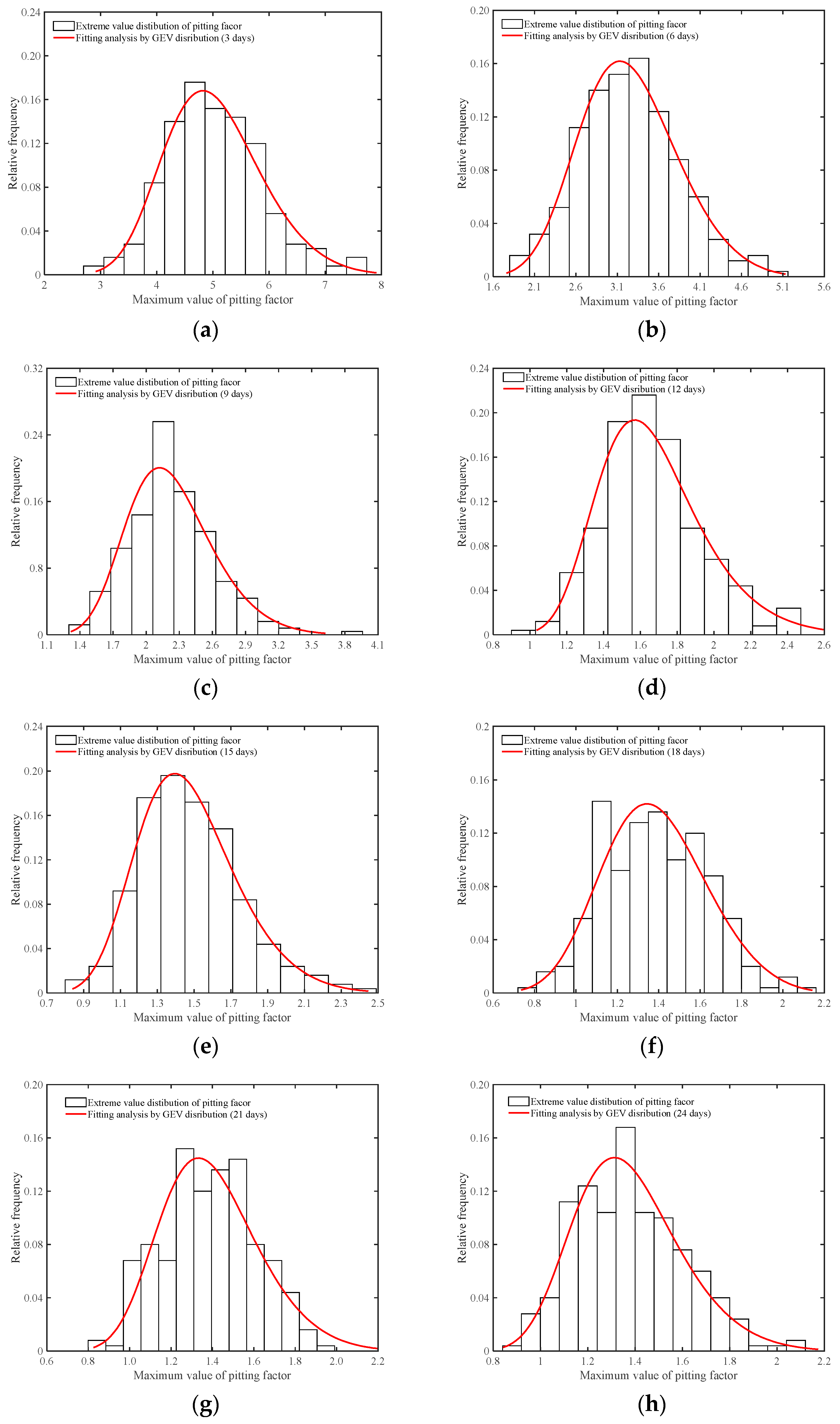
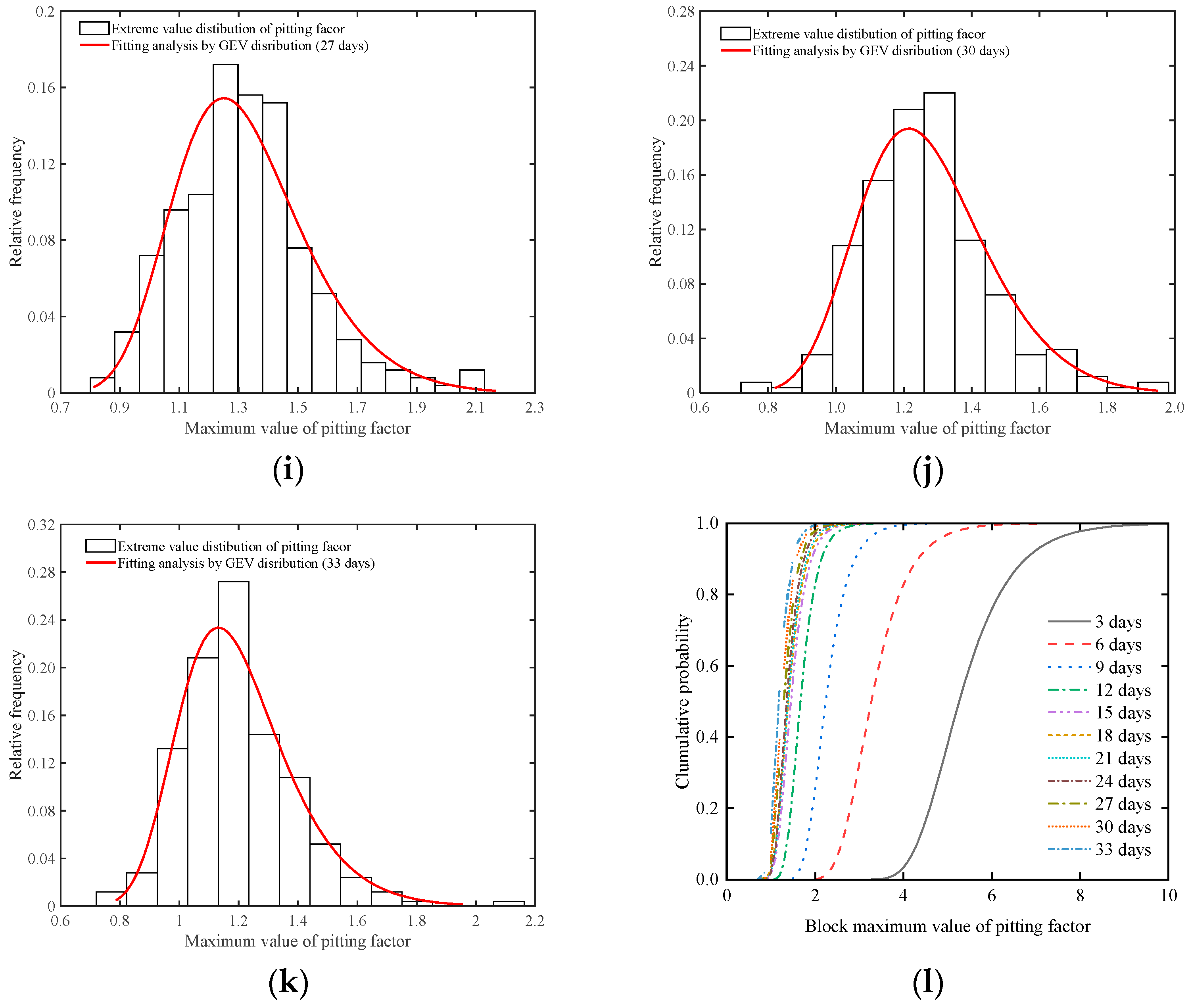
3.3.2. Extreme Value Modeling of Pitting Factors

In practical engineering, the inspection of corrosion states in bridge components is constrained by various factors, making comprehensive examinations infeasible. Through extreme value analysis, it becomes possible to establish a statistical model for the maximum pit depth in real-world applications. As the suspender of the arch bridge is in a vertical position during operation, the steel wires extracted exhibit minimal bending, allowing for the direct determination of pit depths with relative ease. After selecting sampling blocks on the target corroded steel wire and employing extreme value theory, the steel wire samples are subjected to extreme value modeling. The size of the sampling blocks in this study is 10 mm, meaning that along the length of the steel wire, a maximum pitting coefficient is recorded every 10 mm, forming a dataset of extreme values.

The Generalized Extreme Value distribution (GEV) is utilized for extreme value modeling of pitting coefficients in each sampling block. In this process, extreme value theory is employed as the theoretical foundation [44,45]. The cumulative distribution function (CDF) of the GEV distribution is given by:

$$Z_{\tau }~GEV(\mu ,\sigma ,\phi )=G(x;\mathsf{\Theta })=\exp \left\{-[1-\phi (\frac{x-\mu }{\sigma })\left.{]}^{\frac{1}{\phi }}\right\}\right.$$

(4)

To capture the variability of steel wire corrosion over time, a temporal parameter is introduced into Equation (4). The cumulative distribution expression of the extreme value distribution is then modified as follows:

$$Z_{p}GEV(\mu (t),\sigma (t),\xi (t))=G(x;\theta (t))=\left\{\begin{array}{c}\exp \left\{-[1-\xi (\frac{x-\mu (t)}{\sigma (t)})\left.{]}^{\frac{1}{\xi (t)}}\right\}\right.\xi (t)\ne 0\\ \exp \left\{-\exp [\frac{x-\mu (t)}{\sigma (t)}]\right\}\xi (t)\to 0\end{array}\right.$$

(5)

where μ, σ, and ξ denote the location parameter, scale parameter, and shape parameter, respectively. t denotes the corrosion time. For specimens at different corrosion time points, Figure 15a–k presents the fitting analysis results of the dynamic distribution of the GEV.

Figure 15l presents the cumulative probability density of the maximum pitting factor for specimens in each accelerated corrosion time segment. According to the modeling calculation results of Equation (5), the shape parameter ranges between −0.01706 and 0.0297, indicating that the shape parameter is near 0. This means that the maximum pitting factor samples from the sampling area can be described using a Type I extreme value distribution. Based on the two-stage characteristics revealed by the corrosion results of the steel wire, the fitting results of the unknown parameters and scale parameters of the Type I extreme value distribution can be obtained from Figure 16. It can be observed that in the first stage of corrosion development, the changes in the location and scale parameters of the Type I extreme value distribution follow an exponential decrease pattern, while during the second stage of corrosion development, the changes in the location parameter and scale parameter of the Type I extreme value distribution exhibit linear variations.

As the corrosion time increases, both the location parameter and scale parameter exhibit exponential decay during the first corrosion stage, following the pattern:

$$\left\{\begin{array}{c}\mu (t)=7.793\exp (-0.2408t)+1.199\begin{array}{c}\end{array}\\ \sigma (t)=1.157\exp (-0.2137t)+0.1994\end{array}\right.$$

(6)

Additionally, during the second corrosion stage, both the location parameter and scale parameter linearly decrease with the extension of corrosion time, conforming to the pattern:

$$\left\{\begin{array}{c}\mu (t)=-0.0151t+1.63\begin{array}{c}\end{array}\begin{array}{c}\end{array}\\ \sigma (t)=-0.0045t+0.3163\end{array}\right.$$

(7)

4. Variability of Spatial Corrosion of Steel Wires within Suspender Cross-Sections

4.1. Definition of Corrosion Process Discrepancy Factors

In this experiment, for a clear description of the experimental phenomena, the assumption of the shortest corrosion factor diffusion path was adopted. The steel wires located at different positions were stratified and numbered. In the experiment, starting from the simulated damage location, the stratification method for the Type II and Type III specimens is illustrated in Figure 17.

The corrosion process of Type II specimens simulates the condition where the protective layer of the suspenders has completely failed. To characterize the spatial variability of corrosion states among adjacent steel wires under unprotected conditions, the differential factor of the corrosion process can be defined as:

$$\delta ={\eta }_{i,j}/{\eta }_{i-1,k}$$

(8)

where δ denotes a random variable, denoting the differential factor among adjacent layers of corroded steel wires. η_i,j denotes the mass loss rate of the j-th wire in the i-th layer, while λ_i−1,k signifies the mass loss percentage of the kth wire in the (i − 1)-th layer. The mass loss rate for each wire can be determined as:

$$\eta =\frac{(m_{init.}-m_{corr.})}{m_{init.}}\times 100\%$$

(9)

where m_init. is the original steel wire mass and m_corr. is the steel wire mass after rust removal. It is noteworthy that when calculating the corrosion differential factor δ based on Equation (8), the j-th wire in the i-th layer is compared solely with its adjacent wires in terms of mass loss rates. Based on the wire layout shown in Figure 15a, it is apparent that the wires labeled “A” in the second layer are adjacent to the wires labeled “B”, “C”, and “D” in the first layer. Therefore, the mass loss rate of wire “A” needs to be compared with those of wires “B”, “C”, and “D” to obtain three samples of random variables.

For Type III specimens, to investigate the impact of corrosion time on specimens, examinations were conducted at three different time points. In this scenario, utilizing Equation (8) to describe the differences in sample corrosion processes would result in insufficient sample size for the random variable δ. To resolve this contradiction, the overall corrosion condition of each layer of steel wires in the simulated suspender specimens can be compared with the corrosion condition of the steel wires in the first layer. The differences in the corrosion states of the specimens will be redefined as:

$${\theta }_{i,j\to 1}={\stackrel{-}{\eta }}_{i,j}/{\stackrel{-}{\eta }}_{i,1}$$

(10)

In the equation, θ_i,j→1 denotes the overall corrosion level difference between the j-th layer wire of the i-th specimen and the first wire. η_i,j denotes the corrosion level of the j-th layer wire in the i-th specimen, calculated by the formula:

$${\stackrel{-}{\eta }}_{i,j}=\frac{1}{p_j}{\displaystyle \sum _{k_j=1}^{p_j}{\eta }_{i,j,k_j}}$$

(11)

In the equation, p_j denotes the total number of wires contained in the j-th layer of the simulated suspender specimen. λ_i,j,kj denotes the corrosion rate of the k-th steel wire in the i-th layer of the specimen, where k_j = 1,2, ⋯, p_j.

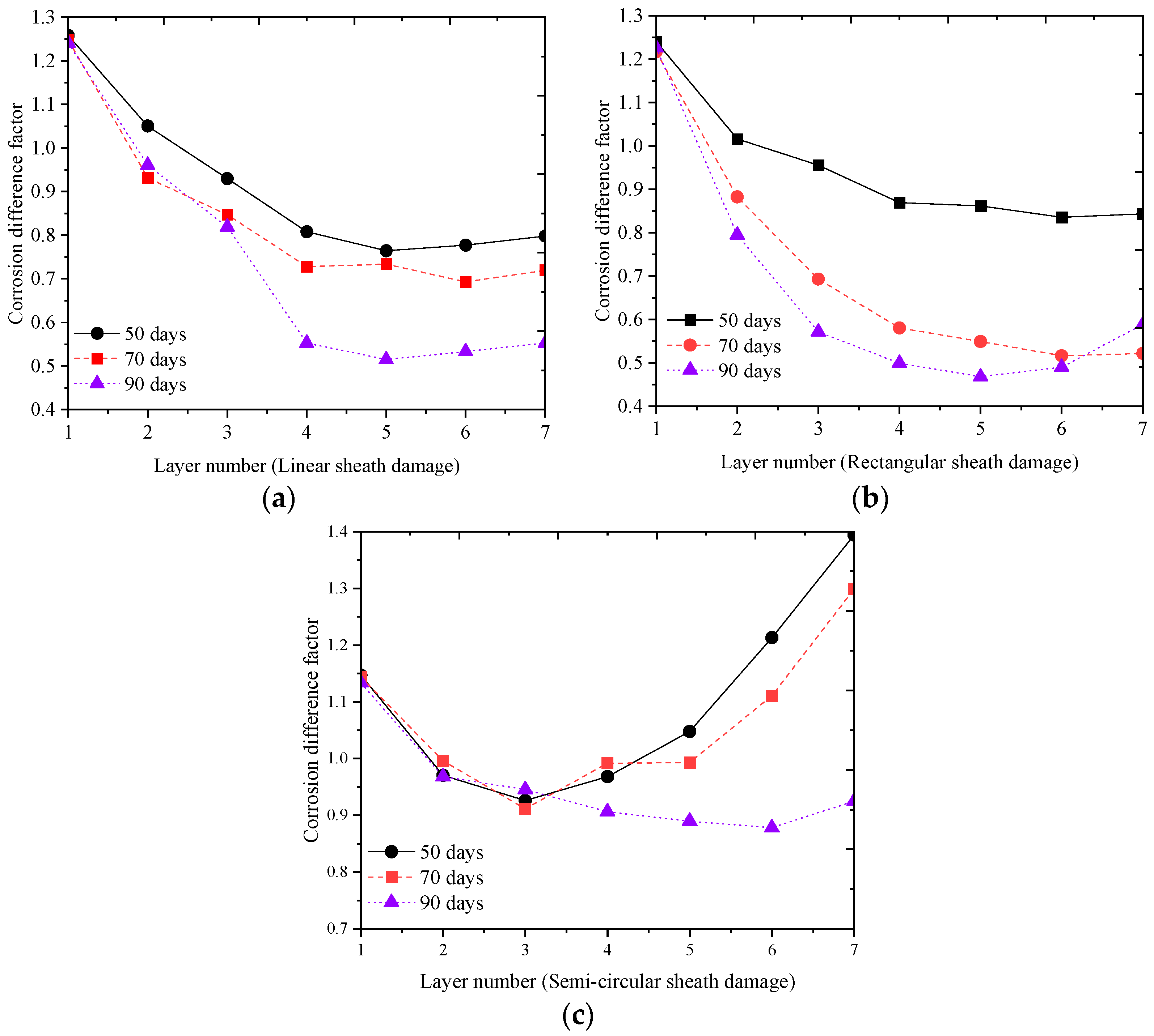
4.2. Analysis Results of the Sheath Damage Specimens

Taking the Type II specimen with a corrosion time of 90 days as an example, Figure 18 illustrates the macroscopic corrosion states of wires in each layer after specimen dissection. It is observed that the extent of corrosion decreases with the increase in the number of layers. The measured distribution of δ and the results of the fitting analysis are depicted in Figure 19. It can be noted that the differential factor in the corrosion process of adjacent layer wires can be described by a normal distribution, with mean and coefficient of variation values of 0.7074 and 0.3028, respectively.

For the type III of specimen, based on the analytical solution of Equations (10) and (11), the parameters of ${\theta }_{i,j\to 1}$ are presented in the line chart in Figure 20a–c. The findings demonstrate a pronounced influence of the shape of sheath damage on the spatial corrosion variability of steel wires within the suspender cross-section of arch bridges. With increasing corrosion time, the overall corrosion level difference between the layers of steel wires within the suspender decreases. The primary factors contributing to this phenomenon encompass the shape of sheath damage, the exposed surface area of the steel wires to the corrosive environment, and the deposition of corrosion by-products. It is evident that the process of corrosion erosion of the steel wire in the corrosive environment is significantly influenced by the shape of the sheath damage.

Among the three different sheath damage specimens, the wire samples with rectangular sheath damage and linear sheath damage exhibit stronger spatial corrosion variability compared to those with semi-circular damages. The genesis of this phenomenon is attributed to the hindering effect of sheath damage on the diffusion of corrosion factors. In certain circumstances, the corrosion severity of the innermost steel wires exceeds that of the outer layers, attributable to the heightened propensity for corrosion factor accumulation within the internal wire environment, ultimately impeding their diffusion and dilution.

5. Conclusions

Through conducting accelerated corrosion tests using three different types of specimens in acetic acid salt spray, the study investigated the corrosion development process of high-strength steel wires inside the suspender, surface morphology changes, the temporal evolution model of pitting corrosion on steel wires, and the spatial corrosion variability of steel wires under different states of damage to the suspender protective covering. The following conclusions can be drawn from the present research:

(1)

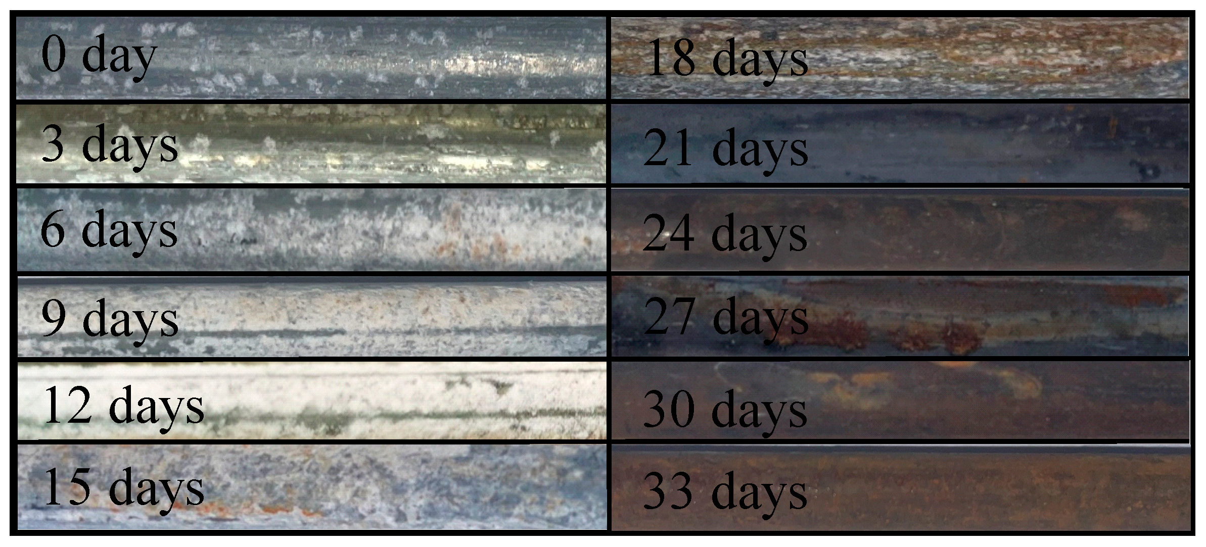
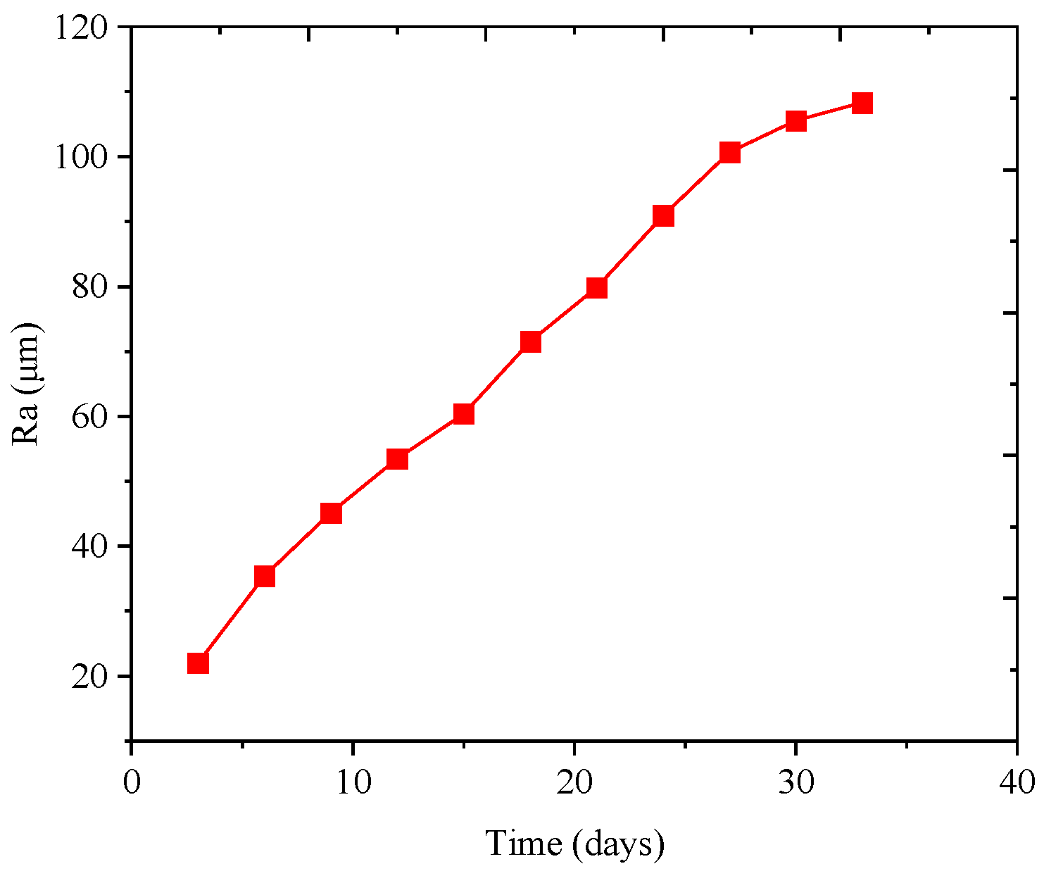
The galvanized layer of the steel wire undergoes initial oxidation, leading to the formation of white oxide. Upon infiltration of corrosion factors from the environment into the steel wire substrate, yellow oxide subsequently appears. Finally, the steel wire surface becomes entirely covered by red iron oxide. The surface roughness (Ra) of suspender wires exhibits a strong linear positive correlation with the average corrosion depth, indicating that the roughness of corroded wires increases with the degree of corrosion.

(2)

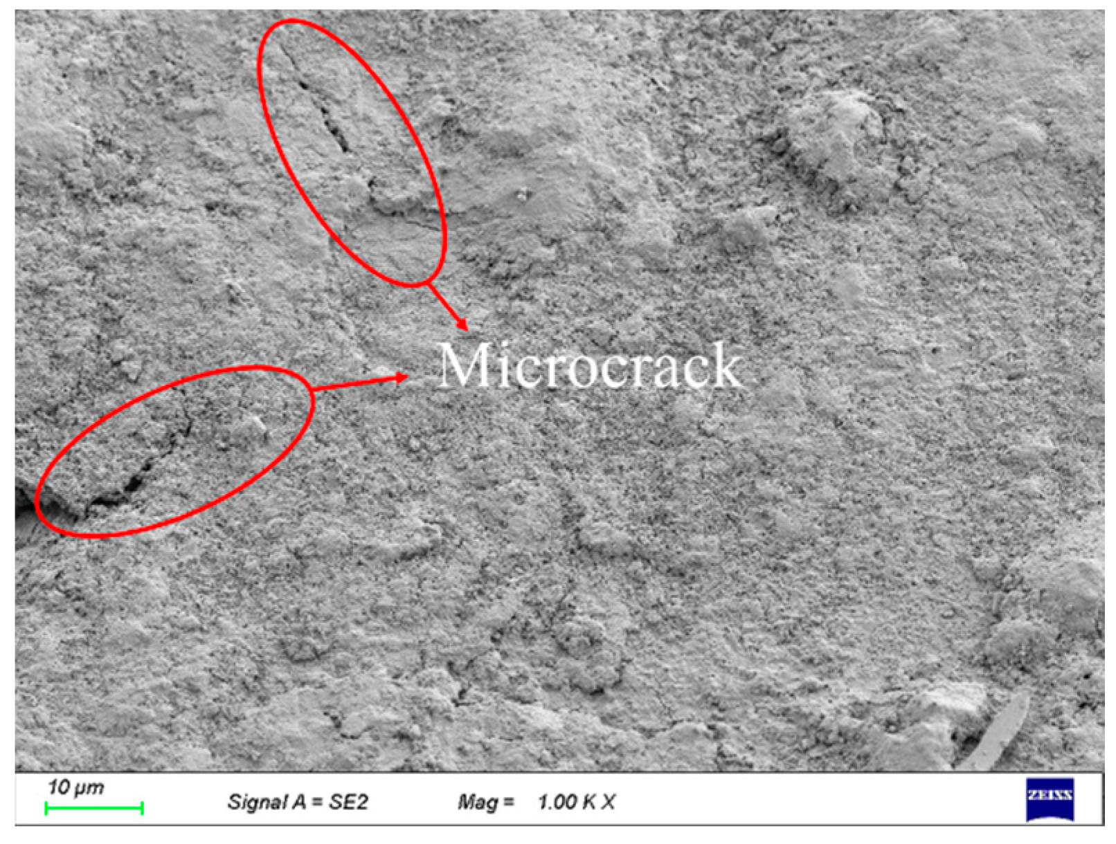
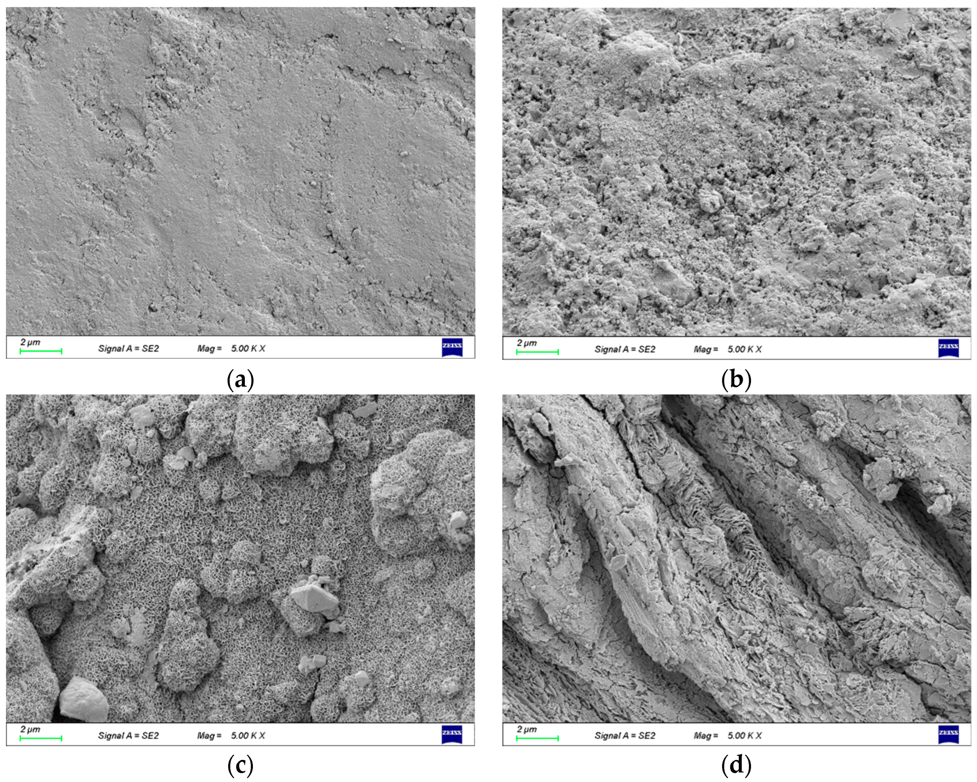
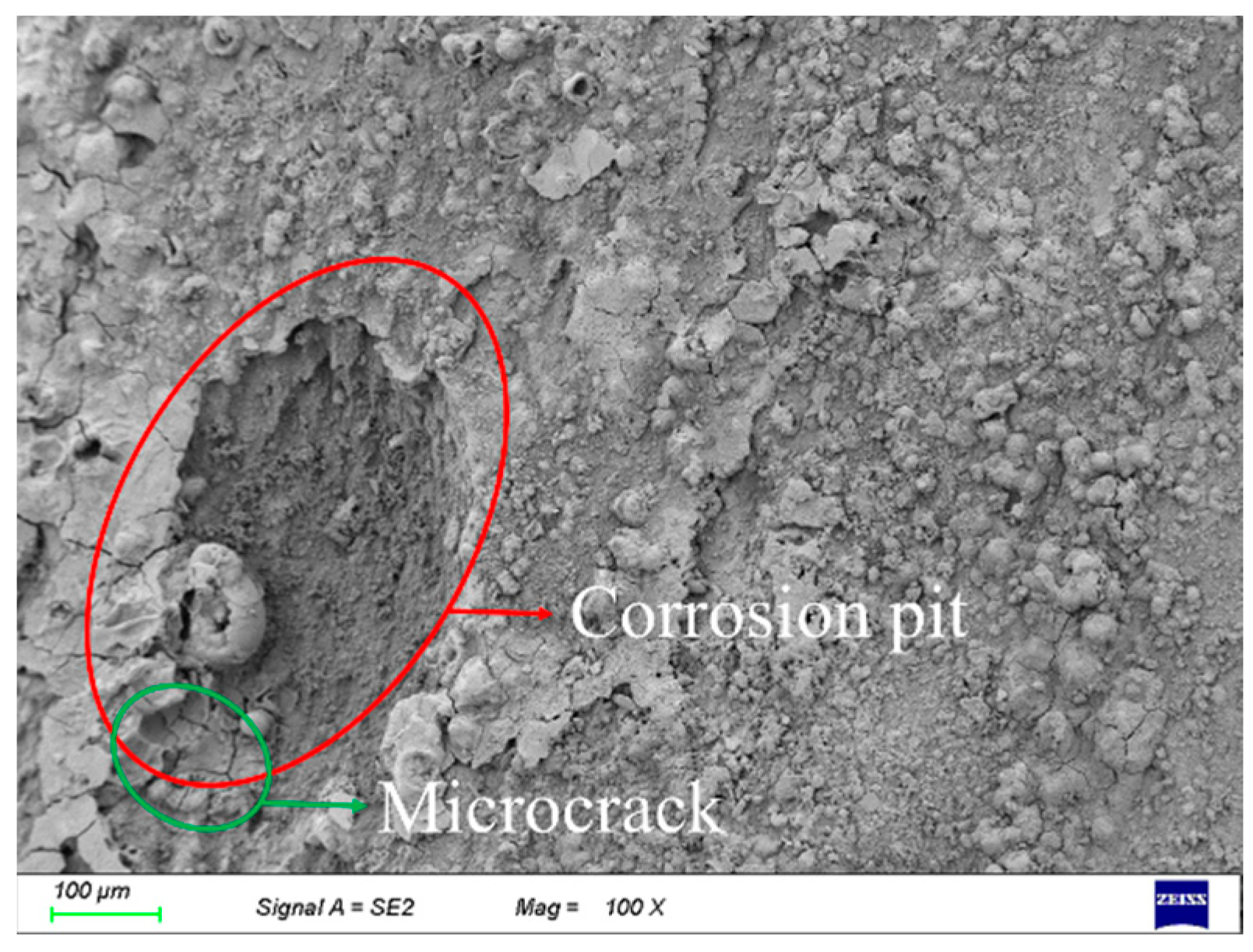
Throughout the entire corrosion process, the microscopic structure of the steel wire surface transitions from a dense structure to a porous one. Corrosion of the steel wire substrate results in the accumulation of granular and fluffy corrosion products. With prolonged corrosion time, heavily corroded steel wire surfaces exhibit a stacked flake-like deposition of corrosion products. The generation of steel wire cracks accompanies the entire process of corrosion development.

(3)

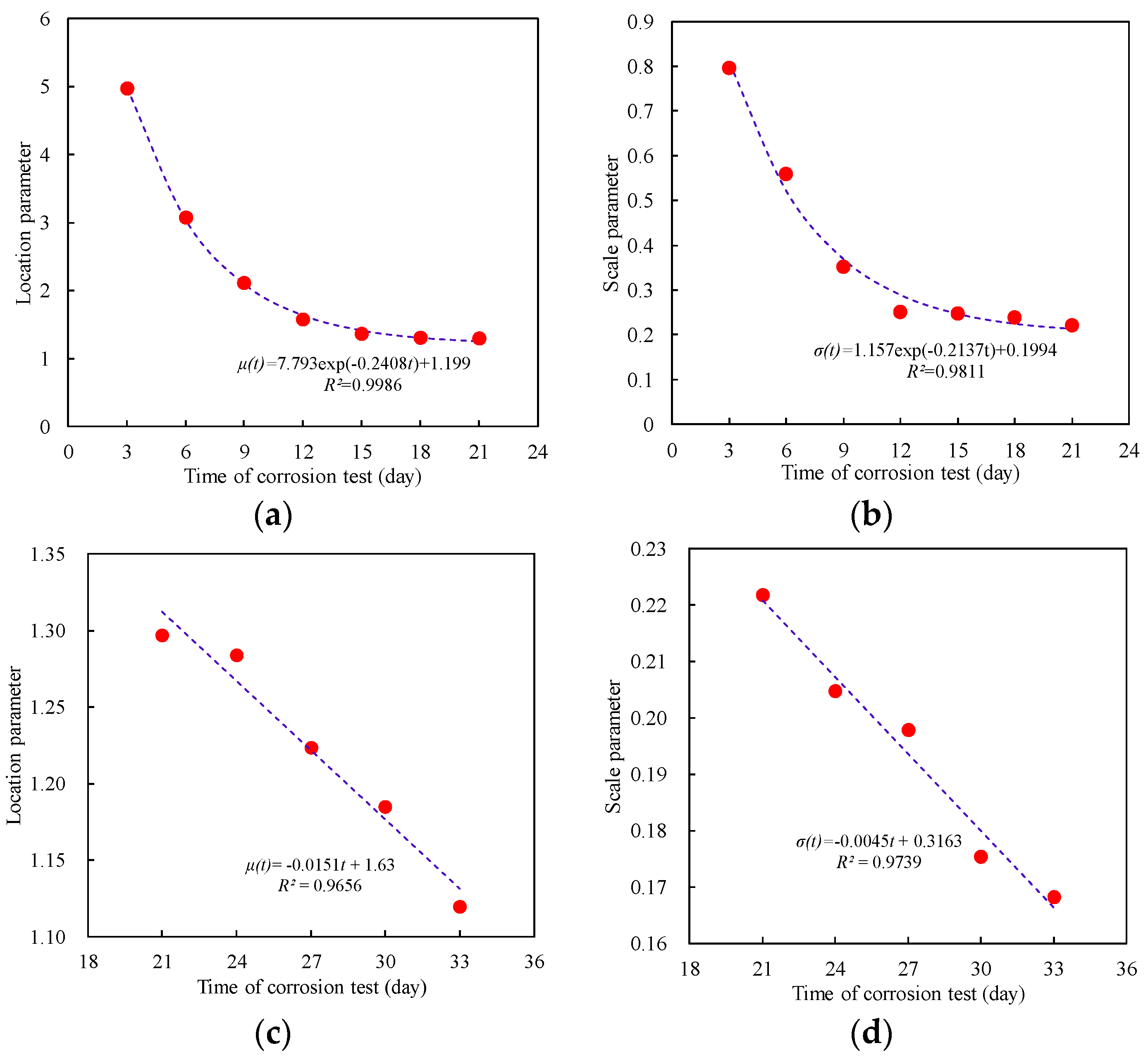
A dynamic generalized extreme value distribution is employed to establish a time-varying model for the point corrosion of corroded wires. Location and scale parameters exhibit exponential and linear decreases, respectively, in the first corrosion stage, followed by linear declines in the second corrosion stage.

(4)

Under accelerated corrosion for 90 days, the coefficient of variation in the corrosion process between adjacent layers within the suspender wire bundle specimens with protective measures failure follows a normal distribution, with a mean of 0.7074 and a coefficient of variation of 0.3028.

(5)

The state of protective layer damage significantly influences the corrosion status of wires within suspenders. With increasing corrosion time, the differences in the corrosion extent of wires in different layers gradually diminish. Based on the above research, it can provide a certain reference for the assessment of the service life of the suspenders.

References

1. Deng, Y.; Deng, L. Suspender Replacement Method for Long-Span Concrete-Filled Steel Tubular Arch Bridges and Cable Force Measurement Based on Frequency Method. Adv. Civ. Eng. 2021, 2021, 1–21. [Google Scholar] [CrossRef]
2. Li, S.; Zhang, L.; Wang, Y.; Hu, P.; Jiang, N.; Guo, P.; Wang, X.; Feng, H. Effect of cathodic protection current density on corrosion rate of high-strength steel wires for stay cable in simulated dynamic marine atmospheric rainwater. Structures 2021, 29, 1655–1670. [Google Scholar] [CrossRef]
3. Li, F.; Liu, Z.; Zhao, Y.; Qu, Y.; Lu, R. Experimental study on corrosion progress of interior bond section of anchor cables under chloride attack. Constr. Build. Mater. 2014, 71, 344–353. [Google Scholar] [CrossRef]
4. Sun, H.; Xu, J.; Chen, W.; Yang, J. Time-Dependent Effect of Corrosion on the Mechanical Characteristics of Stay Cable. J. Bridg. Eng. 2018, 23, 04018019. [Google Scholar] [CrossRef]
5. Li, D.; Zhou, Z.; Ou, J. Dynamic behavior monitoring and damage evaluation for arch bridge suspender using GFRP optical fiber Bragg grating sensors. Opt. Laser Technol. 2012, 44, 1031–1038. [Google Scholar] [CrossRef]
6. Liu, P.; Lu, H.; Chen, Y.; Zhao, J.; An, L.; Wang, Y.; Liu, J. Fatigue Analysis of Long-Span Steel Truss Arched Bridge Part II: Fatigue Life Assessment of Suspenders Subjected to Dynamic Overloaded Moving Vehicles. Metals 2022, 12, 1035. [Google Scholar] [CrossRef]
7. Miao, C.; Yu, J.; Mei, M. Distribution law of corrosion pits on steel suspension wires for a tied arch bridge. Anti-Corrosion Methods Mater. 2016, 63, 166–170. [Google Scholar] [CrossRef]
8. Suzumura, K.; Nakamura, S.-I. Environmental Factors Affecting Corrosion of Galvanized Steel Wires. J. Mater. Civ. Eng. 2004, 16, 1–7. [Google Scholar] [CrossRef]
9. Wu, S.; Chen, H.; Ramandi, H.L.; Hagan, P.C.; Crosky, A.; Saydam, S. Effects of environmental factors on stress corrosion cracking of cold-drawn high-carbon steel wires. Corros. Sci. 2018, 132, 234–243. [Google Scholar] [CrossRef]
10. Chen, A.; Yang, Y.; Ma, R.; Li, L.; Tian, H.; Pan, Z. Experimental study of corrosion effects on high-strength steel wires considering strain influence. Constr. Build.Mater. 2020, 240, 117910. [Google Scholar] [CrossRef]
11. Li, S.; Xu, Y.; Li, H.; Guan, X. Uniform and Pitting Corrosion Modeling for High-Strength Bridge Wires. J. Bridg. Eng. 2014, 19, 04014025. [Google Scholar] [CrossRef]
12. Li, S.; Xu, Y.; Zhu, S.; Guan, X.; Bao, Y. Probabilistic deterioration model of high-strength steel wires and its application to bridge cables. Struct. Infrastruct. Eng. 2014, 11, 1240–1249. [Google Scholar] [CrossRef]
13. Karanci, E.; Betti, R. Modeling Corrosion in Suspension Bridge Main Cables. I: Annual Corrosion Rate. J. BridgeEng. 2018, 23, 4018025. [Google Scholar] [CrossRef]
14. Xue, S.; Shen, R.; Xue, H.; Zhu, X.; Wu, Q.; Zhang, S. Failure analysis of high-strength steel wire under random corrosion. Structures 2021, 33, 720–727. [Google Scholar] [CrossRef]
15. Xu, Y.; Li, H.; Li, S.; Guan, X.; Lan, C. 3-D modelling and statistical properties of surface pits of corroded wire based on image processing technique. Corros. Sci. 2016, 111, 275–287. [Google Scholar] [CrossRef]
16. Fang, K.; Li, S.; Chen, Z.; Li, H. Geometric characteristics of corrosion pits on high-strength steel wires in bridge cables under applied stress. Struct. Infrastruct. Eng. 2020, 17, 34–48. [Google Scholar] [CrossRef]
17. Li, R.; Miao, C.; Wei, T. Experimental study on corrosion behaviour of galvanized steel wires under stress. Corros. Eng. Sci. Technol. 2020, 55, 622–633. [Google Scholar] [CrossRef]
18. Li, R.; Miao, C.; Feng, Z.; Wei, T. Experimental study on the fatigue behavior of corroded steel wire. J. Constr. Steel Res. 2021, 176, 106375. [Google Scholar] [CrossRef]
19. Wang, Y.; Zhang, W.; Zheng, Y. Experimental Study on Corrosion Fatigue Performance of High-Strength Steel Wire with Initial Defect for Bridge Cable. Appl. Sci. 2020, 10, 2293. [Google Scholar] [CrossRef]
20. Jiang, J.H.; Ma, A.B.; Weng, W.F.; Fu, G.H.; Zhang, Y.F.; Liu, G.G.; Lu, F.M. Corrosion fatigue performance of pre-split steel wires for high strength bridge cables. Fatigue Fract. Eng. Mater. Struct. 2009, 32, 769–779. [Google Scholar] [CrossRef]
21. Rajasankar, J.; Iyer, N.R. A probability-based model for growth of corrosion pits in aluminum alloys. Eng. Fract.Mech. 2006, 73, 1149–1150. [Google Scholar] [CrossRef]
22. Jones, K.; Hoeppner, D.W. Pit-to-crack transition in pre-corroded 7075-T6 aluminum alloy under cyclic loading. Corros. Sci. 2005, 47, 2185–2198. [Google Scholar] [CrossRef]
23. Liu, Z.; Guo, T.; Yu, X.; Huang, X.; Correia, J. Corrosion fatigue and electrochemical behaviour of steel wires used in bridge cables. Fatigue Fract. Eng. Mater. Struct. 2021, 44, 63–73. [Google Scholar] [CrossRef]
24. Zheng, X.; Xie, X.; Li, X. Experimental Study and Residual Performance Evaluation of Corroded High-Tensile Steel Wires. J. Bridg. Eng. 2017, 22, 04017091. [Google Scholar] [CrossRef]
25. Jiang, C.; Wu, C.; Jiang, X. Experimental study on fatigue performance of corroded high-strength steel wires used in bridges. Constr. Build. Mater. 2018, 187, 681–690. [Google Scholar] [CrossRef]
26. Li, H.; Lan, C.M.; Ju, Y.; Li, D.S. Experimental and Numerical Study of the Fatigue Properties of Corroded Parallel Wire Cables. J. Bridg. Eng. 2012, 17, 211–220. [Google Scholar] [CrossRef]
27. Lan, C.; Xu, Y.; Liu, C.; Li, H.; Spencer, B. Fatigue life prediction for parallel-wire stay cables considering corrosion effects. Int. J. Fatigue 2018, 114, 81–91. [Google Scholar] [CrossRef]
28. Wang, G.; Ma, Y.; Wang, L.; Zhang, J. Experimental study and residual fatigue life assessment of corroded high-tensile steel wires using 3D scanning technology. Eng. Fail. Anal. 2021, 124, 105335. [Google Scholar] [CrossRef]
29. Deng, Y.; Deng, L. Corrosion Fatigue Test and Performance Evaluation of High-Strength Steel Wires Based on the Suspender of a 11-Year-Old Concrete-Filled Steel Tube Arch Bridge. Coatings 2022, 12, 1475. [Google Scholar] [CrossRef]
30. Wang, Y.; Zheng, Y.Q.; Zhang, W.H.; Lu, Q.R. Damage evolution simulation and life prediction of high-strength steel wire under the coupling of corrosion and fatigue. Corros.Sci. 2020, 164, 108368. [Google Scholar]
31. Co, N.E.C.; Burns, J.T. Effects of macro-scale corrosion damage feature on fatigue crack initiation and fatigue behavior. Int. J. Fatigue 2017, 103, 234–247. [Google Scholar] [CrossRef]
32. Sun, B. A continuum model for damage evolution simulation of the high strength bridge wires due to corrosion fatigue. J. Constr. Steel Res. 2018, 146, 76–83. [Google Scholar] [CrossRef]
33. Wang, Y.; Zheng, Y.; Zhang, W.; Lu, Q. Analysis on damage evolution and corrosion fatigue performance of high-strength steel wire for bridge cable: Experiments and numerical simulation. Theor. Appl. Fract. Mech. 2020, 107, 102571. [Google Scholar] [CrossRef]
34. Miao, C.; Li, R.; Yu, J. Effects of characteristic parameters of corrosion pits on the fatigue life of the steel wires. J. Constr. Steel Res. 2020, 168, 105879. [Google Scholar] [CrossRef]
35. Chen, C.; Jie, Z.; Wang, K. Fatigue life evaluation of high-strength steel wires with multiple corrosion pits based on the TCD. J. Constr. Steel Res. 2021, 186, 106913. [Google Scholar] [CrossRef]
36. Sloane, M.J.D.; Betti, R.; Marconi, G.; Hong, A.L.; Khazem, D. Experimental Analysis of a Nondestructive Corrosion Monitoring System for Main Cables of Suspension Bridges. J. Bridg. Eng. 2013, 18, 653–662. [Google Scholar] [CrossRef]
37. Xia, R.; Zhang, H.; Zhou, J.; Liao, L.; Zhang, Z.; Yang, F. Probability evaluation method of cable corrosion degree based on self-magnetic flux leakage. J. Magn. Magn. Mater. 2021, 522, 167544. [Google Scholar] [CrossRef]
38. Karthik, M.M.; Terzioglu, T.; Hurlebaus, S.; Hueste, M.B.; Weischedel, H.; Stamm, R. Magnetic flux leakage technique to detect loss in metallic area in external post-tensioning systems. Eng. Struct. 2019, 201, 109765. [Google Scholar] [CrossRef]
39. Kazuhiro, M.; Marios, C.; Shunichi, N. Experimental assessment of the fatigue strength of corroded bridge wires using non-contact mapping techniques. Corros. Sci. 2021, 178, 109047. [Google Scholar]
40. International Organization for Standardization. Corrosion Tests in Artificial Atmosphere Salt Spray Tests; HIS under license with ISO; International Organization for Standardization: Geneva, Switzerland, 1990; p. 9227. [Google Scholar]
41. International Organization for Standardization. Corrosion of Metals and Alloys-Removal of Corrosion Products from Corrosion Test Specimens; HIS under llicense with ISO; International Organization for Standardization: Geneva, Switzerland, 1991; p. 8407. [Google Scholar]
42. Xue, S.; Shen, R.; Chen, W.; Miao, R. Corrosion fatigue failure analysis and service life prediction of high strength steel wire. Eng. Fail. Anal. 2020, 110, 104440. [Google Scholar] [CrossRef]
43. Marder, A. The metallurgy of zinc-coated steel. Prog. Mater. Sci. 2000, 45, 191–271. [Google Scholar] [CrossRef]
44. Yuan, Y.; Han, W.; Li, G.; Xie, Q.; Guo, Q. Time-dependent reliability assessment of existing concrete bridges including non-stationary vehicle load and resistance processes. Eng. Struct. 2019, 197, 109426. [Google Scholar] [CrossRef]
45. Benstock, D.; Cegla, F. Sample selection for extreme value analysis of inspection data collected from corroded surfaces. Corros. Sci. 2016, 103, 206–214. [Google Scholar] [CrossRef]
Figure 1. Salt spray test equipment. (a) Salt spray chamber, (b) Air compressor.
Coatings 14 00628 g001
Figure 2. Corrosion test wire specimens. (a) The Single Steel Wire Specimen, (b) Protection failure specimen, (c) Strip-shaped Damage, (d) square block damage, (e) semi-circular damage.
Coatings 14 00628 g002
Figure 3. Rust removal of a single steel wire specimen. (a) Corroded steel wire original appearance, (b) Derusting with hydrochloric acid, (c) De-rusting with steel wire.
Coatings 14 00628 g003
Figure 4. Macroscopic surface of corroded steel wire.
Coatings 14 00628 g004
Figure 5. Field emission scanning electron microscope.
Coatings 14 00628 g005
Figure 6. Incipient Crack Formation on the Steel Wire Surface.
Coatings 14 00628 g006
Figure 7. The evolution of the microscopic state on the surface of the steel wire. (a) Initial appearance; (b) 10 days; (c) 21 days; (d) 31 days.
Coatings 14 00628 g007
Figure 8. Surface Corrosion Pits and Cracks in Corroded Steel Wire.
Coatings 14 00628 g008
Figure 9. Confocal Laser Scanning Microscope.
Coatings 14 00628 g009
Figure 10. Laser microscope scanning results. (a) Initial appearance-3D, (b) Initial appearance-2D, (c) 10 days-3D, (d) 10 days-2D, (e) 21 days-3D, (f) 21 days-2D, (g) 31 days-3D, (h) 31 days-2D.
Coatings 14 00628 g010aCoatings 14 00628 g010b
Figure 11. The relationship between roughness and time.
Coatings 14 00628 g011
Figure 12. Uniform corrosion depth.
Coatings 14 00628 g012
Figure 13. Corrosion-Time Conversion Relationship.
Coatings 14 00628 g013
Figure 14. Correlation coefficient of uniform corrosion depth.
Coatings 14 00628 g014
Figure 15. Analyzing pitting factor extremes with the GEV distribution method. (a) Accelerated corrosion for 3 days; (b) Accelerated corrosion for 6 days; (c) Accelerated corrosion for 9 days; (d) Accelerated corrosion for 12 days; (e) Accelerated corrosion for 15 days; (f) Accelerated corrosion for 18 days; (g) Accelerated corrosion for 21 days; (h) Accelerated corrosion for 24 days (i) Accelerated corrosion for 27 days; (j) Accelerated corrosion for 30 days; (k) Accelerated corrosion for 33 days; (l) Cumulative maximum value of pitting factor.
Coatings 14 00628 g015aCoatings 14 00628 g015b
Figure 16. Variation in distribution parameters of Type I extreme value distribution. (a) Location parameter of the first stage; (b) Scale parameter of the first stage; (c) Location parameter of the second stage; (d) Scale parameter of the second stage.
Coatings 14 00628 g016
Figure 17. Schematic Diagram of Layered Configuration for Steel Wire Specimens. (a) Protection failure specimen; (b) Linear sheath damage; (c) Rectangular sheath damage; (d) Semi-circular sheath damage.
Coatings 14 00628 g017
Figure 18. Corrosion morphology of wires.
Coatings 14 00628 g018
Figure 19. Normal distribution fitting analysis.
Coatings 14 00628 g019
Figure 20. Differential Analysis of Corrosion Process Considering Sheath Damage. (a) Linear sheath damage; (b) Rectangular sheath damage; (c) Semi-circular sheath damage.
Coatings 14 00628 g020