A Multi-Parameter-Coupled Mixed Lubrication Model for Rolling Interface Analysis: An Investigation on Interfacial Oil Pressure and Oil Film Thickness

Abstract

Utilizing the average Reynolds equation, lubrication friction theory, metal rolling deformation theory, and temperature energy theory, a multi-parameter-coupling mixed lubrication model considering the influence of surface roughness with Gaussian distribution characteristics under rolling conditions was established. The results show that the stress distribution of the lubricating oil at the rolling interface conforms to the typical characteristics of line contact stress distribution. The oil film pressure does not increase significantly with the increase in the reduction ratio. A second peak pressure appears before the outlet. The second peak pressure reaches its maximum when ε = 0.2. The rolling speed has little effect on oil film pressure, but greatly affects oil film thickness. The influence of rolling speed mainly occurs in the outlet zone and at the second peak pressure location. The oil film thickness increases with rolling speed. During rolling, the temperature rise in the rolls exhibits two peak values. The first peak appears near the neutral point, and the second peak appears near the outlet, which is also where the second peak pressure is located. The influence of temperature will reduce the peak stress on the rolls. The overall stress on the rolls will also decrease.

1. Introduction

Rolling is currently the most important metal forming process, with approximately 70% of metal production processes involving rolling. Lubrication in cold rolling plays a crucial role in metal forming processes by providing a lubricating oil film between the workpiece and the rolls, which prevents severe metal-to-metal contact and resulting wear. The main sources of heat in the rolling process, such as deformation heat of the strip and frictional heat at the rolling interface, cause changes in the temperature of the rolls, which have a significant impact on the stability of the rolling process and the quality of the strip. The temperature at the rolling interface, the friction coefficient, the oil film thickness, and the deformation of the metal strip are all interconnected. Changes in the temperature at the rolling interface during the metal deformation process can alter the viscosity of the lubricating oil, resulting in changes in the oil film thickness, which in turn affects the friction coefficient. This leads to variations in the generated frictional heat, ultimately influencing the temperature at the rolling interface [1,2,3].

Most of the rough surfaces of rolls follow a Gaussian distribution. Christensen used a polynomial function to approximate the Gaussian density function and proposed a stochastic model for frictional lubrication on rough surfaces based on probability statistics theory. Many scholars have used this model to study the influence of surface roughness on the performance of frictional lubrication contact surfaces [4]. Masijedi analyzed and calculated the inlet oil film thickness under mixed conditions in the entry of rolling, introducing a mixed-state rolling model [5]. Based on this model and the information about the Gaussian height distribution of the workpiece and roll surfaces, the actual contact area can be estimated. Further improvements were made by considering the effects of the inlet oil film thickness and the thermal hardening of the rolling metal. Kimura modeled the lubrication state at the rolling interface and analyzed the influence of roughness on the entry region of rolling [6]. LO simplified the mixed lubrication model and analyzed the influence of roughness on the deformation work zone of the workpiece [7]. Hao developed a Reynolds equation-based model under various simplifications and assumptions, which described three different regions in the rolling process: the entry region, transition region, and work region [8]. Akbarzadeh discussed mixed lubrication in low-speed rolling, where the pressure generated in the entry region can be neglected [9]. The above studies have shown that higher fluid pressure can be generated in the work region due to wedge action, and empirical evidence suggests that fluid dynamic effects still exist under low-speed conditions. This helps to better understand the lubrication in the rolling process.

The finite difference method has been widely used in the study of heat transfer, and it has also become one of the main methods for calculating the temperature field and thermal deformation of rolling mills in mechanical engineering. This method involves discretizing the continuous solution domain into discrete grid points and approximating the derivatives using difference quotients and integrals using numerical approximations. Subsequently, a set of finite difference equations corresponding to the governing differential equations is established for numerical solution. The finite difference equations for the temperature field of rolling mills can be directly derived from the principle of energy conservation, or by replacing the differential terms in the heat conduction differential equation derived from the principle of energy conservation with difference quotients [10]. Representative studies include the work of Hiroshi Yanzaki in 1974, where they derived the finite difference equations for the temperature field of rolling mills from the perspective of energy conservation [11]. Yamaguchi S. developed a numerical simulation model based on the finite difference method to predict the temperature field and thermal deformation of rolling mills, surpassing the traditional method of rolling mill lateral movement, by calculating the amount of thermal deformation in the contact area using a fixed cycle and step size [12]. Li constructed boundary conditions for the rolling area, non-rolling area, shoulder, neck, and end of the rolling mill that closely matched the actual conditions, and used the finite difference method to calculate the two-dimensional temperature distribution, obtaining the variation patterns of temperature distribution and thermal deformation with a diameter [13]. These studies demonstrate the effectiveness of the finite difference method in approximating and solving the temperature field and thermal deformation of rolling mills, providing valuable insights for the understanding and control of the rolling process in mechanical engineering. However, in these studies, the surface of the rolling strip is approximated as smooth, without considering the impact of surface roughness, and the amplitude of the roughness can affect the lubrication status of the interface, and the physical properties of lubricating oil under different temperatures can show significant differences. It can be seen from the studies of scholars that the environment in which the rolls are located is highly complex, and the determination of thermal boundary conditions is difficult. The study of the rolling interface conditions considering the coupling of the temperature field, flow field, and structural field has always been a weak link in roll profile research.

The author constructed a coupled model of rolling temperature characteristics and lubricant viscous properties for metal rolling, considering the surface roughness of the rolled workpiece to follow a Gaussian distribution, the lubricant flow to be described by the Reynolds equation, the deformation of the rolled workpiece by the law of constant volume, and the thermal deformation of the rolled workpiece by the temperature energy equation. The model describes the viscous properties of the lubricant in the rolling zone and analyzes the oil film pressure and oil film thickness under different reduction ratios and rolling speeds. The research results of this study help to establish a theoretical basis for describing the dynamic frictional behavior at the rolling interface and analyzing the stability of rolling processes.

2. Modeling of Roughness at the Rolling Interface

In early studies on rolling lubrication mechanisms, it was often assumed that the surfaces of the rolls and strip were smooth, which is not the case in actual production. In order to establish a more realistic and accurate mathematical model for calculation, the influence of strip roughness on the flow of lubricant in the rolling work interface must be taken into account. In reality, both the strip and roll surfaces are uneven, with surface peaks and valleys that are randomly distributed, as shown in Figure 1.

According to the Christensen theory of random roughness distribution, the surface roughness of both the strip and the roll in the rolling process follows a Gaussian distribution [4]. The probability density function (PDF) of the Gaussian surface is denoted as $P_G$, and it can be expressed as:

$$P_G\left(\tau \right)=\frac{\mathit{exp}\left[-{\tau }^2/\left(2R_q^2\right)\right]}{R_q\sqrt{2\pi }}$$

(1)

In Equation (1), $\tau$ represents the average values of ${\tau }_1$ and ${\tau }_2$, and $R_q$ denotes the root mean square (RMS) value, which represents the numerical value of the roughness of the rolled piece surface.

$$R_q=\sqrt{\frac{1}{L}{\int }_0^L{g}^{2}dx}$$

(2)

In Equation (2), $x$ represents the coordinate along the measurement direction, $g$ denotes the local amplitude of the surface measured from the mean line, and $L$ represents the length of the measurement area.

The probability density of the Gaussian distribution can be represented by a polynomial function, $P_C$, as follows:

$$P_C\left(\tau \right)=\left\{\begin{array}{c}\frac{35}{96R_q^2}{\left[1-\frac{1}{9}{\left(\frac{\tau }{R_q}\right)}^2\right]}^3 \\ 0,\left|\tau \right|>3R_q\end{array}\right.,\left|\tau \right|\le 3R_q$$

(3)

The spacing between the surface roughness profiles of the rolled piece can be represented by the autocorrelation function, $\varphi$ [14]:

$$\varphi \left(\alpha \right)=\mathit{exp}\left(-\frac{\alpha }{{\alpha }^{*}}\right)$$

(4)

The autocorrelation length, ${\alpha }^{*}$, is the length at which the autocorrelation function, $\varphi \left(\alpha \right)$, decreases to $1/e$. The angle between the surface roughness direction and the rolling direction can be determined by the surface texture parameter, ${\lambda }_s$, which is expressed as:

$${\lambda }_s=\frac{{\alpha }_x^{*}}{{\alpha }_y^{*}}$$

(5)

The autocorrelation lengths in the orthogonal directions of the plane are denoted as ${\alpha }_x^{*}$ and ${\alpha }_y^{*}$. When ${\lambda }_s=0$, it indicates that the surface roughness at that location is oriented in the transverse direction. When ${\lambda }_s=1$, it suggests that the surface roughness at that location exhibits isotropic arrangement in both the transverse and longitudinal directions. When ${\lambda }_s=\infty$, it signifies that the surface roughness at that location is oriented in the longitudinal direction.

For a rolled piece with Gaussian distribution characteristics, the average oil film thickness, denoted as $h_a$, is given by:

$$h_{\mathrm{a}}={\int }_{-h_{\mathrm{n}}}^{\mathrm{\infty }}\left(h_{\mathrm{n}}+\mathsf{\tau }\right)P_{\mathrm{C}}\left(\mathsf{\tau }\right)\mathrm{d}\tau$$

(6)

When there is no contact between the roll surface and the rolled piece surface, the average oil film thickness, $h_a$, is equal to the nominal oil film thickness, $h_n$. However, when there is contact between the two surfaces, $h_a$ is greater than $h_n$.

The dimensionless expression for oil film thickness is as follows:

$$H_{\mathrm{a}}=\frac{h_{\mathrm{a}}}{R_{\mathrm{q}}}$$

(7)

$$H_{\mathrm{n}}=\frac{h_{\mathrm{n}}}{R_{\mathrm{q}}}$$

(8)

$$\overline{Z}=\frac{H_{\mathrm{n}}}{3}$$

(9)

$$H_a=\frac{3}{256}\left(35+128\overline{Z}+140{\overline{Z}}^2-70{\overline{Z}}^4+28{\overline{Z}}^6-5{\overline{Z}}^8\right)$$

(10)

The relationship between the partial contact area, U, and the dimensional surface gap, $h_n$, is given by the following equation in Ref. [15]:

$$U={\int }_{h_n}^{\infty }{P}_C\left(\tau \right)d\tau =\left(16-35\overline{Z}+35{\overline{Z}}^3-21{\overline{Z}}^5+5{\overline{Z}}^7\right)/32$$

(11)

3. Modeling of the Rolling Process

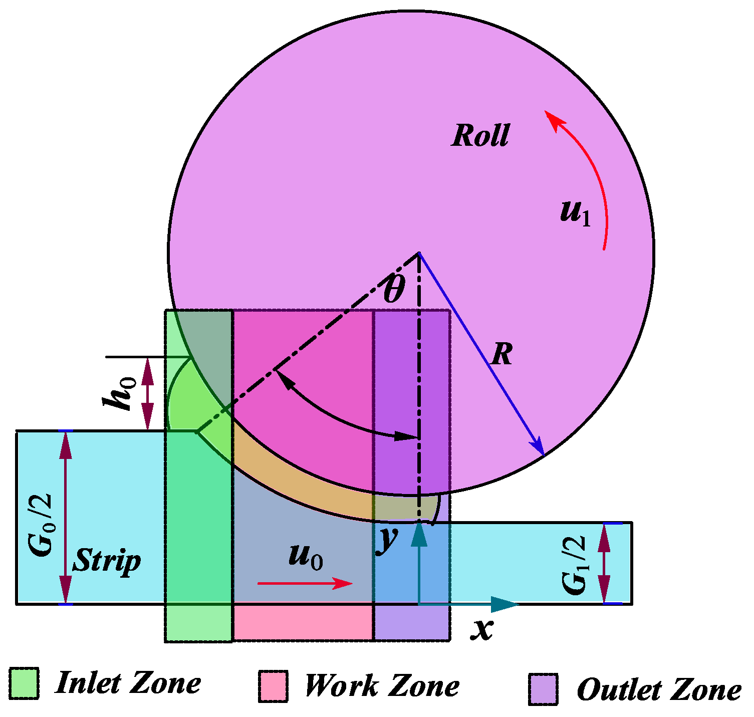
Figure 2 presents a schematic diagram of the rolling process. Based on the principles of volume conservation at the interface of the rolled material and the continuity equation in fluid mechanics, the velocity and thickness distribution of the workpiece in the deformation zone can be obtained in Ref. [16].

$$u_x=u_a{G}_0/G$$

(12)

$$h_f=\left(u_a+u_1)/(u_x+u_1\right)h_e$$

(13)

$$G=G_0\left(1-\epsilon \right)+{\left(l-x\right)}^2/R$$

(14)

In the equation, $h_0$ represents the initial thickness at the entry, $u_a$ denotes the velocity at the entry of the workpiece, $u_x$ represents the velocity of the workpiece in the deformation zone, $\epsilon$ represents the reduction rate of the workpiece, $G_0$ represents the initial thickness of the workpiece, $G$ denotes the thickness of the workpiece during the rolling process, and $R$ represents the radius of the rolling roll. Additionally, $l$ represents the length of the contact between the workpiece and the roll.

$$l=\sqrt{R△h+{\left[8Rp\left(1-{\gamma }^2\right)/\pi E^{\prime }\right]}^2}+8Rp\left(1-{\gamma }^2\right)/\pi E^{\prime }$$

(15)

The dimensionless thickness of the oil film in the Reynolds equation is commonly referred to as the film thickness ratio, denoted as $H$ is:

$$H=hR/l^2$$

(16)

The dimensionless velocity of the workpiece, denoted as $U$ is:

$$U={\eta }_{0}u/E^{\prime }R$$

(17)

The dimensionless thickness of the workpiece, denoted as $\overline{G}$ is:

$$\overline{G}=GR/l^2$$

(18)

Accurate modeling and prediction of the film thickness is crucial for understanding the lubrication conditions and optimizing the performance and efficiency of the rolling process. Composition of the film thickness at the rolling interface is shown in Figure 3. The film thickness equation is as in Ref. [17]:

$$h\left(x\right)=h_0+h_f+h_R+\delta$$

(19)

$$\delta =x^2/2R$$

(20)

$$\delta =2{\int }_{x_a}^{x_b}P\left(x^{\prime }\right)ln\mid x-x^{\prime }\mid d{x}^{\prime }/\pi E$$

(21)

The film thickness composition of the rolling interface is shown in Figure 4, where $h_0$ represents the film thickness of the rigid body’s central oil film, $h_f$ denotes the oil film thickness generated by the reduction in the workpiece, $\delta$ represents the oil film thickness generated by the equivalent deformation of the workpiece and rolling roll under load, and $h_R$ represents the roughness amplitude, which is $R_q$ in this study. The zero point of the x-axis is located at the exit position.

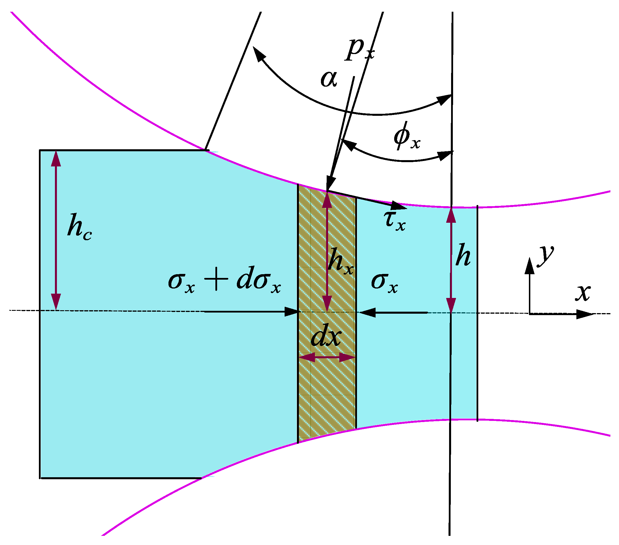
The total interface load at the lubricated contact interface is shared between the contact of rough asperities and the pressurized lubricant in the rough valleys. The load balance equation relates the total interface load $P$ to the roughness load $P_1$, the lubrication load $P_2$, and the contact area $U$ [17].

$$P=U{P}_1+\left(1-U\right)P_2$$

(22)

$$\left({\sigma }_x+d{\sigma }_x\right)\left(h_x+d{h}_x\right)-{\sigma }_x{h}_x+2pdx\cdot \mathit{tan}\varphi \mp 2{\tau }_{s}dx=0$$

(23)

The negative sign “$\mp$” indicates the direction from the entry position to the neutral point, while the positive sign indicates the direction from the neutral point to the exit position. At the neutral point, ${\tau }_s$ is equal to 0. Neglecting the second-order term $d{\sigma }_x\cdot d{h}_x$, and considering that during rolling, $\mathit{tan}\varphi =\frac{dh}{2dx}$ [18], the elemental force equation can be simplified as follows:

$$\left({\sigma }_x+p\right)\frac{d{h}_x}{dx}+h_x\frac{d{\sigma }_x}{dx}\mp 2{\tau }_s=0$$

(24)

The lubrication flow conditions at the rolling interface are described by the Reynolds equation:

$$\frac{\mathrm{d}}{\mathrm{d}\mathrm{x}}\left(\frac{\mathsf{\rho }{\mathrm{h}}^3}{\mathsf{\eta }}\frac{\mathrm{d}\mathrm{p}}{\mathrm{d}\mathrm{x}}\right)=12{\mathrm{u}}_{\mathrm{s}}\frac{\mathrm{d}\left(\mathsf{\rho }\mathrm{h}\right)}{\mathrm{d}\mathrm{x}}$$

(25)

Its dimensional equation is as follow:

$$\frac{\mathrm{d}}{\mathrm{d}\mathrm{X}}\left(\mathsf{\epsilon }\frac{\mathrm{d}\mathrm{P}}{\mathrm{d}\mathrm{X}}\right)-\frac{\mathrm{d}\left({\mathsf{\rho }}^{\mathrm{*}}\mathrm{H}\right)}{\mathrm{d}\mathrm{X}}=0$$

(26)

The boundary conditions for the Reynolds equation as follow:

Inlet point $P\left(X_0\right)=0$;

Outlet point $P\left(X_c\right)=0$, $\frac{dP\left(X_e\right)}{dX}=0$

During the line contact process at the rolling interface, the influence of temperature on the rolling process needs to be considered. In addition to the isothermal line contact elastohydrodynamic lubrication calculation, the energy equation is incorporated, and temperature conditions are set for the upper and lower surfaces of the rolling element [19,20].

$$c_p\rho \left(u\frac{\partial T}{\partial x}-w\frac{\partial T}{\partial z}\right)=k\frac{{\partial }^{2}T}{\partial z^2}-\frac{T}{\rho }\frac{\partial \rho }{\partial T}\left(u\frac{\partial p}{\partial x}\right)+\eta {\left(\frac{\partial u}{\partial z}\right)}^2$$

(27)

The temperature conditions for the upper and lower surfaces is as follows:

$$T\left(x,0\right)={\left.\frac{k}{\sqrt{\pi {\rho }_1{c}_1{k}_1{u}_1}}{\int }_{-\infty }^x\frac{\partial T}{\partial z}\right|}_{x,0}\frac{ds}{\sqrt{x-s}}+T_0$$

(28)

$$T\left(x,h\right)={\left.\frac{k}{\sqrt{\pi {\rho }_2{c}_2{k}_2{u}_2}}{\int }_{-\infty }^x\frac{\partial T}{\partial z}\right|}_{x,h}\frac{ds}{\sqrt{x-s}}+T_0$$

(29)

The coupling relationship between the viscosity, pressure, temperature, and density of the lubricant can be expressed using the Roelands equation [21].

$$\eta ={\eta }_0\mathit{exp}\left\{\left(\mathit{ln}{\eta }_0+9.67\right)\left[{\left(1+p/p_0\right)}^2{\left(\frac{T-138}{T_0-138}\right)}^{-1.1}-1\right]\right\}$$

(30)

$$\rho ={\rho }_0\left[1+\frac{0.6p}{1+1.7p}+D\left(T-T_0\right)\right]$$

(31)

The dimensional equations of the above equation is as follows:

$${\eta }^{*}=\mathit{exp}\left\{\left(\mathit{ln}{\eta }_0+9.67\right)\left[{\left(1+p_{H}P/p_0\right)}^z{\left(\frac{T-138}{T_0-138}\right)}^{-1.1}-1\right]\right\}$$

(32)

$${\rho }^{*}=1+\frac{0.6p}{1+1.7p}+D\left(T-T_0\right)$$

(33)

4. The Calculation Process

This paper aims to investigate the working characteristics of the rolling interface, including stress distribution, oil film pressure, and thickness distribution at the rolling interface. The lubricated friction contact at the rolling interface is a typical line contact, and the multigrid method is commonly used for solving the line contact problem. The multigrid method is developed for solving large algebraic equation systems using iterative methods. When solving the algebraic equation system with iterative equations, the discrepancy between the approximate solution and the exact solution can be decomposed into different frequency components. The high-frequency components are quickly eliminated on dense grids, while the low-frequency components can only be eliminated on sparse grids. By employing the multigrid method, iterations can be alternated between dense and sparse grids, enabling the rapid elimination of high-frequency and low-frequency components, and minimizing the computational effort required [22].

The iterative process includes pressure correction and rigid body displacement correction required for load adjustment, all performed within a specific grid. The rolling interface is often subjected to high pressure, making it challenging to solve the numerical calculations using the Gauss–Seidel iteration method due to the risk of divergence [23]. In this paper, we employ the Jacobi bipole iteration method. The pressure correction equation can be written as follows:

$$\overline{P_i}=\widetilde{P_i}+c_1{\delta }_i$$

(34)

In the equation, $c_1$ represents the relaxation factor, ${\delta }_i$ represents the pressure correction term, and $\overline{P_i}$ and $\widetilde{P_i}$ represent the pressure before and after the iteration correction, respectively.

Due to the variations in temperature in the energy equation, viscosity in the viscosity–pressure–temperature equation, and elastic deformation in the film thickness equation with respect to pressure, the computational procedure in this study follows the following steps: first, an initial pressure distribution (Hertz contact pressure) and temperature distribution (uniform temperature field) are specified. The film thickness and viscosity values are then calculated based on the given pressure distribution. Next, the Reynolds equation is employed to solve for the new pressure distribution, with iterative corrections applied to the previous pressure distribution. The energy equation is subsequently utilized to solve for the temperature, considering the newly corrected viscosity values. The pressure is iteratively solved again using the newly corrected temperature and viscosity values. This iterative process is repeated until the difference between the pressures obtained from two consecutive iterations becomes sufficiently small, indicating convergence. Finally, the final pressure distribution, film thickness with elastic deformation, and temperature distribution are determined. The above-mentioned computational procedure, which takes into account the variations of temperature, viscosity, and elastic deformation with respect to pressure, is significant for the field of mechanical engineering. The simulation parameters are shown in

Table 1. Numerical simulation parameters.

Name	Symbol	Value
Equivalent Elastic Modulus of the Rolled Material (GPa)	$E^{\prime }$	70
Initial Viscosity of the Lubricant (mPa·S)	${\eta }_0$	210
Hardness of the Rolled Material (HB)	$H$	132
Inlet Thickness (mm)	$G$	2.605
Reduction Ratio (%)	$\epsilon$	0.1, 0.2, 0.3, 0.6
Roll Radius (mm)	$R$	200
Initial Ambient Temperature (°C)	$T\left(\mathrm{0,0}\right)$	29.85
Initial Ambient Temperature (m/s)	$u_1$	3.6 m/s
Rolling Speed (m/s)	$u_2$	1.4, 2.2, 3.2, 5.8
Surface Profile Parameters	${\lambda }_s$	1
Surface Roughness (um)	$R_q$	0.6

, and the simulation process is shown in Figure 5.

5. Discussion

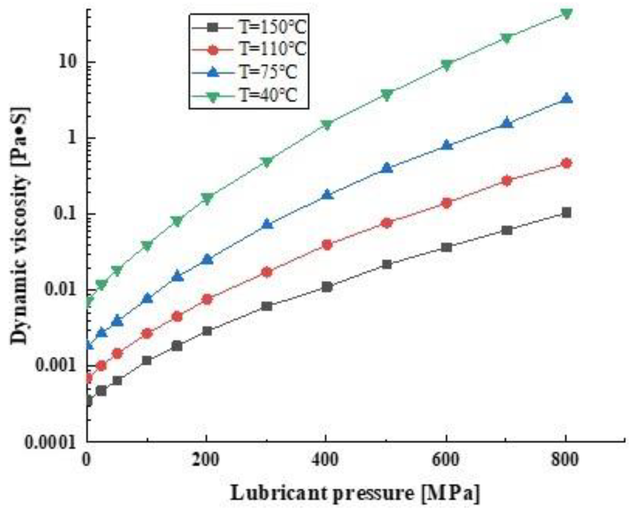
The dynamic viscosity curve of the lubricant is shown in Figure 6. It can be observed that the viscosity of the lubricant is significantly affected by pressure. As the pressure increases, the viscosity also increases. At lower pressures, the molecules of the lubricant are further apart, resulting in better flowability and lower viscosity. However, as the pressure increases, the intermolecular forces between the lubricant molecules become stronger, leading to a decrease in intermolecular distance and a reduction in flowability, resulting in an increase in viscosity. Moreover, it is evident that the viscosity of the lubricant decreases significantly with increasing temperature. As the temperature increases, the thermal energy of the lubricant molecules increases, weakening the intermolecular forces and enhancing the flowability of the lubricant, resulting in a decrease in viscosity.

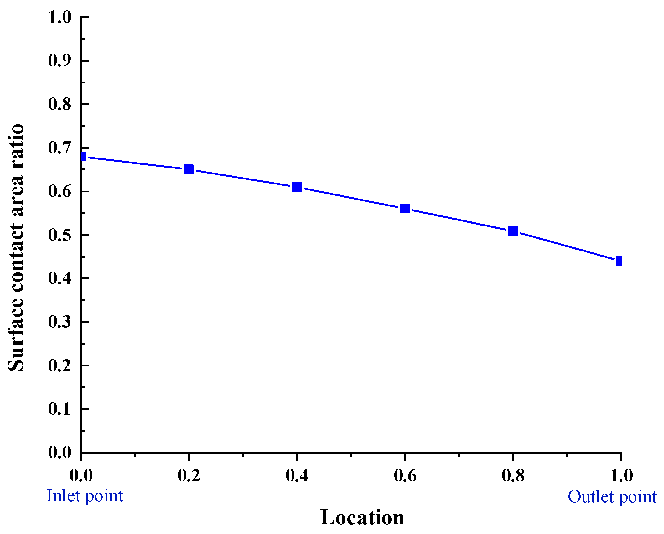
The change in contact area ratio along the rolling interface from the inlet to the outlet is illustrated in Figure 7. It can be observed that the contact area ratio gradually decreases in the outlet direction. This phenomenon can be attributed to two factors. Firstly, the rolling pressure initially increases and then decreases. The decrease in pressure mitigates the extent of plastic deformation of the roughness on the rolling interface. Secondly, the lateral metal plastic deformation intensifies near the outlet during the rolling process, resulting in a reduced contact probability of the contact area.

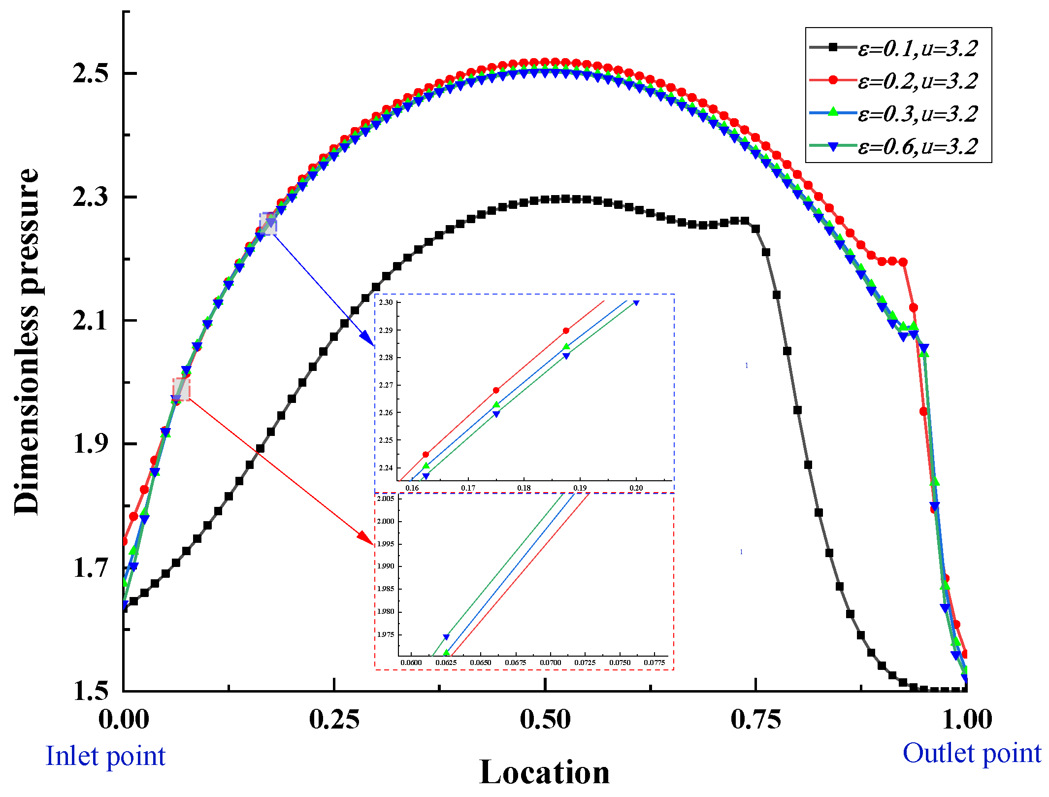
Figure 8 presents the distribution of oil film pressure at the lubricant interface under different rolling reductions when the rolling speed $u=3.2 \mathrm{m}/s$. The pressure distribution follows a typical linear contact elastohydrodynamic pressure distribution, with the pressure curve exhibiting a parabolic shape. Due to the roll entrainment effect, an oil film pressure is already formed at the rolling entrance. The oil film pressure at the exit does not follow a fixed pattern with the rolling reduction rate. At $\epsilon =0.2$, the maximum oil film pressure is observed at the entrance. Due to the sudden change in pressure at the exit, the oil flow rate increases, resulting in a secondary pressure peak before the exit. The maximum secondary pressure peak is observed at $\epsilon =0.2$. Based on the graph, it can be inferred that the oil film pressure is relatively low at smaller rolling reduction rates ($\epsilon =0.1$). As the reduction rate increases, the oil film pressure initially increases and then decreases. In the pre-rolling slip region, the oil film pressure at a reduction rate of 0.2 is slightly higher than that at 0.3 and 0.6. In the post-rolling slip region, there is not a significant difference in the oil film pressure between the reduction rates of 0.2, 0.3, and 0.6. However, at a reduction rate of 0.1, the oil film pressure notably decreases. The oil film pressure does not significantly increase with the increase in reduction rate. This is because at higher reduction rates, the temperature of the rolled material has a greater influence on the viscosity and pressure of the lubricant than the reduction rate itself.

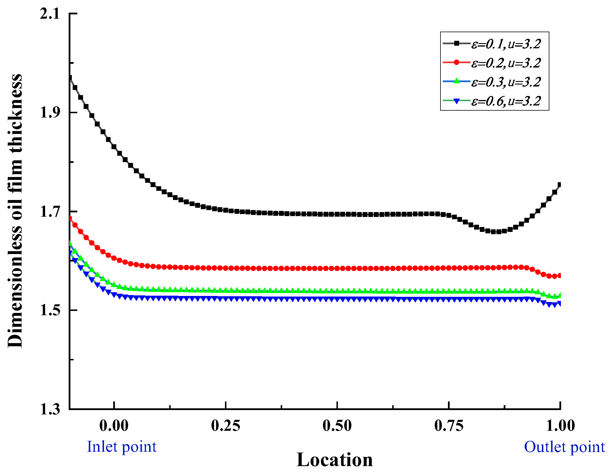
Figure 9 shows the distribution of oil film thickness at the rolling interface under different rolling reduction rates when the rolling speed $u=3.2 \mathrm{m}/\mathrm{s}$. The oil film thickness exhibits a wedge shape in the rolling region, with a slightly larger thickness at the entrance than at the exit. Consistent with the conclusion of oil film pressure, due to the roll entrainment effect, a certain pressure oil film thickness is already formed before the entrance. The oil film thickness sharply decreases at the entrance point, and there is a “necking” phenomenon at the exit region, where the oil film thickness increases. As the reduction rate increases, the oil film thickness gradually decreases. At a reduction rate of $\epsilon =0.1$, the dimensionless oil film thickness is approximately 1.7, while at $\epsilon =0.6$, the dimensionless oil film thickness is approximately 1.5. With the increase in reduction rate, the position of the “necking” phenomenon also gradually moves toward the exit region, and the decrease in oil film thickness at the “necking” point becomes less significant.

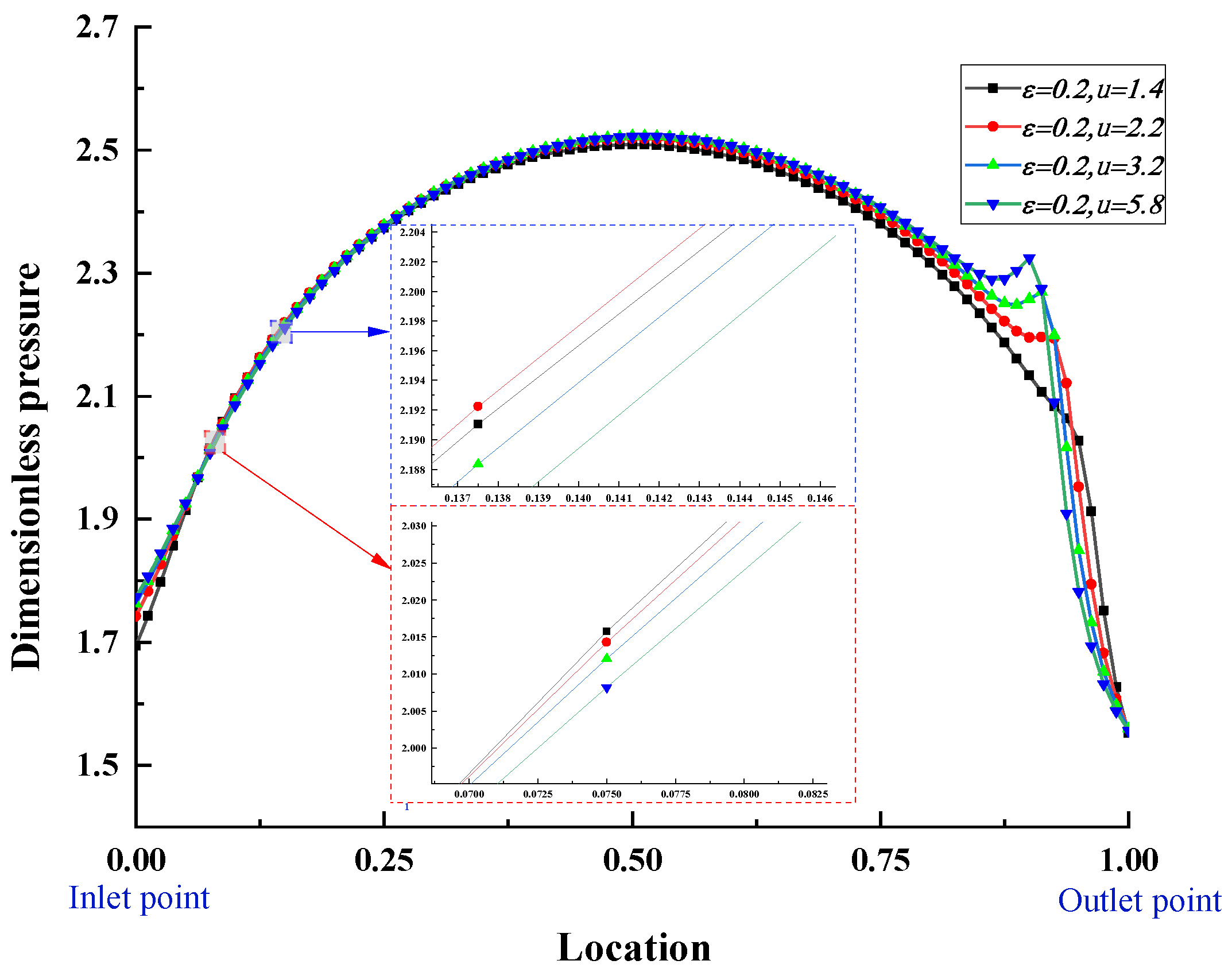
Figure 10 shows the distribution of the oil film pressure at the lubricant interface under different rolling speeds when the reduction rate is $\epsilon =0.2$. The influence of the rolling speed on oil film pressure is not significant, and the effect of the speed factor is mainly reflected in the exit region and the secondary pressure peak. When the rolling speed is higher, the value of the secondary pressure peak is also larger, but the difference between high- and low-speed rolling is less than 8%. The pressure at the exit region sharply drops to zero, especially at high rolling speeds, which may cause lubricant cavitation and lead to pitting or exacerbation of fatigue damage to the rolls.

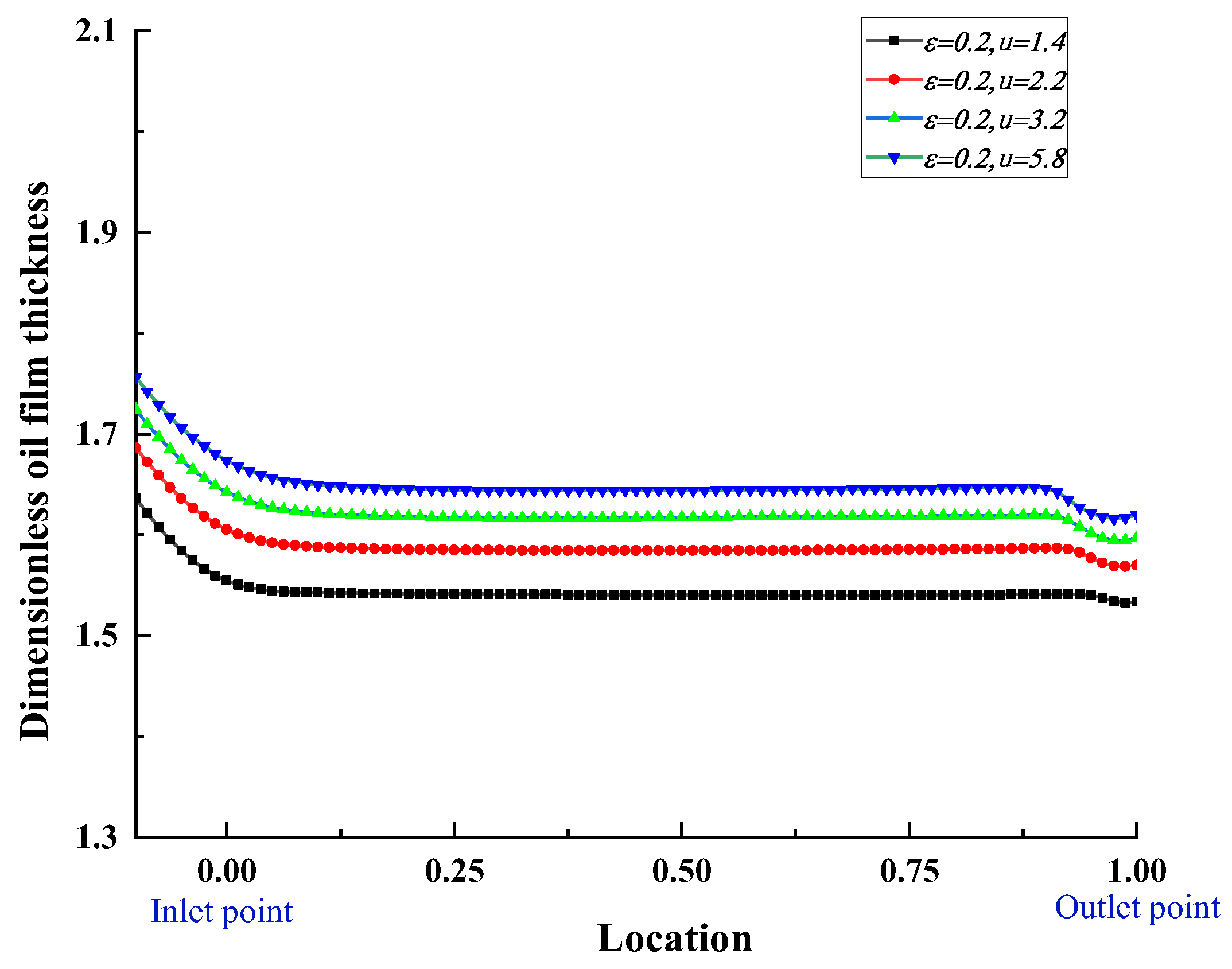
Figure 11 shows the distribution of interface pressure at the lubricant interface under different rolling speeds when the reduction rate is $\epsilon =0.2$. Unlike the small influence of rolling speed on oil film pressure, rolling speed has a significant effect on oil film thickness. As the rolling speed increases, the oil film thickness increases. At $u=1.4 \mathrm{m}/\mathrm{s}$, the dimensionless oil film thickness is approximately 1.54, while at $=5.8 \mathrm{m}/s$, the oil film thickness increases to 1.68. This is because as the speed increases, the viscosity of the lubricant also increases. Viscosity is a measure of the fluidity of the lubricant, and it describes the resistance of the lubricant to flow. When the speed increases, the increased viscosity of the lubricant leads to the formation of a thicker layer of oil film on the contacting surfaces. The increase in oil film thickness helps reduce the pressure of the surface contact, reducing the degree of friction and wear, but it may lead to a roll slip.

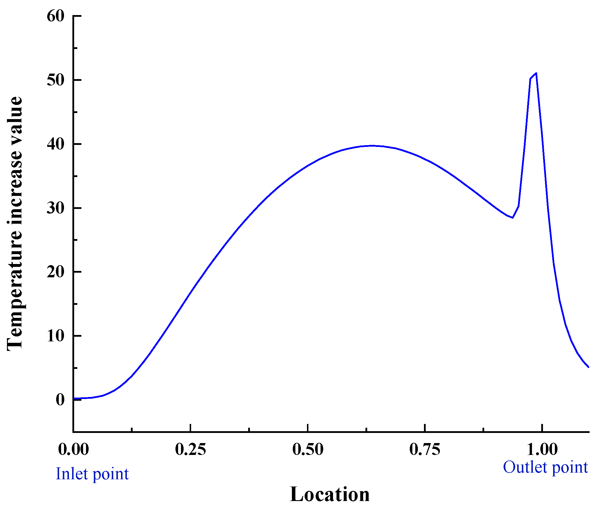
Figure 12 shows the distribution of the temperature increase during the rolling process with $\epsilon =0.2$ and $u=1.4 \mathrm{m}/\mathrm{s}$ The average temperature rise in the rolled piece is 26.7 K. There are two peak values in the temperature rise. The first peak appears near the neutral point and is relatively gentle. The second peak appears near the exit region, which is also the position of the secondary pressure peak. The gradient of the peak here is large, reaching 53 K.

Figure 13 shows the distribution of the interface stress during rolling considering the coupling effect of temperature field and fluid field. It is compared with Fu’s model [16], and the results show that the rolling interface model considering the coupling effect of the temperature field and fluid field has a consistent trend with Fu’s model, but there are differences in the amplitude and peak value of the rolling force. The peak value of the rolling force in the model considering the coupling effect of the temperature field and fluid field is lower than that of Fu’s calculation model, with a dimensionless value decreasing from 1.3 to around 1.15. The peak position also moves toward the exit, from 0.55 to around 0.7, and the pressure value at the exit is higher than that of Fu’s model. The comparison shows that the influence of temperature will reduce the stress peak of the rolled piece, and the overall stress of the rolled piece will also decrease.

6. Conclusions

• The pressure distribution of the interface lubricating oil follows a typical linear contact hydrodynamic pressure distribution, with a parabolic pressure curve. The oil film pressure does not significantly increase with the increasing pressure rate. This is because at higher reduction rates, the influence of the rolled piece temperature on the viscosity and pressure of the lubricant is greater than the influence of the reduction rate on the viscosity and pressure. A secondary pressure peak appears before the exit, and the secondary pressure peak is largest when ε = 0.2.
• The influence of the rolling speed on the oil film pressure is not significant, and its impact is mainly reflected in the exit area and the secondary pressure peak. When the rolling speed is higher, the numerical value of the secondary pressure peak is also larger, but the difference in low rolling speed is less than 8%. In contrast to the small influence of the rolling speed on the oil film pressure, the rolling speed has a significant impact on the oil film thickness. As the rolling speed increases, the oil film thickness increases.
• During the rolling process, the temperature of the rolled piece exhibits two peaks. The first peak occurs near the neutral point and is relatively gradual. The second peak occurs near the exit region, which is also the location of the secondary pressure peak. At this location, the peak gradient is significant, reaching 53 K. The influence of temperature will reduce the stress peak of the rolled piece, leading to a decrease in the overall stress of the rolled piece.