Abstract
The economy and rationality of the typical structural scheme for asphalt pavement are directly related to the formation of its service target. Based on the original highway asphalt pavement structure in Jilin Province, the evaluation index system was established by the research of the literature, investigation and Delphi method, and the results of expert consultation were tested by indicators such as enthusiasm, authority and coordination. The Kendall coordination coefficient was 0.803, indicating a strong degree of evaluation consistency. Then, using the finite element method and pavement economic analysis method, the key parameters of pavement structure asphalt, pavement design performance and economy are calculated. Finally, the key indicators in the pavement design process are quantified by using analytic hierarchy process (AHP) and gray relational theory, the weight of each key indicator and the correlation degree of the pavement structure are calculated, and pavement structure 1 is determined to be the best solution. The results show that a decision model for typical structural types of asphalt pavement can be established by using an improved gray relational analytic hierarchy process. In this study, the decision-making model can quickly and conveniently determine the most suitable typical pavement structure, the selected structures are checked, and the calculation results meet the requirements of the specification. However, given the limited reference cases, the proposed pavement structure decision-making method needs to be verified and improved through more practical applications.
1. Introduction
In the decision-making process of traditional pavement structures, the method of comparing pavement performance indicators is usually used to determine the appropriate pavement structure, but this evaluation method is relatively single and incomplete. As we all know, in addition to the road service performance index, economic rationality is another important determinant for comparing and selecting various design schemes. Therefore, in the field of road design, technical evaluation and economic evaluation of the design scheme are inseparable when designers are faced with deciding upon the type of pavement structure. However, there are few research methods and models using comprehensive design indicators for analysis, and many studies on pavement structures still rely on a single indicator, such as the thickness of the asphalt layer structure and mechanical indicators. This design method is obviously not comprehensive [1,2,3]. There is a certain correlation between the economy and the life of the pavement, for example, low initial cost, high post-maintenance cost, high initial cost, long pavement service life and low post-maintenance cost [4,5]. In addition, the quantity of high-quality asphalt produced in China is limited, imported asphalt is expensive, and the pavement structure and cost of asphalt pavement are closely related. In this case, it is necessary to select a combination type of pavement structure with different asphalt layer thicknesses according to technical and economic analyses. In the design and decision-making related to high-grade highway pavement, comprehensively considering various factors and selecting a reasonable type of pavement structure is a problem to be solved.
To seek a pavement structure with long life while taking into account cost, many scholars have conducted in-depth research in recent years. In terms of key indicators of pavement performance, various factors have been studied: Pan et al. [6] proposed that rutting is the most severe pavement deterioration of expressways. Fardin [7] proposed that fatigue cracking is more damaging than rutting on the roller-compacted concrete-base composite pavement. Li et al. [8] proposed that cracking in asphalt concrete layers is among the driving modes of flexible pavement deterioration. Cho et al. [9] proposed that delamination or debonding problems are particularly more severe for asphalt pavements that are subjected to heavy vehicle loads, especially horizontal surface shear forces that are due to braking and turning of vehicle tires. Yang et al. [10] proposed that shear fatigue damage is one of the main asphalt pavement failure modes. Interlayer fatigue resistance is also an important property in ensuring the durability and stability of asphalt pavements. In terms of economic performance indicators, additional work has been performed: Chong et al. [11] concluded that pavements without the need for reconstruction in the analysis period are generally more economical and environmentally friendly than those having to be reconstructed. However, designs that are too conservative lead to higher costs, greater energy consumption and greenhouse-gas emissions. Han et al. [12] established a decision model that fully considers the comprehensive maintenance benefit–cost ratio during the whole life cycle of the road. To overcome problems of experience-led manual decision-making, the decision-making between pavement conditions and maintenance plans was based on a data mining technique. Shon et al. [13] presented a pavement management framework that involves multiscale decisions, including system-level budget allocations, group-level inspections and facility-level maintenance, rehabilitation and reconstruction strategies. Considerable data analyses [14,15,16] reveal many cases of being focused on choosing typical pavement structures, but there are very few studies that take into account both work performance and economic performance and involve quantitative analysis.
Analytic Hierarchy Process (AHP) is a decision analysis method combining qualitative and quantitative approaches to solve complex multi-objective problems. Gray theory proposes the generalization of gray correlation analysis for each subsystem and intends to seek the numerical relationship between each subsystem (or factor) in the system through a certain method. The analytic hierarchy process and gray relational theory have been widely used in the field of pavement design. Han et al. [17] presented a decision-making method for asphalt pavement maintenance using an improved weight random forest algorithm based on correlation analysis and the AHP. Esmaeeli et al. [18] used the fuzzy real options methodology to help highway management organizations select the optimum alternative for project implementation. Yu et al. [19] presented and demonstrated a methodology for evaluating a microsurfacing treatment of asphalt pavement based on the gray system model and gray relational degree theory. Wang et al. [20] combined the results of gray relational analysis and the gray prediction methodology to establish gray-model-based smoothness predictions by using influencing factors similar to those used in the Mechanistic-Empirical Pavement Design Guide. However, the combination of the AHP and gray theory is rarely applied in the field of typical pavement structure decision-making. The judgment matrix in the AHP is completely determined by expert experience, and it is difficult to exclude the influence of subjective factors on the index weight. The gray correlation method is calculated based on the real data of the scheme, and the calculation results are relatively objective. When the traditional AHP calculates the comprehensive weight, it is only a simple synthesis of the index results and does not organically integrate the two methods to obtain the weight. To comprehensively consider these factors and choose a reasonable type of pavement, the new AHP combined with gray relational theory is a good way to solve this problem. At the same time, in the analysis of various factors of road construction investment decisions, the pavement performance index and economic evaluation index can be quantified, but the judgment matrix can only be used for qualitative analysis. Therefore, after the improvement of gray relational theory, the AHP is a new method to effectively address those complex problems that cannot be fully analyzed by using quantitative methods. It is a decision-making method combining quantitative and qualitative analyses. The characteristics of AHP, gray relational theory and improved AHP are summarized in Table 1.

Table 1.
Comparison of this study with existing research methods.
In summary, to improve the performance of pavement and reduce the cost of road construction and maintenance, we propose an improved AHP decision-making method to determine the optimal pavement structure.
2. Typical Pavement Structure Decision Process
Design evaluation can accurately reflect the quality of engineering projects. Through reasonable design evaluation methods, quantitative analysis of various indicators of highway construction can be conducted to effectively compare schemes and improve the quality and economic benefits of pavement engineering. The typical structure evaluation process for asphalt pavement in this study is as follows. First, the evaluation index layer and criterion layer of a typical pavement structure are constructed through literature and project historical data reviews. Then, according to the expert’s suggestion, the hierarchical structure model of the index system is constructed, and the comprehensive weight of each index is calculated based on the AHP. Next, the finite element (FE) model is used to build the model and calculate the performance and economic indicators. Finally, the gray relational degree is calculated for multiple indicators through the gray relational analysis method, and the one with the highest relational degree is the optimal solution. Figure 1 shows the evaluation process for the typical structure of the optimal pavement.
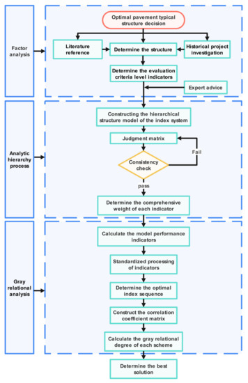
Figure 1.
Optimal pavement structure evaluation process.
3. Establishment of Evaluation System for Typical Pavement Structure
3.1. Optimal Decision-Making Process for Typical Pavement Structure
Because there is no clear and easy-to-use decision-making method for pavement structure, the pavement structure scheme of expressways in Jilin Province is not unified. Therefore, this study selects four commonly used highway pavement structure schemes in Jilin Province. The four schemes taken in this study are all of this structure, and the structure is shown in Figure 2.
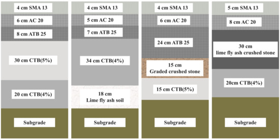
Figure 2.
Four typical pavement structure schemes.
3.2. Determination of the Evaluation Indicators
Pavement performance provides a basis for the comparison of the selection of pavement design schemes, but it is not the only reason for deciding on the choice of pavement type. The selection of typical pavement structures should also account for factors such as initial investment and total investment in the whole life cycle. A reasonable pavement design scheme should unify technical rationality and economic rationality.
3.2.1. Technical Indicators
From the perspective of technical rationality, there are multiple factors that need to be considered when selecting the type of pavement, mainly fatigue performance, antirutting performance and lateral deformation performance, such as rutting and sliding damage in high-temperature areas and fatigue cracking in low-temperature and heavy-traffic areas.
Therefore, according to the above performance requirements, six pavement performance parameters are proposed: stress and strain at the bottom of the asphalt layer, permanent deformation of the asphalt layer, the compressive strain on the top surface of the subgrade and horizontal shear stress and strain of the pavement.
3.2.2. Economic Indicators
From the perspective of economic rationality, the economic evaluation of the design scheme is an important basis for the comparison and selection of pavement structures. However, because of the various asphalt pavement structure schemes, the building materials and construction methods used are also different, but for a high-grade highway to be built, they play the same role or yield the same benefits. For the four schemes with the same benefits but different input costs, the present value method of total life cycle cost is most suitable when evaluating their economic advantages and disadvantages. The present value method of the total life cycle cost entails comparing the expenses invested by each program at different times, according to the social discount rate stipulated by the state, to the present value. The scheme with a low present value has an economic advantage. When choosing the type of pavement, the main factors considered are the initial investment and the present value of the total cost of the whole life cycle.
3.3. Factor Analysis
The relative importance of the indicators in the criterion layer and the target layer is scored by searching the literature and research by road design departments and discussing and communicating with relevant road experts.
3.3.1. Expert Scoring System
Two rounds of expert correspondence were conducted in this study, and the first questionnaire was established based on the initially constructed index system. Experts assigned evaluation indices according to their importance, familiarity, judgment basis and academic level. The expert scoring criteria are summarized in Table 2.
Table 2.
Expert scoring criteria.
In order to ensure the validity of the results of this study, the research team reviewed a large number of studies and comprehensively screened the evaluation indicators in combination with expert opinions. The analysis results of the first round of surveys are shown in Table 3. The average score of the Antifreeze performance of the pavement indicator is less than 70 points, and the coefficient of variation is greater than 0.25; therefore, the indicator is canceled. Table 4 shows the results of the second round of expert consultation, and all indicators meet the screening requirements.
Table 3.
Results of the first round of expert consultation.
Table 4.
Results of the second round of expert consultation.
3.3.2. Consistency Evaluation of Expert Consultation Results
- (1)
- The degree of positivity
The degree of positivity is usually determined by the positivity coefficient, which is equal to the number of questionnaires returned divided by the number of questionnaires published. The positive coefficient of the two rounds is 100%.
- (2)
- Degree of authority
The degree of authority usually depends on the judgment basis of experts, the familiarity with indicators and the academic level. Table 4 lists the scoring criteria for the importance of indicators, professional familiarity and academic level. Authority coefficient = (judgment coefficient + familiarity coefficient + academic level)/3. The authoritative coefficient of this study is 0.918.
- (3)
- Degree of coordination
Using the Kendall coordination coefficient to test the consistency of the research evaluation, it can be seen from Table 5 that the Kendall coordination coefficient test of the two survey results showed significance (p = 0.000 < 0.05), which means that the evaluations of the 20 experts are related. In addition, the coefficient of variation of the evaluation results of all indicators is less than 0.09, indicating that the coordination of experts in the two rounds is good. Judging from the results of the second expert consultation after index optimization, the Kendall coordination coefficient is 0.803, which is greater than 0.8, indicating a strong degree of evaluation consistency.
Table 5.
Kendall coordination coefficient analysis results.
We use the AHP to calculate the importance weight value of the criterion layer to the target layer and the importance weight value of the index layer to the criterion layer. Based on the above principles and indicators, an evaluation index system for typical optimal pavement structure is established, as shown in Figure 3.
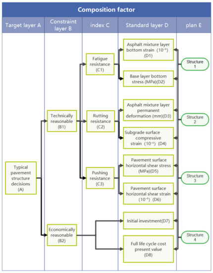
Figure 3.
Evaluation index system for typical optimal pavement structure.
3.4. Analytic Hierarchy Process
Before calculating the weights, it is necessary to perform a consistency check on the matrix in advance. First, the matrix needs to be normalized, then the maximum eigenvalue max is calculated, and the consistency index C.I. is calculated according to the maximum eigenvalue and the judgment matrix order n. Finally, the average random consistency index R.I. is introduced, and the test coefficient C.R. is calculated. When C.R. < 0.10, the test is passed; otherwise, it is not passed, in which case the comprehensive judgment matrix is adjusted according to the empirical method. The average random consistency index values are listed in Table 6. These were calculated as follows:
Table 6.
Average random consistency index values.
After checking the matrix consistency with Formulas (1)–(3), the comprehensive weight of the subindicators to the total target layer is finally established. This is calculated as W = (w1, w2, …, wn), where ≥ 0 and .
3.5. Relevance Calculation
To screen for the optimal scheme, based on the complex pavement structure index and the fuzzy evaluation characteristics, we adopted the gray relational analysis method to calculate the degree of correlation between the design scheme and the ideal design scheme and judge the degree of closeness of the connection according to the correlation coefficient.
If the decision-making system of the pavement structure design scheme consists of m schemes and n indicators, in this study, there are 4 schemes and 8 indicators, then the n index values of the I schemes can form a set Xi = (xi1, xi2, …, xin) (i = 1, 2, …, m), according to the n original index values of m schemes, and the following original scheme index matrix can be formed:
3.5.1. Normalization of Index Values
To eliminate the influence of dimension, the extremum method is used to normalize matrix X. In this study, the smaller the value of the evaluation index, the better the pavement structure scheme, and the quantitative index can be calculated according to
The normalized matrix is given by
3.5.2. Determine the Optimal Solution Index Set
The smaller the value of the evaluation index is, the better. Therefore, the optimal value is x0j = min(x1j, x2j, …, xmj); then the optimal index value is extremized to obtain the optimal value set X′0 = (x′01, x′02, …, x′0n).
3.5.3. Construction of the Correlation Coefficient Matrix
The following formula can be used to solve for the correlation coefficient between the original solution and the optimal solution:
where ρ ∈ [0, 1] is the resolution coefficient.
In summary, the correlation coefficient matrix can be obtained by using
3.5.4. Determination of Weighted Gray Relevance Degree
Ri (i = 1, 2, …, m) is the correlation degree of Xi to X0. According to the row vector Ei of the correlation coefficient and the weight vector W of each subindicator, the correlation degrees of each scheme can be obtained by using
The correlation degree Ri reflects the closeness of the relationship between Xi and X0 and the correlation between a single scheme and the best scheme. Therefore, the pros and cons of each scheme can be sorted according to the correlation degree.
4. Results and Discussion
4.1. Weight Ranking of Typical Pavement Structure Evaluation Index Based on the AHP
According to Table 7 and Table 8, the order of importance of key indicators for pavement structure decision-making is as follows: D3 > D1 > D2 > D8 > D4 > D7 > D5 = D6. In the traditional AHP, the order of the weights occupied by the four schemes is structure 1 > structure 4 > structure 2 > structure 3.
Table 7.
Evaluation index weight.
Table 8.
The traditional AHP method calculates the weight results.
4.2. Calculation of Relevance Degree of Typical Pavement Structure Based on the Gray Relational Method
4.2.1. Calculation of the Technical Performance Index of Pavement
We used the FE software Abaqus 6.14-4 for numerical simulation calculation. The FE analysis was performed for the four given typical asphalt pavement structures. The key parameters of pavement fatigue performance, rutting performance and pushing resistance were calculated.
Loads and Forms of Action
The pavement model uses a 100-kN single-axis double wheel as the design axle load, accounting for the horizontal load generated by braking. According to the relevant research results, the friction coefficient of the asphalt pavement was taken as 0.4, and the calculated axle load parameters were determined according to Table 9.
Table 9.
Design axle load parameters.
Pavement Geometry Model and Boundary Conditions
Figure 4 shows the pavement structure used for the FE calculation. The dimensions of the three-dimensional model were 6 m × 6 m × 3 m. Four typical structures commonly used for expressways in Jilin Province were selected. Table 10 summarizes the layer thicknesses and material properties of the simulated pavement structure. The modulus and Poisson’s ratio of each layer material in the pavement structure use the values recommended by the Asphalt Pavement Design Specification [21].
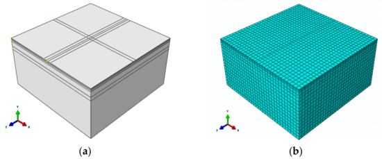
Figure 4.
Asphalt pavement structure model (a) and grid division diagram (b).
Table 10.
Pavement structure layer thickness and material composition.
To facilitate the calculation, the FE model has four constraints: There is no constraint on the surface of the model, there is no displacement on the two surfaces along the X-axis and Z-axis directions, and the bottom surface of the model has no displacement along the Y-axis direction. The asphalt material and soil in the pavement structure are nonlinear materials. The viscoelastic material of the asphalt pavement is calculated by using the Prony series [22]. The parameters of the Prony model are listed in Table 11. The elastic–plastic material of the subgrade soil is calculated by using the Drucker–Prager model. According to the Test Methods of Soils for Highway Engineering JTG E40-2007 [23], the cohesion and internal friction angle of the subgrade soil were measured through triaxial experiments. The parameters of the Drucker–Prager model are listed in Table 10.
Table 11.
Prony model parameters.
Pavement Performance Index Calculation Results
In addition to the permanent deformation index of the asphalt pavement, the calculation results of the FE model are summarized in Table 12.
Table 12.
Calculation results using FE pavement performance indicators.
Similarly, a permanent deformation prediction model [24] for the hot mix asphalt (HMA) layer can be expressed as
where hi is the midpoint depth of each layer, pi is the layered top compressive stress, R0i is the rut test permanent deformation, kri is the correction factor, ha is the asphalt mixture layer thickness (in mm), Tpef is the asphalt mixture layer equivalent temperature (in °C), Pi is the vertical compressive stress (in MPa) of the top surface of the ith layer of the asphalt mixture, which is calculated by using BISAR3.0 software, h0 is the rut test piece thickness (in mm) and Ne3 represents the equivalent design axle load cumulative design action times on the design lane within the design life. According to the prediction of the Jilin Provincial Highway Survey and Design Institute, Ne3 is 103,200,000 times. Table 13 lists the calculation results for the permanent deformation of the asphalt mixture layer.
Table 13.
Asphalt mixture layer permanent deformation.
Figure 5 shows that the tensile strain at the bottom of the asphalt layer of pavement structure 1 is the lowest, while the tensile stress of the base layer of structure 2 is the lowest. By considering the two indicators comprehensively, structure 2 is the best in terms of fatigue resistance of the pavement structure. The main reason for this is that a reasonable pavement structure will effectively reduce the fatigue strength of the asphalt mixture layer and the base and prolong the service life of the pavement structure. The asphalt layer of structure 1 is slightly thicker than that of structure 2, while the thickness of the base layer is thinner than that of structure 2, which will cause the stress of the pavement base to be slightly higher than that of structure 2. The tensile strain at the bottom of the asphalt layer and the tensile stress at the bottom of the base layer of structure 3 is the highest because a thicker asphalt layer is used, and a graded crushed stone flexible layer is set. The minimum thickness of the asphalt layer is structure 4, which leads to a high tensile stress of the subbase, and the pavement structure is very prone to fatigue damage. From the point of view of the fatigue resistance of the pavement structure, structures 2 and 1 are superior.
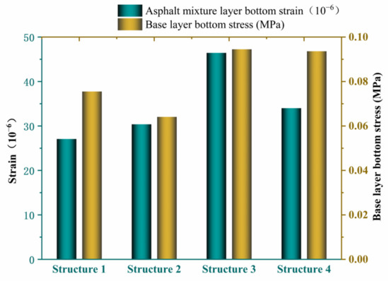
Figure 5.
Antifatigue performance parameters for pavement structure.
Figure 6 shows that the permanent deformation value of the asphalt layer of structure 3 is the highest, with the permanent deformation of structures 1 and 2 being somewhat less and the permanent deformation of pavement structure 4 being the least. The main reason for this difference is that the asphalt layer of structure 1 is the thickest, the thicknesses of the asphalt layer of structures 2 and structure 3 are basically the same, and the asphalt layer of structure 4 is the thinnest. This result is consistent with the previous study that indicated that the permanent deformation increases with the thickness of the asphalt layer [25]. In terms of the key parameters of the compressive strain on the top surface of the subgrade, structure 1 has the best performance, and the compressive strain on the top surface of the subgrade of structure 2 is the highest. Designers generally assume that smaller permanent deformations will reduce rutting damage in the pavement while also reducing costs. However, if the thickness of the asphalt layer is too thin, the pavement base is prone to fatigue cracking damage under repeated loads, which has a great impact on the service life of the pavement and subsequent maintenance. In addition, the low compressive strain on the top surface of the subgrade will effectively reduce the structural rutting of the asphalt pavement, which will improve the service life and service level of the pavement. Permanent deformation and vertical compressive strain on the top surface of the subgrade are the main factors affecting rutting. From the aspect of rutting performance, although the deformation performance of structure 4 is more prominent in the asphalt layer, the vertical compressive strain of the subgrade top surface is not ideal, and structure 1 has the most balanced performance.
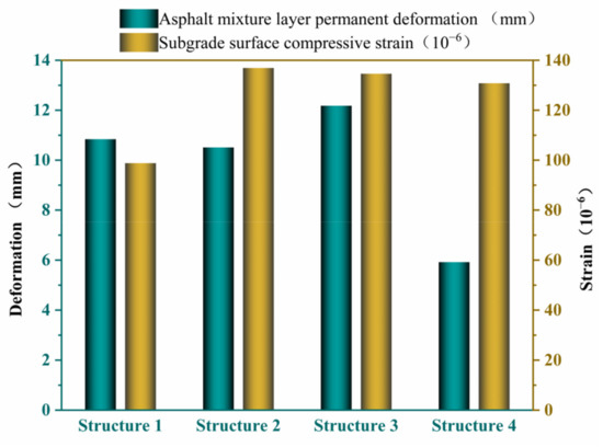
Figure 6.
Antirutting performance parameters for pavement structure.
Figure 7 shows that the horizontal shear stress and strain of structure 4 surface are the lowest, while that of structures 1, 2 and 3 are higher. The main reason for this difference is that the pavement of structure 4 is a double-layer asphalt structure, and the thickness of the asphalt layer is only 13 cm. After the asphalt layer and the base layer are bonded, the overall strength is improved, making it difficult to concentrate the horizontal shear stress of the road surface, and the overall stress and strain are low. However, the asphalt layer of the other structures is thicker, and the shear stress and strain of the road surface are higher. However, from the standpoint of antirutting performance of the pavement structure alone, structures 4 and 1 are better.
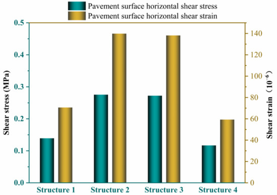
Figure 7.
Antipushing performance parameters for pavement structure (in driving direction).
In this study, many factors affecting pavement performance have been considered. In addition to the above-mentioned key parameters of pavement performance, the economic performance of the structural scheme should also be considered, and the optimal structural scheme should be finally determined.
4.2.2. Calculation of Economic Indicators
The expenses incurred at different times during the analysis period are converted into present value according to a predetermined discount rate, and by converting into a single present value, the pros and cons of the schemes in the whole life cycle can be compared on the basis of equivalent value. Because the case is focused on the same expressway and the same traffic volume was used, it was assumed that the annual average daily traffic volume (AADT) is 5000 vehicles/day and that the annual average traffic volume growth rate was 10%. For the convenience of analysis, a service life of 15 years was assumed, and the analysis period of each scheme was chosen to be the same. According to data from the United States, the actual cost of government investment is 4–5% [26], so the discount rate in this study was set as 4%.
According to relevant research [27,28], the following formula can be used to calculate the present value of expenses:
PWCx1,n is the present value of the total cost of scheme x1 in n years during the analysis period, which can be obtained by using the present value coefficient of the discount rate i in year t, which can be calculated by using
ICx1 is the initial construction cost of solution x1, RCx1,t is the reconstruction cost of solution x1 in year t, MCx1,t is the maintenance cost of solution x1 in year t, UCx1,t is the user fee of solution x1 in year t and SVx1,t is the residual value of the scheme x1 at the end of the analysis period.
The pavement residual value [29] at the end of the analysis period can be calculated according to
where the number of years from the construction year of the last LA remodel to the end of the life cycle, LB, is the expected service life of the reconstruction measure, and Cr is the construction cost of the reconstruction measure.
The reconstruction period can be calculated according to the pavement condition index (PCI). When PCI < 70, the original asphalt pavement needs to be reconstructed.
According to the literature [30], we can obtain the maintenance cost MCi and pavement condition index PCI. Substituting
gives the life factor β and shape factor α:
where h is the thickness of the pavement asphalt layer (in cm); ESAL is the daily equivalent axle load times (in times/day/lane); l0 is the initial deflection (0.01 mm); a, b, c and d are the regression coefficients or indices, the values of which can be selected according to Table 14 [27]; the standard axle load is 100 kN; and Kγα = 0.897 and Kγβ = 0.904 are the environmental impact coefficients in the Jilin area [31].
Table 14.
PCI decay equation regression parameter values.
Then, by using these life factors, PCI can be expressed as
Finally, the maintenance cost can be obtained as
The user fee consists of three items: fuel consumption, tire consumption and warranty material consumption. According to the literature [32,33], fuel consumption can be expressed by
wear cost of vehicle tires can be expressed by
and the material consumption cost can be expressed by
where IRI is flatness; a1, a2, b1 and b2 are regression coefficients; C0 and Cq are coefficients; Kp is the vehicle age index and Ckm is the average cumulative mileage (in km) for the vehicle. The regression coefficients are given in Table 15.
Table 15.
Parameters for calculating fuel consumption, wheel consumption and material consumption.
According to the types of vehicles in the Chinese Highway Asphalt Pavement Design Specification [24], the prices of fuels, tires and new cars in the market were investigated. These are summarized in Table 16.
Table 16.
Fuel, tire and new car prices.
The design width of the pavement was 15 m, the calculated length was assumed to be 1 km, and the calculated area of the pavement was 15,000 m2. According to the Jilin provincial engineering cost information network [34], the price of pavement structure materials was investigated. These values are summarized in Table 17. We used the following formula to calculate the initial investment C (in RMB) in pavement:
where A is the calculated area of the pavement (in m2), Pi is the unit price of each layer material (in RMB/m2), HG is the thickness of the graded crushed stone layer (in cm) and PG is the unit price of the graded crushed stone (in RMB/m2).
Table 17.
Pavement material prices.
As can be seen from Figure 8, the initial investment of structure 4 is the least, and the initial investment price of structure 3 is the highest. In the pavement structure, the asphalt concrete material is the most expensive, and the asphalt surface layer used in structure 4 is the thinnest, so the overall construction price is the lowest; the asphalt layer used in structure 3 is the thickest, so the initial investment is the highest. From the perspective of the whole life cycle, the present value of the cost of structure 1 is the lowest. According to the source of funds and the financing situation, by considering the feasibility of short-term investment, it is easy to choose a plan with low initial investment; from a long-term perspective, it is easy to choose a plan with a low present value of the total cost of the life cycle.
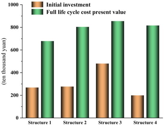
Figure 8.
Initial investment and present value of life-cycle cost for four pavement structures.
4.2.3. Calculation of Relevance Degree of Comprehensive Evaluation of Pavement Structure Based on Gray Relevance Theory
According to the performance calculation results for the four types of pavement schemes as the original index values, the matrix can be constructed in Table 18.
Table 18.
Initial matrix of key parameters of pavement structure.
The smaller the value of the above eight road performance indicators, the better, and an optimal value was set as the reference sequence [X0]. First, the original data were subjected to dimensionless processing according to Equation (5). The index normalization matrix is shown in Table 19.
Table 19.
Normalization matrix.
Figure 9 shows the correlation degree with different resolution coefficients. From the calculation results, when a = 0.5, the degree of discrimination becomes more obvious.
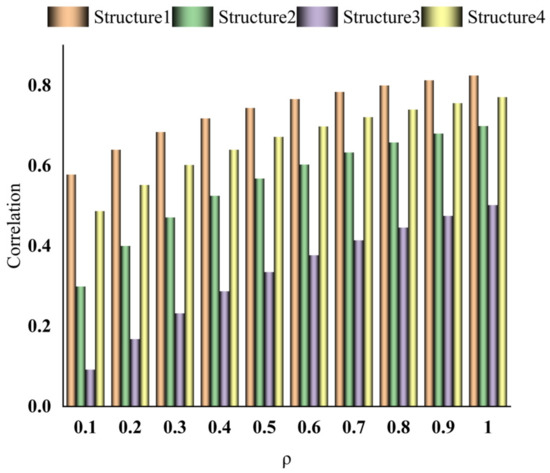
Figure 9.
Correlation at different resolution coefficients.
The correlation coefficient matrices are summarized in Table 20. The correlations of the four pavement structures are calculated according to Formula (10), and the final correlations are summarized in Table 21.
Table 20.
Correlation coefficient matrix.
Table 21.
Correlation of four typical structures calculated by the improved AHP method.
According to the results in Figure 10, R1 > R4 > R2 > R3. Therefore, pavement structure scheme 1 is the closest to the optimal scheme, and it is the best design scheme, and the difference between scheme 3 and the optimal design scheme is the greatest. Although the calculation results using the AHP method were roughly the same as those calculated by using the AHP and gray theory methods, the correlation between the traditional AHP structure 2 and structure 4 is very close and difficult to distinguish. The improved AHP combines the key parameters of the pavement structure, and the correlation degree becomes more obvious.
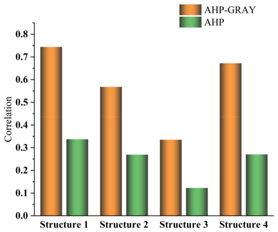
Figure 10.
Comparison of correlation results between AHP and improved AHP.
4.3. Optimal Selection Results and Discussion
Conducting research on the typical structure of expressways in Jilin Province is needed to improve the local road service level and provide cost savings for infrastructure construction. Finally, through the analysis and evaluation of the pavement structure in Jilin Province and via a comparison of the present value of the cost in the whole life cycle of the structure scheme, the improved AHP can effectively integrate the two most critical indicators involved in road construction and enable quantitative analysis of the calculation results through gray theory. This method of pavement structure decision-making, which integrates pavement performance and economics, can be applied in various regions of the world, facilitating the identification of the most cost-effective pavement structure scheme.
5. Failure Mechanism Analysis
5.1. Cement-Treated Material Base Layer
The fatigue cracking life prediction for the cement-treated layer can be calculated according to
Table 22 lists the parameters required to calculate the fatigue life model.
Table 22.
Fatigue life model parameters of cement-treated layer.
According to the design of the pavement structure, the fatigue cracking life (axial order) of the inorganic binder stable layer is greater than the design cumulative axis of 103,200,000 times (from the prediction of traffic based on the design report), meeting the specification design requirements.
5.2. HMA Layer Permanent Deformation
Table 23 lists the parameters required to calculate the permanent deformation of the asphalt layer.
Table 23.
Permanent deformation prediction model parameters for the HMA layer.
The permanent deformation of the HMA layer (in mm) can be calculated according to
where Rai is the permanent deformation of each layer (in mm) and [Ra] is the permissible permanent deformation in the design code (in mm).
According to the research in this study, the optimal pavement structure is obtained, and the permanent deformation of the HMA layer and the fatigue of the cement-treated layer can meet the specification requirements.
6. Conclusions
Decision-making for typical pavement structures based on life-cycle economic evaluation and key performance indicators using the AHP and gray relational theory have been investigated. The following conclusions can be made:
- (1)
- In this paper, the Delphi method and analytic hierarchy process are used to construct a decision-making index system for a typical pavement structure. The expert consultation was divided into two rounds. After the first round of the survey, we found that the average score of the antifreeze performance of the pavement index was low, and the coefficient of variation was greater than 0.25. The index was canceled, and the evaluation index system was optimized. After the second round of the survey, according to the survey data, the coordination coefficient increased by 24% compared with the first round, reaching 0.803, and the difference was statistically significant, ensuring the authority, reliability and consistency of the results.
- (2)
- Combined with the four typical structures used by the highway design department of Jilin Province, the finite element model was established by ABAQUS software, and the performance evaluation indexes required by the AHP were calculated. At the same time, according to the material price, design service life, traffic volume, initial cost of road construction and the present value of the whole life cycle cost, the economic evaluation indicators required by the AHP were calculated.
- (3)
- Using the improved gray relational AHP, an evaluation model of the asphalt pavement structure is established. The model organically combines the intermediate process of the two methods of the AHP and gray correlation, which reflects not only the objective situation but also the preference of human subjective factors for evaluation indicators. The evaluation results obtained in this way are more scientific and fairer.
- (4)
- The key technical indicators for the pavement are the permanent deformation of the asphalt layer and the tensile stress and strain at the bottom of the asphalt layer; the key economic indicator for the pavement is the present value of the full life cost. In decision-making for pavement structure, the key technical indicators of pavement performance are more important than the key economic indicator.
- (5)
- This study used the AHP-GRA method to make decisions on typical pavement structures in Jilin Province, and the results show that Pavement Structure 1 is an ideal choice for performance and economy. The fatigue cracking and permanent deformation of structure 1 are checked and calculated, which conforms to the requirements of the Chinese Asphalt Pavement Design Specification.
- (6)
- The improved AHP is used to comprehensively analyze the two key indicators, and the results show that structure 1 is the most suitable typical pavement structure for Jilin Province when the initial budget is relatively sufficient. However, if the initial budget is insufficient, then structure 4 can be considered.
Note that the conclusions obtained in this study are mainly applicable to the four typical structural schemes of the designated Jilin Province. However, when decisions about pavement structure are required in road construction, the analysis scheme presented in this paper can be used to determine a reasonable pavement structure.
Author Contributions
Data curation, M.Z.; Investigation, C.W.; Methodology, L.F.; Project administration, J.Y.; Writing—Original draft, M.Z.; Writing—Review & editing, J.Y. All authors have read and agreed to the published version of the manuscript.
Funding
This research was funded by [Jilin Provincial Department of Education Science and Technology Research Project] grant number [JJKH20220842KJ] and [Science and Technology Program of Shenzhen] grant number [JSGG20201103100601004]. The APC was funded by [Jilin Provincial Department of Education Science and Technology Research Project] grant number [JJKH20220842KJ].
Institutional Review Board Statement
Not applicable.
Informed Consent Statement
Not applicable.
Data Availability Statement
Not applicable.
Conflicts of Interest
The authors declare no conflict of interest.
References
- Hu, X.; Zhong, S.; Walubita, L.F. Three-dimensional modelling of multilayered asphalt concrete pavement structures: Strain responses and permanent deformation. Road Mater. Pavement Des. 2015, 16, 727–740. [Google Scholar] [CrossRef]
- Erlingsson, S. Rutting development in a flexible pavement structure. Road Mater. Pavement Des. 2012, 13, 218–234. [Google Scholar] [CrossRef]
- Wistuba, M.P.; Walther, A. Consideration of climate change in the mechanistic pavement design. Road Mater. Pavement Des. 2013, 14, 227–241. [Google Scholar] [CrossRef]
- Amini, A.A.; Mashayekhi, M.; Ziari, H.; Nobakht, S. Life cycle cost comparison of highways with perpetual and conventional pavements. Int. J. Pavement Eng. 2012, 13, 553–568. [Google Scholar] [CrossRef]
- Santos, J.; Ferreira, A. Life-cycle cost analysis system for pavement management at project level. Int. J. Pavement Eng. 2013, 14, 71–84. [Google Scholar] [CrossRef]
- Pan, Y.; Shang, Y.; Liu, G.; Xie, Y.; Zhang, C.; Zhao, Y. Cost-effectiveness evaluation of pavement maintenance treatments using multiple regression and life-cycle cost analysis. Constr. Build. Mater. 2021, 292, 123461. [Google Scholar] [CrossRef]
- Fardin, H.E.; dos Santos, A.G. Predicted responses of fatigue cracking and rutting on Roller Compacted Concrete base composite pavements. Constr. Build. Mater. 2021, 272, 121847. [Google Scholar] [CrossRef]
- Ozer, H.; Al-Qadi, I.L.; Singhvi, P.; Bausano, J.; Carvalho, R.; Li, X.; Gibson, N. Prediction of pavement fatigue cracking at an accelerated testing section using asphalt mixture performance tests. Int. J. Pavement Eng. 2018, 19, 264–278. [Google Scholar] [CrossRef]
- Cho, S.-H.; Karshenas, A.; Tayebali, A.A.; Guddati, M.N.; Kim, Y.R. A mechanistic approach to evaluate the potential of the debonding distress in asphalt pavements. Int. J. Pavement Eng. 2017, 18, 1098–1110. [Google Scholar] [CrossRef]
- Yang, K.; Li, R.; Yu, Y.; Pei, J.; Liu, T. Evaluation of interlayer stability in asphalt pavements based on shear fatigue property. Constr. Build. Mater. 2020, 258, 119628. [Google Scholar] [CrossRef]
- Chong, D.; Wang, Y.; Dai, Z.; Chen, X.; Wang, D.; Oeser, M. Multiobjective optimization of asphalt pavement design and maintenance decisions based on sustainability principles and mechanistic-empirical pavement analysis. Int. J. Sustain. Transp. 2018, 12, 461–472. [Google Scholar] [CrossRef]
- Han, C.; Ma, T.; Chen, S. Asphalt pavement maintenance plans intelligent decision model based on reinforcement learning algorithm. Constr. Build. Mater. 2021, 299, 124278. [Google Scholar] [CrossRef]
- Shon, H.; Lee, J. Integrating multi-scale inspection, maintenance, rehabilitation, and reconstruction decisions into system-level pavement management systems. Transp. Res. Part C Emerg. Technol. 2021, 131, 103328. [Google Scholar] [CrossRef]
- Geng, H.; Clopotel, C.S.; Bahia, H.U. Effects of high modulus asphalt binders on performance of typical asphalt pavement structures. Constr. Build. Mater. 2013, 44, 207–213. [Google Scholar] [CrossRef]
- Lv, S.; Yuan, J.; Peng, X.; Zhang, N.; Liu, H.; Luo, X. A structural design for semi-rigid base asphalt pavement based on modulus optimization. Constr. Build. Mater. 2021, 302, 124216. [Google Scholar] [CrossRef]
- Jiang, X.; Zeng, C.; Gao, X.; Liu, Z.; Qiu, Y. 3D FEM analysis of flexible base asphalt pavement structure under non-uniform tyre contact pressure. Int. J. Pavement Eng. 2017, 20, 999–1011. [Google Scholar] [CrossRef]
- Han, C.; Ma, T.; Xu, G.; Chen, S.; Huang, R. Intelligent decision model of road maintenance based on improved weight random forest algorithm. Int. J. Pavement Eng. 2022, 23, 985–997. [Google Scholar] [CrossRef]
- Esmaeeli, A.N.; Heravi, G. A decision support framework for economic evaluation of flexible strategies in pavement construction projects. Int. J. Pavement Eng. 2019, 20, 1342–1358. [Google Scholar] [CrossRef]
- Yu, J.; Zhang, X.; Xiong, C. A methodology for evaluating micro-surfacing treatment on asphalt pavement based on gray system models and gray rational degree theory. Constr. Build. Mater. 2017, 150, 214–226. [Google Scholar] [CrossRef]
- Wang, K.C.; Li, Q.; Hall, K.D.; Elliott, R.P. Experimentation with Gray Theory for Pavement Smoothness Prediction, Transportation Research Record. J. Transp. Res. Board 2007, 1990, 3–13. [Google Scholar] [CrossRef]
- JTG D50-2006; Specification for Design of Highway Asphalt Pavement. Ministry of Transport of the People’s Republic of China: Beijing, China, 2006.
- Park, S.W.; Schapery, R. Methods of interconversion between linear viscoelastic material functions. Part I—A numerical method based on Prony series. Int. J. Solids Struct. 1999, 36, 1653–1675. [Google Scholar] [CrossRef]
- JTG E40-2007; Test Methods of Soils for Highway Engineering. Ministry of Transport of the People’s Republic of China: Beijing, China, 2007.
- JTG D50-2017; Specification for Design of Highway Asphalt Pavement. Ministry of Transport of the People’s Republic of China: Beijing, China, 2017.
- Xu, Q.; Mohammad, L.N. Modeling Asphalt Pavement Rutting under Accelerated Testing. Road Mater. Pavement Des. 2008, 9, 665–687. [Google Scholar] [CrossRef]
- Ferreira, A.; Santos, J. Life-cycle cost analysis system for pavement management at project level: Sensitivity analysis to the discount rate. Int. J. Pavement Eng. 2013, 14, 655–673. [Google Scholar] [CrossRef]
- Li, N.; Huot, M.; Haas, R. Cost-Effectiveness-Based Priority Programming of Standardized Pavement Maintenance. Transp. Res. Rec. J. Transp. Res. Board 1997, 1592, 8–16. [Google Scholar] [CrossRef]
- Smith, K.L.; Titus-Glover, L.; Darter, M.I.; Von Quintus, H.; Stubstad, R.; Scofield, L. Cost–Benefit Analysis of Continuous Pavement Preservation Design Strategies versus Reconstruction, Transportation Research Record. J. Transp. Res. Board 2005, 1933, 83–93. [Google Scholar] [CrossRef]
- Al-Suleiman, T.I.; Shiyab, A.M. Prediction of Pavement Remaining Service Life Using Roughness Data—Case Study in Dubai. Int. J. Pavement Eng. 2003, 4, 121–129. [Google Scholar] [CrossRef]
- Sun, L. Structural Behavior Study for Asphalt Pavement, 1st ed.; China Communications Press: Beijing, China, 2005. [Google Scholar]
- JTG 003-86; Standard for Climatic Zoning of Highways. Ministry of Transport of the People’s Republic of China: Beijing, China, 1987.
- Watanatada, T.; Dhareshwar, A.M.; Lima, P.R. Vehicle Speeds and Operating Costs: Models for Road Planning and Management; International Bank for Reconstruction and Development: Washington, DC, USA, 1987. [Google Scholar]
- Dickey, J.W.; Miller, L.H. Road Project Appraisal for Developing Countries; National Academic: New York, NY, USA, 1984. [Google Scholar]
- Jilin Provincial Engineering Cost Information Network. Pavement Material Price. 2022. Available online: https://www.cczjxxw.com/dishi/sz/jgxx/scj.asp (accessed on 1 April 2022).
Publisher’s Note: MDPI stays neutral with regard to jurisdictional claims in published maps and institutional affiliations. |
© 2022 by the authors. Licensee MDPI, Basel, Switzerland. This article is an open access article distributed under the terms and conditions of the Creative Commons Attribution (CC BY) license (https://creativecommons.org/licenses/by/4.0/).