Abstract
The current analysis deals with radiative aspects of magnetohydrodynamic boundary layer flow with heat mass transfer features on electrically conductive Williamson nanofluid by a stretching surface. The impact of variable thickness and thermal conductivity characteristics in view of melting heat flow are examined. The mathematical formulation of Williamson nanofluid flow is based on boundary layer theory pioneered by Prandtl. The boundary layer nanofluid flow idea yields a constitutive flow laws of partial differential equations (PDEs) are made dimensionless and then reduce to ordinary nonlinear differential equations (ODEs) versus transformation technique. A built-in numerical algorithm bvp4c in Mathematica software is employed for nonlinear systems computation. Considerable features of dimensionless parameters are reviewed via graphical description. A comparison with another homotopic approach (HAM) as a limiting case and an excellent agreement perceived.
1. Introduction
Nanofluid is a kind of liquid that contains small-sized metallic particles having dimensions up to 1–100 nm. Usually, these small metallic particles are made up of graphite, carbon nanotubes, copper, aluminum, oxides, carbide nitrides, and many more. Choi [1] conducted an experimental examination that incorporating these nanoparticles in base liquids results in a significant upsurge in thermal conductivity and heat transfer behavior of base liquid. In recent times, many researchers, engineers, and scientists have utilized the concept of nanofluid to increase the thermal nature and heat transference rate of various base fluids for useful industrial and engineering processes. Buongiorno [2] proposes that this abnormal upsurge in thermal and heat transfer features, namely due to two main reasons, which are the Brownian movement and thermophoretic diffusion in base liquids. An extraordinary research has been undertaken to explore the heat transfer and the effects of thermal radiation by Daungthongsuk and Wongwises [3], Wang and Mujumdar [4,5], Kakac and Pramuanjaroenkij [6]. The results of magnetic field and nonlinear convective Williamson nanofluid in view of the radially stretchable surface with electrical application has been evaluated by Ibrahim and Gamachu [7]. The results of the activation energy of a mixed convective heat mass transfer effects of Williamson nanofluid, with heat generation and absorption over a stretching cylinder, were deliberated by Ibrahim and Negera [8,9]. Yusuf et al. [10] analyzed the influence of thermal radiation and entropy generation on a stretching sheet with chemical reaction in the presence of MHD flow of Williamson nanofluid. Aldabesh et al. [11] investigate the axisymmetric analysis for the Casson nanofluid due to parallel stretchable disks. Alhamaly et al. [12] have discussed thermal radiation effects on stagnation point nanofluid flow on a linearly stretching surface with heat transfer analysis. MHD and stagnation point nanofluid flow in view of the stretchable surface along with the variable thickness and radiation effects are evaluated by Ramesh et al. [13]. Several further investigators have indicated useful engineering applications of boundary fluid layer flow with thermal generation in view of stretching surfaces for different fields, such as polymer extraction, filing drawing, paper manufacturing, wire coatings analysis for glass fiber production and many more practical uses. Srinivasulu and Goud [14] have investigated heat mass flow and the impact of an aligned magnetic field on Williamson’s nanofluid over a stretching surface with convective boundary conditions. Effects of heat generation/absorption on magnetohydrodynamic, dissipative, and mixed convection boundary layer Cu-water nanofluid in a nonlinear stretching/shrinking sheet in the existence of heat generation/absorption and viscous dissipation is analyzed by Reddy et al. [15]. Nayak et al. [16] have diverted their attention toward the hydromagnetic three-dimensional convective flow of a nanofluid in view of the stretchable surface along with thermal radiation and variable magnetic field effect. Williamson fluid is a typical non-Newtonian fluid model having the shear thinning behavior. The model was proposed by Williamson [17]. Rasheed et al. [18] studied the hydromagnetic boundary layer flow of Jeffrey nanofluid past by vertically stretching a cylindrical sheet with Newtonian heating and dissipation effects. Later on, other researchers explored various features with different geometries and discussed flow, thermal and solutal fields by Ibrahim and Negera, [19], Vasudev et al. [20], Nadeem, and Hussain [21]. Gorla and Gireesha [22] have paid attention to stagnation point liquid flow and heat transfer characteristics of non-Newtonian Williamson nanofluid in view of stretching/shrinking sheet surface along with convective boundary conditions. The above-stated citations are all directly related to explored and boundary-layer flow of nanofluid along with the development of heat and thermal conductivity of base liquid over a stretching sheet with different geometrical aspects. The fluid flow and heat transfer of viscoelastic fluids in view of stretching sheet along with variable thickness non flatness can be more applicable to the situation in practical utilizations. Abbas et al. [23] examine entropy generation and heat transfer development on magneto-hydrodynamic slip flow of viscous fluid in a diverging tube. Fang et al. [24] investigated and found for the first time an analytical and numerical approach for the solution of two-dimensional boundary layer flow due to a non-flatness stretching sheet. Furthermore, the same problem was addressed by Subhashini et al. [25] by incorporating the energy term and observing the thermal boundary layer thicknesses for the first solution which were thinner than those of the second solution. A numerical and analytical investigation was carried out for the solution of viscoelastic non-Newtonian fluid over a stretching surface in the presence of porous medium as well as in the thermal radiation effects by Khader and Meghad [26]. Here some relevant applications based on citations of nanofluids directly related to the present investigation have been cited in [27,28,29,30,31].
2. Mathematical formulation
Here, we have assumed hydromantic two-dimensional Williamson nanofluid flow in view of a stretchable surface. The center is pointed out at a slit point from which the surface is drawn over the fluid medium. The sheet’s velocity, defined by the formula as here, lies in the direction of the stretchable sheet surface, the normal to stretching sheet. Further, we considered that the surface is not flat, and thickness is changing with the relation given by , positive constant such that the surface is thin enough, and is velocity power index. When , represent a flat sheet flow problem. An external magnetic field has been employed having strength in normal direction of fluid flow. As fluid has conducting behavior, the Reynolds number is less than one. The induced magnetic field effect is small in comparison to the applied field. Coordinates axes and flow model configuration is shown in Figure 1.
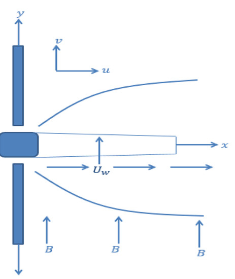
Figure 1.
Schematic flow and Coordinate system.
Cauchy stress tensor for Williamson fluid model defined by [19]:
Whereas denotes the extra stress tensor, represents the viscosity of the fluid as shear rate is zero and shows the viscosity for shear rate at infinite, where denotes time constant. denotes first Rivlin Erickson tensor, can be written by the relation given as below:
Herein, we have selected the case when and that of . Therefore may be written as mention below:
After utilizing the binomial series, we obtained as follow:
The mathematical expressions for two-dimensional flow laws are [21]:
Conditions are [21]:
where velocity components in x and y directions, is fluid density, is the gravity force, viscosity, kinematic viscosity, specific heat, is field strength, temperature, concentration, fluid temperature at wall, ambient temperature when . Herein Brownian diffusion-coefficient, thermophoretic diffusion-coefficient, ratio between effective heat capacity of nanoparticles material and heat capacity of the fluid, temperature dependent thermal conductivity by [32]:
Rosseland approximation for radiation defined by:
Here, denotes Stefan–Boltzmann-constant, is absorption coefficient. Further, we considered that temperature variations inside fluid, in such a way that factor can be written in the form of linear function of fluid temperature. We obtained series expression for by utilizing the Taylor theorem at stream temperature and ignoring higher powers of as:
By utilizing (7) and (8), we set:
By introducing similarity functions are:
Here, Equation (1) is true identically while (2)–(5) have the forms:
Following are the governing pertinent parameters appearing in (11)–(14) are defined as:
and elucidated magnetic field, Prandtl number, wall thickness parameter, radiation parameter, Lewis number, nanofluid heat capacity, Brownian diffusivity/thermophoretic diffusivity, Williamson fluid parameter and thermal conductivity parameter respectively.
Expressions of physical quantities are
Where are heat flux and mass flux:
By simplifying the above equations, we have
Here, is the local Reynolds number and
3. Numerical Scheme
In this section, the ordinary nonlinear coupled differential flow expressions (11)–(13), subject to conditions in (14) are addressed and solved numerically by utilizing computational algorithm bvp4c, a built-in function in Mathematica software. The nonlinear system of couple flow equations is changed to first order differential equations.
Let the appropriate transformation variables be defined by:
Transformed conditions are:
Asymptotic convergence is perceived to be achieved for . All computational outcomes achieved in this problem are subjected to error tolerance . Further, numerical results are tested and validated by comparing with analytical method to confirm and find excellent agreement. Comparisons are tabularized in Table 1, Table 2 and Table 3 and disclosed graphically in Figure 2, Figure 3 and Figure 4. Finally, total squared residual error has been shown graphically in Figure 5. A diminishing trend in average squared residual error is detected for higher-order deformations.

Table 1.
Numerical solution via analytical solution for velocity profile.
Table 2.
Numerical solution via analytical solution for temperature profile.
Table 3.
Numerical solution via analytical solution for concentration of nanoparticle profile.
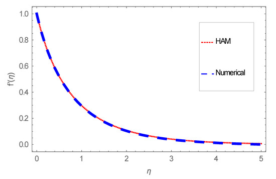
Figure 2.
Dual solution for velocity field.
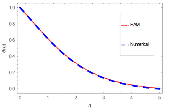
Figure 3.
Dual solution for temperature field.
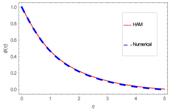
Figure 4.
Dual solution for concentration field.
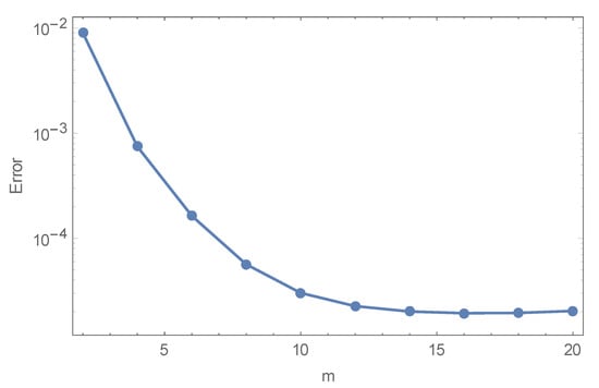
Figure 5.
Residual error via order of approximation.
4. Discussion
Noticeable characteristics of against drag force, , Nusselt number , Sherwood number , fluid velocity , thermal distribution and solutal distribution are explained and plotted in Figure 6, Figure 7, Figure 8, Figure 9, Figure 10, Figure 11, Figure 12, Figure 13, Figure 14, Figure 15, Figure 16, Figure 17, Figure 18, Figure 19, Figure 20, Figure 21, Figure 22, Figure 23, Figure 24, Figure 25, Figure 26, Figure 27, Figure 28, Figure 29, Figure 30, Figure 31, Figure 32, Figure 33 and Figure 34.
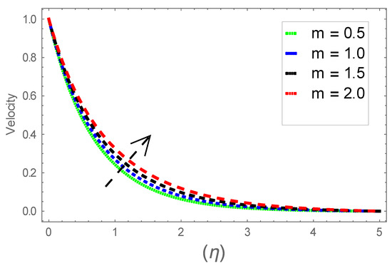
Figure 6.
Consequence of via .
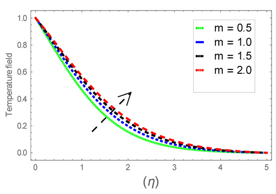
Figure 7.
Consequence of via .
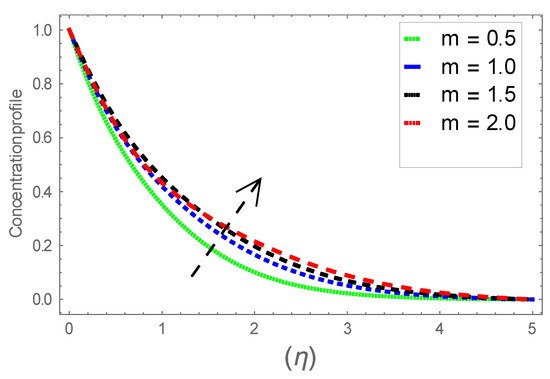
Figure 8.
Consequence of via .
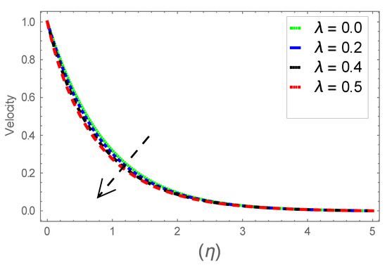
Figure 9.
Consequence of via .
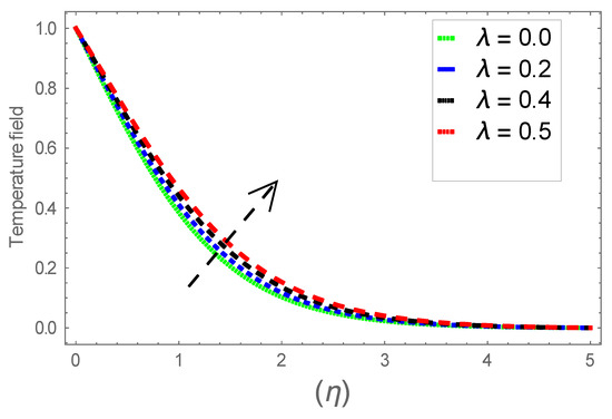
Figure 10.
Consequence of via .
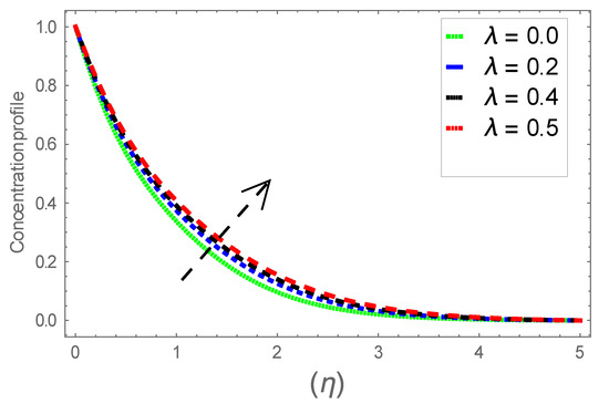
Figure 11.
Consequence of via .
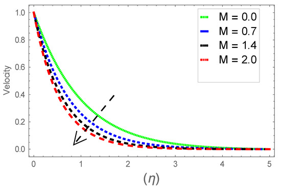
Figure 12.
Consequence of via .
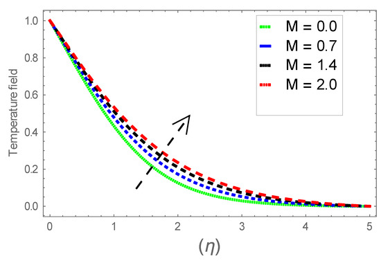
Figure 13.
Consequence of via .
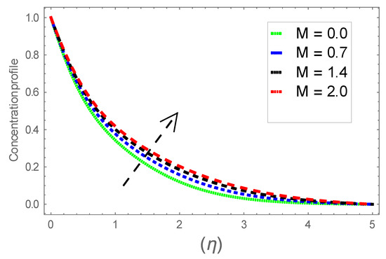
Figure 14.
Consequence of via .
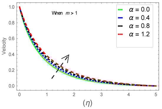
Figure 15.
Consequence of via .
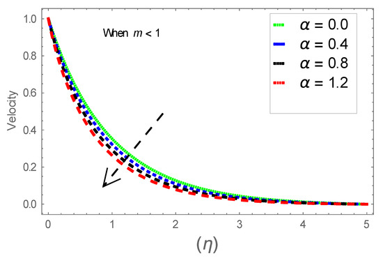
Figure 16.
Consequence of via .
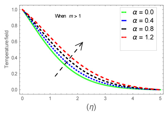
Figure 17.
Consequence of via .
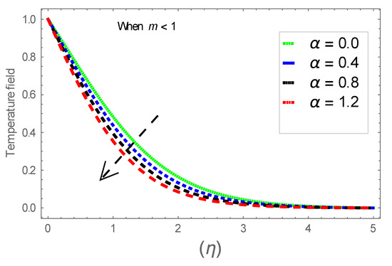
Figure 18.
Consequence of via .
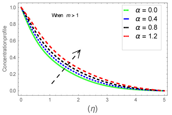
Figure 19.
Consequence of via .
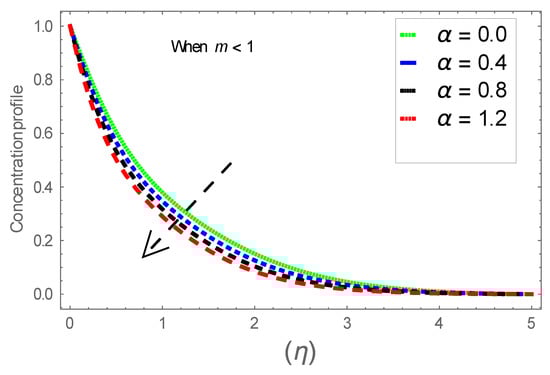
Figure 20.
Consequence of via .
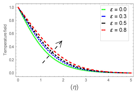
Figure 21.
Consequence of via .
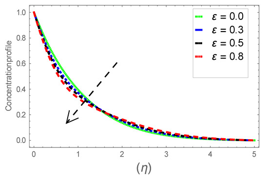
Figure 22.
Consequence of via .
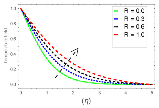
Figure 23.
Consequence of via .
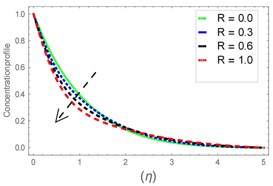
Figure 24.
Consequence of via .
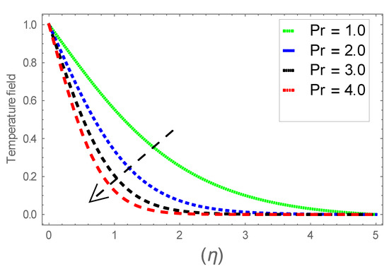
Figure 25.
Consequence of via .
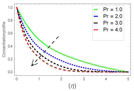
Figure 26.
Consequence of via .
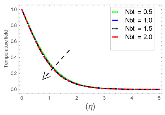
Figure 27.
Consequence of via .
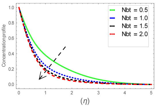
Figure 28.
Consequence of via .
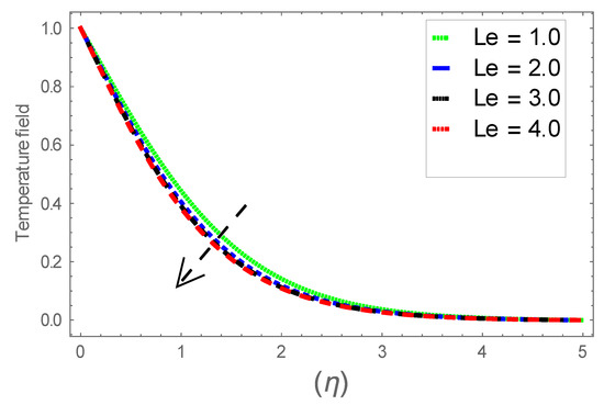
Figure 29.
Consequence of via .
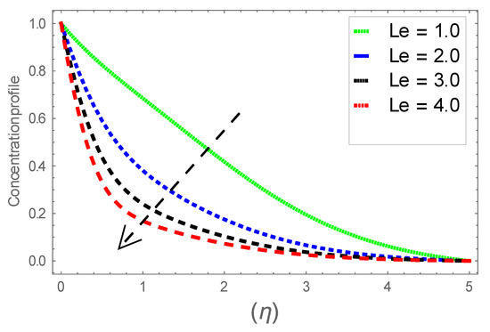
Figure 30.
Consequence of via .
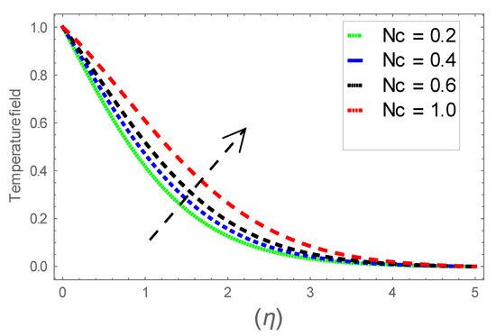
Figure 31.
Consequence of via .
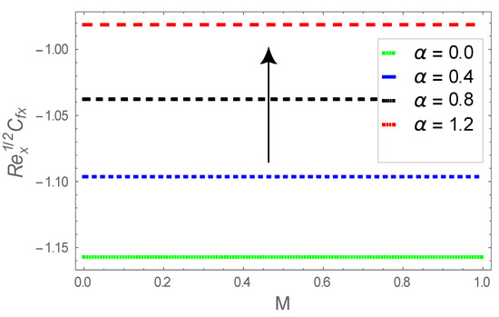
Figure 32.
Consequence of via .
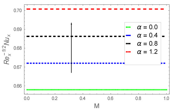
Figure 33.
Consequence of via .
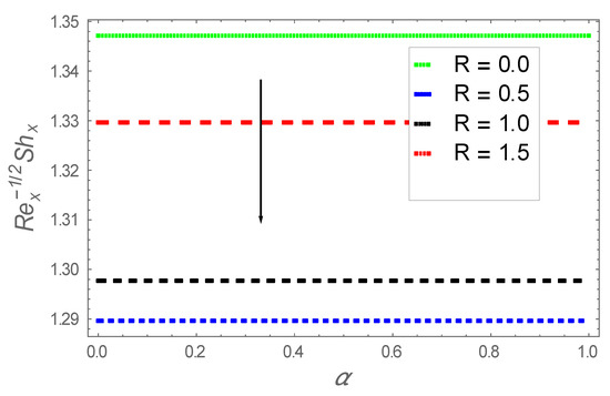
Figure 34.
Consequence of via .
Figure 6, Figure 7 and Figure 8 explain the attributes of velocity power index factor on . As anticipated, velocity, temperature and concentration fields are augmented subject to increment in . In consequence, momentum boundary layer thickness and thermal boundary layer thickness dwindles to higher values of . The contribution of Williamson parameter on are evaluated through Figure 9, Figure 10 and Figure 11. Here, in Figure 6, we found lower subject to increment in . Clearly, are the augmenting function of Williamson parameter. In reality, heat transference boosts through larger . Consequently, the solutal field escalates. Attributes of magnetic field influence on velocity, thermal and solutal fields are interpreted in Figure 12, Figure 13 and Figure 14. Clearly, Figure 12 unveils that velocity diminishes subject to boosts through larger . Physically, as escalates, fluid viscosity increases due to Lorentz force upsurges when is augmented. Moreover, this force has a resistive nature which controls fluid motion. It is significant interest that yield stress of the fluid can be measured and controlled correctly by changing effect of magnetic parameter. In consequence, the capacity of fluid to transmit force can be measured through an electromagnet which gives numerous possible control-based utilizations, which include MHD power generation, MHD ion propulsion, electromagnetic casting of metals, and many more. Figure 13 depicts variation in thermal field subject to higher . One can perceive that it is an augmenting function of . In reality, heat transference boosts through larger magnetic parameter. Consequently, it escalates . This reality lies in thermal energy dissipation due to applied magnetic field. Solutal field curves for are revealed in Figure 14. Clearly, is augmenting function of . In reality, when the magnetic field upsurges due to which fluid nanoparticles diffuse rapidly into the neighboring layers. Accordingly, rises. The contribution of wall thickness factor on are evaluated through Figure 15, Figure 16, Figure 17, Figure 18, Figure 19 and Figure 20. As anticipated, fluid velocity near to the plate dwindles subject to increment for and escalates for noticed in Figure 15 and Figure 16. Thermal field curves diminish near the plate for and augments for boosts through larger shown in Figure 17 and Figure 18. Solutal field boundary layer diminishes when however, reverse appearances are found for subject to larger wall thickness parameter perceived in Figure 19 and Figure 20. Figure 21 and Figure 22 emphasize variable thermal conductivity parameter impact on thermal field and solutal profile . Here, the thermal field curves upsurge when thermal conductivity augmented. In consequence, rises. However, reverse appearances are perceived for larger conductivity parameter in solutal field. Figure 23 explains variations in subjected to radiation parameter . This figure discloses augmentation for larger . In fact, working fluid achieves extra heat subject to radiation factor. In consequence, rises. Attributes of radiation factor on are interpreted in Figure 24. Clearly, diminishes when is augmented. The contribution of Prandtl number on is evaluated through Figure 25. Thermal diffusivity reduces when upsurges. Hence, thermal field decays. The contribution of curves for estimations are designed in Figure 26. Higher/larger Prandtl number estimations yield declines in . In reality, mass diffusivity reduces when is increased. Thus, diminishes. The contribution of on thermal field and solutal field curves are evaluated through Figure 27 and Figure 28. Thermal diffusivity reduces when upsurges. Hence, thermal field decays. In consequences, thermal boundary layer thickness diminishes. The solutal field reduces significantly subject to increment in . As is defined as the ratio of Brownian diffusivity to thermophoretic diffusivities. An upsurge in factor reasons for larger activity of nanoparticles in side base fluid. Attributes of Lewis number on thermal field and solutal field are interpreted in Figure 29 and Figure 30. Clearly, reduces when is augmented. Thus, thermal boundary layer thickness diminishes with upsurge in . Effect of Lewis number on solutal field is disclosed in Figure 30. Here, reduces versus higher estimations of factor. Figure 31 depicts variations in thermal field subjected to nanofluid heat capacity parameter . This figure discloses augmentation for higher . In fact, working nanofluid gets extra heat subject to larger parameter. In consequence, boundary layer thickness enhances.
Figure 32 emphasize impacts on . Here, upsurges when and are augmented. However, reverse features are found for larger values of . The attributes of influences on are elaborated in Figure 33. This figure confirms that upsurges subject to are enlarged. Influence of on are shown in Figure 34. The local Sherwood number, diminishes subject to increment in these parameters.
5. Closing Remarks
In this study, various aspects of heat transference and radiation effects on hydromagnetic boundary layer Williamson nanofluid flow in view of stretchable surface along with variable thickness and variable thermal conductivity characteristics have been analyzed. A computational numerical algorithm is employed to accomplish convergent solutions. We witnessed notable features through abovementioned investigation:
- It is perceived that velocity field diminishes when wall thickness factor augments for and reverse trends noticed in when .
- Thermal and solutal fields upsurge subject to increment in and diminishes with higher .
- An increment in parameter yields decays in and escalates thermal and concentration fields.
- Variable thermal conductivity parameter diminishes heat transfer coefficient .
- Sherwood number diminishes subject to increment in .
Author Contributions
Conceptualization, H.U.R. and S.I.; methodology, H.U.R.; software, H.U.R. and K.S.N.; validation, S.I., K.S.N., N.A.A., M.Z. and H.U.R.; formal analysis, K.S.N.; investigation, H.U.R.; writing—original draft preparation: H.U.R. and S.I.; writing—review and editing, H.U.R., K.S.N., N.A.A., M.Z.; All authors have read and agreed to the published version of the manuscript.
Funding
The authors extend their appreciation to the Deanship of Scientific Research at King Khalid University for funding this work through Research Group Program under grant No. RGP. 2/51/42. Nawal A. Alshehri acknowledges Taif University Researchers Supporting Project number (TURSP-2020/247), Taif University, Taif, Saudi Arabia.
Institutional Review Board Statement
Not applicable.
Informed Consent Statement
Not applicable.
Data Availability Statement
No data used or generated in this study.
Conflicts of Interest
The authors declare no conflict of interest.
References
- Choi, S.U.S.; Eastman, J. Enhancing thermal conductivity of fluids with nanoparticle. Master Sci. 1995, 231, 99–105. [Google Scholar]
- Buongiorno, J. Convective transport in nanofluids. ASME J. Heat Transf. 2006, 128, 240–250. [Google Scholar] [CrossRef]
- Daungthongsuk, W.; Wongwises, S.A. Critical review of convective heat transfer nanofluids. Renew. Sustain. Eng. Rev. 2007, 11, 797–817. [Google Scholar] [CrossRef]
- Wang, X.Q.; Mujumdar, A.S. A review on nanofluids part I: Theoretical and numerical investigations. Braz. J. Chem. Eng. 2008, 25, 613–630. [Google Scholar] [CrossRef]
- Wang, X.Q.; Mujumdar, A.S. A review on nanofluids part II: Experiments and applications. Braz. J. Chem. Eng. 2008, 25, 631–648. [Google Scholar] [CrossRef]
- Kakac, S.; Pramuanjaroenkij, A. Review of convective heat transfer enhancement with nanofluids. Int. J. Heat Mass Transf. 2009, 52, 3187–3196. [Google Scholar] [CrossRef]
- Ibrahim, W.; Gamachu, D. Nonlinear convection flow of Williamson nanofluid past a radially stretching surface. AIP Adv. 2019, 9. [Google Scholar] [CrossRef]
- Ibrahim, W.; Negera, M. Viscous dissipation effect on Williamson nanofluid over stretching/shrinking wedge with thermal radiation and chemical reaction. J. Phys. Commun. 2020, 4, 045015. [Google Scholar] [CrossRef]
- Ibrahim, W.; Negera, M. The investigation of MHD Williamson nanofluid over stretching cylinder with the effect of activation energy. Adv. Math. Phys. 2020, 2020, 9523630. [Google Scholar] [CrossRef]
- Yusuf, T.A.; Adesanya, S.O.; Gbadeyan, J.A. Entropy generation in MHD Williamson nanofluid over a convectively heated stretching plate with chemical reaction. Heat Transfer 2020, 49, 1982–1999. [Google Scholar] [CrossRef]
- Aldabesh, A.; Hussain, M.; Khan, N.; Riahi, A.; Khan, S.; Tlili, I. Thermal variable conductivity features in Buongiorno nanofluid model between parallel stretching disks: Improving energy system efficiency. Case Stud. Therm. Eng. 2021, 23. [Google Scholar] [CrossRef]
- Alhamaly, A.S.; Khan, M.; Shuja, S.Z.; Yilbas, B.S.; Al-Qahtani, H. Axisymmetric stagnation point flow on linearly stretching surfaces and heat transfer: Nanofluid with variable physical properties. Case Stud. Therm. Eng. 2021, 24. [Google Scholar] [CrossRef]
- Ramesh, G.K.; Gireesha, B.J.; Kumara, B.C.; Gorla, R.S. MHD stagnation point flow of nanofluid towards a stretching surface with variable thickness and thermal radiation. J. Nanofluids 2015, 4, 247–253. [Google Scholar] [CrossRef]
- Srinivasulu, T.; Goud, B.S. Effect of inclined magnetic field on flow, heat and mass transfer of Williamson nanofluid over a stretching sheet. Case Stud. Therm. Eng. 2021, 23, 100819. [Google Scholar] [CrossRef]
- Reddy, Y.R.; Rao, V.S.; Kumar, M.A. Effect of heat generation/absorption on MHD copper-water nanofluid flow over a non-linear stretching/shrinking sheet. AIP Conf. Proc. 2020, 2246. [Google Scholar] [CrossRef]
- Nayak, M.K.; Shaw, S.; Chamkha, S.J. 3D MHD free convective stretched flow of a radiative nanofluid inspired by variable magnetic field. Arab. J. Sci. Eng. 2019, 44, 1269–1282. [Google Scholar] [CrossRef]
- Williamson, R.V. The flow of pseudo plastic materials. Ind. Eng. Chem. 1929, 21, 1108–1111. [Google Scholar] [CrossRef]
- Rasheed, H.; AL-Zubaidi, A.; Islam, S.; Saleem, S.; Khan, Z.; Khan, W. Effects of joule heating and viscous dissipation on magnetohydrodynamic boundary layer flow of Jeffrey nanofluid over a vertically stretching cylinder. Coatings 2021, 11, 353. [Google Scholar] [CrossRef]
- Ibrahim, W.; Negera, M. Melting and viscous dissipation effect on upper-convected Maxwell and Williamson nanofluid. Eng. Rep. 2020, 2. [Google Scholar] [CrossRef]
- Vasudev, C.; Rao, U.R.; Reddy, M.V.S.; Rao, G.P. Peristaltic Pumping of Williamson fluid through a porous medium in a horizontal channel with heat transfer. Am. J. Sci. Ind. Res. 2010, 1, 656–666. [Google Scholar] [CrossRef]
- Nadeem, S.; Hussain, S.T. Flow and heat transfer analysis of Williamson nanofluid. Appl. Nanosci. 2014, 4, 1005–1012. [Google Scholar] [CrossRef]
- Gorla, R.S.R.; Gireesha, B.J. Dual solutions for stagnation-point flow and convective heat transfer of a Williamson nanofluid past a stretching/shrinking sheet. Heat Mass Transf. 2016, 52, 1153–1162. [Google Scholar] [CrossRef]
- Abbas, Z.; Rafiq, M.Y.; Alshomrani, A.S.; Ullah, M.Z. Analysis of entropy generation on peristaltic phenomena of MHD slip flow of viscous fluid in a diverging tube. Case Stud. Therm. Eng. 2021, 23. [Google Scholar] [CrossRef]
- Fang, T.; Zhang, J.; Zhong, Y. Boundary layer flow over a stretching sheet with variable thickness. Appl. Math. Comput. 2012, 218, 7241–7252. [Google Scholar] [CrossRef]
- Subhashini, S.V.; Sumathi, R.; Pop, I. Dual solutions in a thermal diffusive flow over a stretching sheet with variable thickness. Int. Comput. Heat Mass Transf. 2013, 48, 61–66. [Google Scholar] [CrossRef]
- Khader, M.M.; Meghad, M.A. Differential transformation method for studying flow and heat transfer due to stretching sheet embedded in porous medium with variable thickness, variable thermal conductivity, and thermal radiation. Appl. Math. Mech. Engl. Ed. 2014, 35, 1387–1400. [Google Scholar] [CrossRef]
- Nayak, M.K.; Shaw, S.; Makinde, O.D. Chemically reacting and radiating nanofluid flow past an exponentially stretching sheet in a porous medium. Indian J. Pure Appl. Phys. 2018, 56, 773–786. [Google Scholar]
- Sachin, S.; Motsa, S.S.; Sibanda, P. Magnetic field and viscous dissipation effect on bioconvection in a permeable sphere embedded in a porous medium with a nanofluid containing gyrotactic micro-organisms. Heat Transfer Asian Res. 2018, 47, 718–734. [Google Scholar]
- Sachin, S.; Motsa, S.S.; Sibanda, P. Nanofluid flow over three different geometries under viscous dissipation and thermal radiation using the local linearization method. Heat Transfer Asian Res. 2019, 48, 2370–2386. [Google Scholar]
- Rasheed, H.; Khan, Z.; Islam, S.; Khan, I.; Guirao, J.L.G.; Khan, W. Investigation of two-dimensional viscoelastic fluid with nonuniform heat generation over permeable stretching sheet with slip condition. Complexity 2019, 2019, 3121896. [Google Scholar] [CrossRef]
- Rasheed, H.; Khan, Z.; Khan, I.; Ching, D.L.C.; Nisar, K.S. Numerical and analytical investigation of an unsteady thin film nanofluid flow over an angular surface. Processes 2019, 7, 486. [Google Scholar] [CrossRef]
- Chaim, T.C. Heat transfer in a fluid with variable thermal conductivity over a linearly stretching sheet. Acta Mech. 1998, 129, 63–72. [Google Scholar] [CrossRef]
Publisher’s Note: MDPI stays neutral with regard to jurisdictional claims in published maps and institutional affiliations. |
© 2021 by the authors. Licensee MDPI, Basel, Switzerland. This article is an open access article distributed under the terms and conditions of the Creative Commons Attribution (CC BY) license (https://creativecommons.org/licenses/by/4.0/).