Framework for Mitigation of Welding Induced Distortion through Response Surface Method and Reinforcement Learning

Abstract

Welding induced distortion causes dimensional inaccuracies in parts being produced and assembly fit-up problems during manufacturing. In this study, a framework is proposed to mitigate weld distortion at the design stage. A sequential approach is adopted to optimize the welding process. In the first phase, welding process parameters are optimized through the response surface method. The effect of these parameters on the overall distortion of the welded part is observed by a simulation of the welding process. In the second phase, the weld sequence is optimized using the optimum weld parameters. A reinforcement learning-based Q-learning technique is used to select the optimum welding path by sequential observation of weld distortion at each segment being welded. The optimum process parameters and weld path sequence have been selected for 3 mm steel plates having a lap joint configuration and a 2 mm vent panel with a butt joint configuration. It is concluded that the combination of the optimum welding parameters and welding sequence yields minimum distortion. By applying this framework, a reduction of 19% is observed in overall welding induced distortion.

1. Introduction

The control, prediction, and optimization of distortion produced during welding need to be addressed at the design stage to improve dimensional accuracies of the part being manufactured and to avoid misalignment of mating parts during assembly. Combined optimization of welding process parameters and the welding sequence is needed to mitigate distortion produced during welding. Yi et al. [1] conducted an experimental and numerical investigation on welding induced distortion. The authors concluded in their research that welding parameters and the welding path sequence both influence the overall distortion produced during welding. Daniyan et al. [2] discussed the use of the response surface method and Taguchi methods for optimization of weld process parameters, i.e., welding current, voltage, speed, and arc length. The objective of their study was to reduce welding distortion by searching for the optimum weld parameters. The response surface method was used by Liu et al. [3] for optimization of laser welding of dissimilar metals. They used central composite design to construct the design of the experiment (DOE) matrix. Zuo et al. [4] used the response surface method for optimization of weld process parameters in friction stir spot welding. They used Box–Behnken design to find the relationship between different process parameters. The response surface method has also been used in combination with other evolutionary algorithms. Srichok et al. [5] used the response surface method (RSM) and modified differential evolution (MDE) to optimize the friction stir welding process. They concluded that the RSM–MDE approach increased the joint tensile strength by 1.48%. Sulaiman et al. [6] studied the effect of welding parameters, current, voltage, speed, wire feed, and shielding gas on distortion produced in T and butt-jointed steel plates. Kshirsagar et al. [7] optimized TIG welding parameters using the Nelder–Mead algorithm. They used welding current and speed as the main input parameters to optimize weld bead geometry. Tomków et al. [8] discussed the influence of tack weld distribution and the welding sequence on welding induced distortion. Weld sequence optimization is treated as a separate subject. M. Asadi et al. [9] proposed weld sequence optimization of panel structures using the joint rigidity method. In this research, control of welding induced distortion is managed at the design stage with the use of finite element simulation. The criterion for selecting the optimum welding path is based on the joint’s rigidity. Hdz et al. [10] proposed welding sequence optimization through a Q-learning algorithm. Q-learning is a subclass of reinforcement learning, which is an established branch of machine learning. In reinforcement learning, an agent that is a robot finds the optimum path in a confined environment by advancing through different states within that environment. To achieve a certain goal, the agent gets a reward at each step during the pathfinding process. The reward-based system is sequential and targeted to achieve the main objective. The authors have drawn an analogy between the agent, in this case, the welding robot, and states that are weld segments. Whenever the welding robot welds a weld segment it gets a reward according to the reciprocal of the amount of distortion produced during welding. The lesser the distortion, the greater will be the reward. Artificial intelligence was used by Yang et al. [11], who used a deep learning algorithm for visual inspection of the laser welding process.

Welding parameter optimization and welding sequence optimization are both combinatorial problems in nature. If there are $k$number of welding parameters under study and each parameter has two levels, the full factorial design will consist of $2^k$ experiments. Similarly, for the welding sequence, the number of welding sequence combinations ($N$) are decided by $N = n^r \times r!$ where $n$ is the number of welding directions and$r$ is the number of weld passes. If welding parameters and sequence optimization are treated simultaneously, the number of experiments increases exponentially. Islam et al. [12] proposed a FEM–RSM–GA-based approach for minimization of welding distortion at the design stage. The welding process parameters and weld sequence are simultaneously studied in this work. The optimum weld parameters are selected by the response surface method and further optimized by a genetic algorithm (GA). The authors used a steel sample with a lap joint having two weld segments that can be welded in six possible weld sequences with two welding robots. During the last step of optimization, i.e., GA-based optimization, only one weld sequence was used, and the focus of the research was to find the optimum process parameters. It took 75 weld simulations to achieve the required goal.

The balancing of the experiment matrix is another problem that researchers have faced while addressing the optimization of the complete weld process. The number of weld parameters selected for optimization study ranges from three to four parameters in one optimization run, while the number of weld segments ranges from four to a few hundred. Therefore, the total number of experiments required to find the optimum solution increases exponentially. As an example, consider three welding parameters, i.e., welding current, speed, and torch angle, with 3 levels for each parameter; for example, the welding current has three levels of 100, 120, and 140 A, and the same goes for the other two parameters. A central composite design for this type of experiment requires nine experimental runs with an additional three central runs for error detection. In each experimental run, a different level of weld parameter is used. Taguchi L9 orthogonal array will also require nine experiments. In this scenario, if a weld sequence is added with the optimization study having four weld segments to be welded in two weld directions, the number of weld sequences will be $2^4 \times 4!$. A total of 384 weld sequences need to be investigated. It is therefore not feasible to search for optimum weld parameters along with an optimum weld sequence with the design of experiment approach. Other optimization techniques, such as GA and Artificial Neural Networks, have been used by various researchers. Kim [13] used GA and the traveling salesman problem to solve single pass multi-weld sequence optimization. The genetic algorithm searches the whole design space with a set of solutions called chromosomes. The solutions are modified and updated based on crossover and mutation. There are two problems with this kind of heuristic: in a welding optimization problem, one might come across a solution set that is not feasible or practically applicable, i.e., a combination of welding speed, current, and voltage at which welding of the base material to be tested is not possible at all. The other problem is in searching the whole space for a feasible set of solutions. Simulation of the welding process requires extensive time, and hence computational cost, for a single run of a solution set. The computational requirement of welding process simulation by finite element analysis is well known and has been reported in various research works. Deshpande [14] discussed the comparison of commercial software for simulation of the welding process. A single weld in a plate size of 100 mm × 50 mm took 160 min for complete simulation. Mitra [15] reported the computational time, the type of processor, and the RAM used in simulating the welding process. It took 49.96 h for 600 weld beads using a 3.6 GHz Intel Xeon processor with 48 GB of RAM. Goldak and Asadi [16] studied an industrial problem with 24 weld sub-passes. The design of experiment approach was used to optimize the weld sequence in 32 runs. It took 16 days of computational time by running eight projects at a time on a dual processor with eight cores. In the present research, a framework is proposed to minimize welding induced distortion by finding a combination of the optimum weld parameters and optimum weld sequence. It is a sequential approach in which optimum weld parameters are selected using the response surface method. In the second phase, weld sequence optimization is achieved by the reinforcement learning-based technique, Q-learning. During the weld parameter optimization, the length of the weld bead is limited to a shorter length with a single pass. The present study combines both weld parameter optimization and weld sequence optimization in a framework. However, the scope of this study does not include the influence of tack weld distribution. The framework of the complete optimization process is discussed in the next section.

2. Framework of Welding Optimization

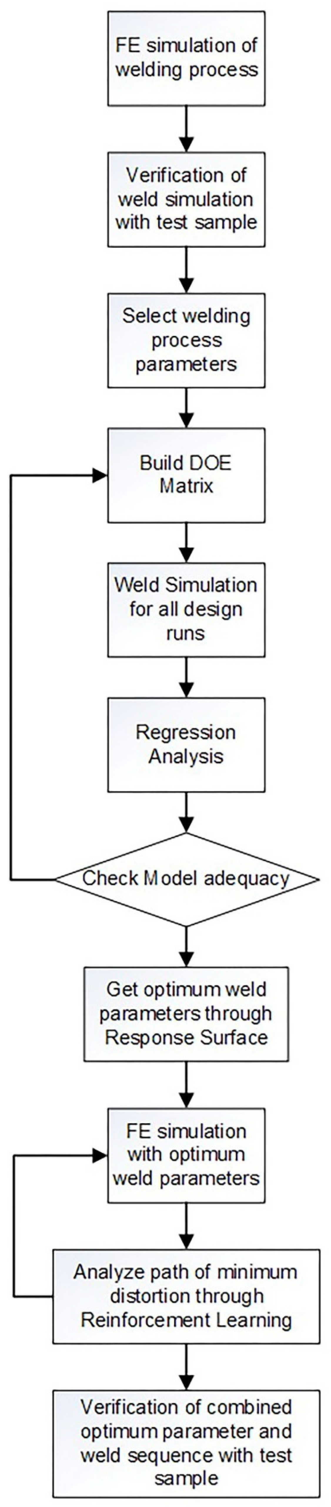
A flow chart of the complete welding optimization process is given in Figure 1. The whole process can be divided into two phases. The first phase focuses on optimization of weld parameters. The weld sequence is kept constant during this phase. After selection of the optimum weld parameters, welding sequence optimization is carried out. The first step of weld parameter optimization constitutes running the weld simulation with random weld parameters. A test sample is prepared to verify the simulation results. The finite element model used in weld simulation is calibrated by comparison of distortion results with the test sample. Selection of critical weld parameters that influence distortion induced during welding is completed at this stage. In this research, the three weld parameters of welding current, speed, and voltage are selected. In terms of the design of the experiment study, these parameters are called factors and the response to be studied is the overall distortion produced during welding. The next step is to select the level of each factor and to fill the design of the experiment table. A detailed discussion on the selection of the experimental design matrix is presented in Section 4. The third step is to simulate the welding process by changing the parameter values.

The results of experiments, i.e., distortion produced during welding, are stored in the response column of the DOE matrix. In the fourth step, regression analysis is performed to check the estimate of error, interactions between factors of the model, and the quadratic effects or curvature. In the next step, response surface and 2D contour plots of two-factor interaction are generated. Further optimization of weld parameters is achieved by using the regression equation. After finding the optimum weld parameters, the second phase of weld sequence optimization starts. The start and end positions of weld segments are defined as states, and the action, i.e., welding, is performed between these states. On moving from one state to the next neighboring state, the welding process is simulated and the distortion produced for this action is noted. A reward is generated based on the reciprocal of distortion produced. A state value function is evaluated based on reward. After several iterations, the optimum weld sequence is selected based on the highest reward and state value function.

In the last step, weld simulation of a single weld segment is performed one at a time, unlike optimization techniques such as the GA where a complete solution is required to be compared between a population. This saves the computational cost of the whole process. The optimum weld sequence is compared with other weld sequences and the same weld sequence with different weld parameters to verify the results of the process. The final verification is performed by comparison of simulation results with experimentally measured distortion in the test sample. The test sample is prepared by using optimum weld parameters and weld sequence. The process of weld simulation by finite element analysis is explained in the next section.

3. Welding Simulation

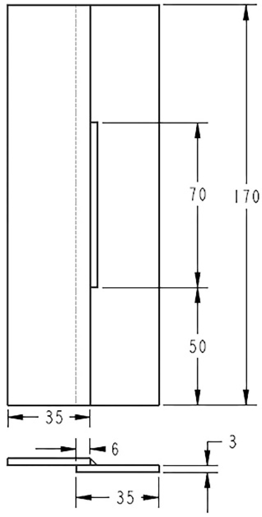
The test sample chosen for simulation of the welding process is 3 mm ASTM A36 steel. This steel grade is used extensively in a wide range of engineering applications [17]. Dimensions (in millimeters) of the sample are given in Figure 2. Two plates of size 35 mm × 170 mm are welded in a lap joint configuration with an overlap of 6 mm.

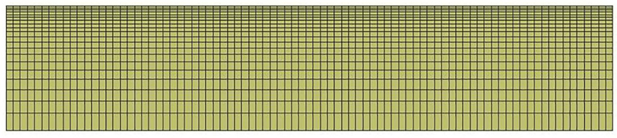
The length of the weld bead, which is placed in the middle of the plates for symmetry, is 70 mm. The biased meshing of both plates is implemented with refinement near the welding edges. A total of 3400 elements are used in one plate, as shown in Figure 3. Solid 8-node brick elements are used to avoid convergence problems during the solution phase. A fillet weld of 3 mm leg length is included in the FE model. The mechanical boundary conditions include clamps on the four corners of the plate and support at the bottom of the plate. Weld simulation analysis is performed in two parts. In the first part, transient thermal analysis is performed. The temperature dependent thermal and mechanical properties (thermal conductivity, specific heat, elastic modulus, yield strength, thermal expansion coefficient) used in the simulations are extracted from the work of Chang et al. [17]. Heat is applied to the weld bead geometry using a double ellipsoidal heat source proposed by Goldak [18], with front side 2 mm, rear side 7.3 mm, width 3.7 mm, and depth 3 mm.

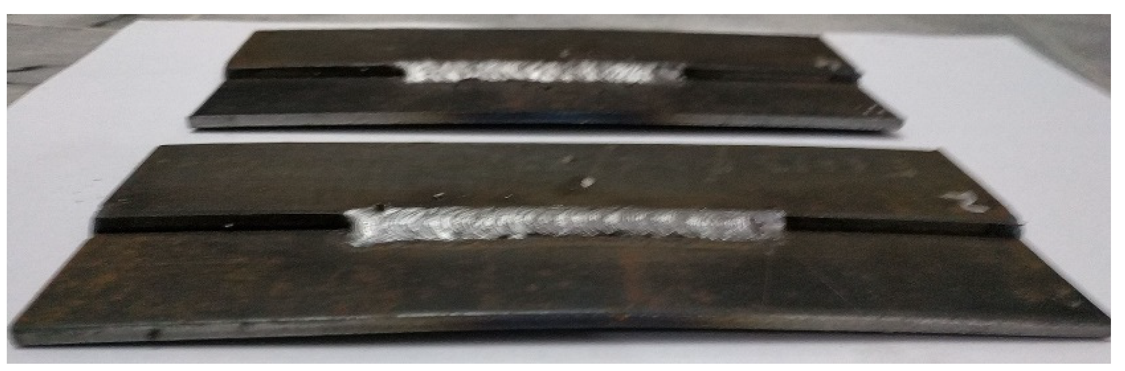
The moving heat source is translated in the weld direction. The concept of element birth and death is used to make the weld bead elements alive at the time of heat input in the weld zone. In the transient structural analysis, temperature history from the thermal analysis is used as the loads applied to the model. The focus of this weld simulation is to calculate the distortion produced during welding. To verify the result of welding analysis and to calibrate the heat source parameters, test samples are prepared from steel plates. A test sample is shown in Figure 4.

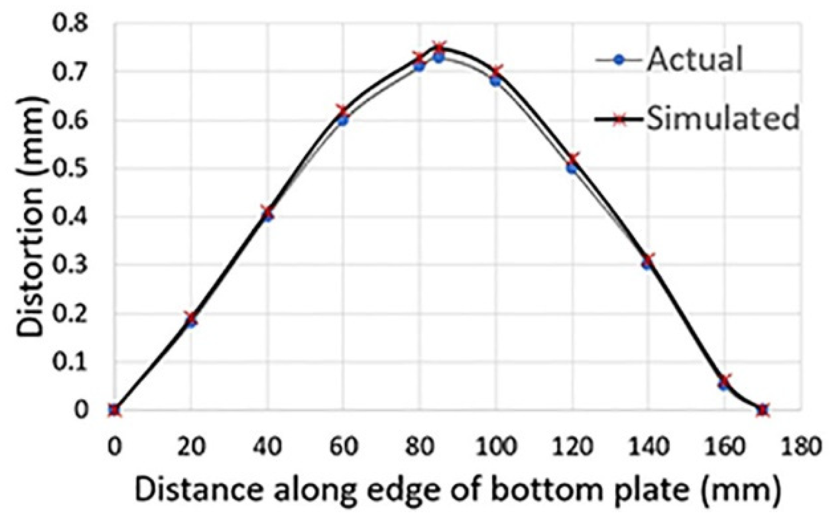
The samples are welded with the same configuration and parameters as used for the welding simulation. The distortion produced during welding is measured and the results are compared with simulated distortion values. Distortion is measured along the edge of the bottom plate because the maximum distortion was observed on that edge. These distortion values are measured using a coordinate measuring machine. The actual weld results are in close agreement with the simulated results. A graph of actual and simulated results along the edge of the bottom plate is shown in Figure 5.

The stage is set to use weld simulations to run the design of experiment procedure for weld parameter optimization.

4. Weld Parameter Optimization

In this research, the weld parameters selected are welding current, speed, and voltage. The combination of welding current and speed provides the heat in watts to produce sound welds. Welding speed in mm/s expresses the amount of heat the base metal receives during welding. All three factors are related to heat-input during the welding process. The amount of heat is related to temperature rise and variation within the base metal, which produces residual stress and distortion. Wahab et al. [19] have studied the influence of welding speed and current on the shape of weld pool geometry. Okano [20] developed an arc physics-based heat sourced model to study distortion produced during welding. The weld parameters used in this research are welding current, speed, and voltage. These parameters are varied to find the final distorted shape of the specimen. Guo et al. [21], in their experimental study on distortion measurement, related the longitudinal shrinkage in the base metal directly to heat input. The main factors of heat input are welding, current, speed, and voltage. The level of factors selected for the experimental run is another critical aspect of DOE. In this research, three levels of each factor are selected. To cover the entire design space, the highest and lowest levels selected should be the maximum current, the minimum current, the highest welding speed, the lowest welding speed, and so on. The combination of these extreme conditions produces unfeasible solutions. There might be an experimental run in which a combination of the highest welding current and highest voltage comes with the lowest speed. This combination will generate a high amount of heat which will be practically not possible. To overcome this situation, the response surface method technique is used. The first step in the response surface method is to select sets of parameters or factors with small increments. In the welding optimization case, if the welding current of 100 A is selected as a lower limit, the higher and middle terms will be selected in increments of 5 to 10 A. The three levels of current will then be 100, 105, and 110 A. The response surface method also defines a path of improvement for searching the optimum parameters. It is an iterative process: the factors are incremented in each iteration until the stationary point is reached.

4.1. DOE Matrix

The most popular design for fitting models in the response surface method is the central composite design (CCD) [22]. The central composite design consists of central runs at the extreme corners of the design space.

As an example, if +1 and −1 are the lowest and highest levels of two factors used, then the central composite design will consist of a combination of (−1−1), (−1+1), (+1−1), and (+1+1). The central run and axial run will be in between. In the systems in which extreme conditions need to be avoided, a modified version of central composite design, called the spherical CCD, is used. Spherical CCD is rotatable, which means the variation of every point that has the same distance from the center is the same. CCD is recommended for three to five central runs. Another design that has the property of rotatability is the Box–Behnken design. This design was initially proposed for three-level factor runs [22]. The Box–Behnken design is spherical, as the points to be tested for experiments lie in the middle of the cube and not at the corner, as is the case with CCD. The three factors with three levels at the stationary point used in this research are presented in

Table 1. DOE Matrix.

Experimental Run	${\mathit{X}}_{\mathbf{1}}$ = Current (A)	${\mathit{X}}_{\mathbf{2}}$ = Voltage (V)	${\mathit{X}}_{\mathbf{3}}$ = Speed (mm/s)
1	140	19	8.5
2	140	21	8.5
3	160	19	8.5
4	160	21	8.5
5	140	20	8
6	140	20	9
7	160	20	8
8	160	20	9
9	150	19	8
10	150	19	9
11	150	21	8
12	150	21	9
13	150	20	8.5
14	150	20	8.5
15	150	20	8.5

. This is a typical representation of a Box–Behnken design with three central runs.

In Figure 6, the design runs are shown on the respective axis in a cube. The bottom corner of the cube represents the lower levels of each factor. There are no experimental runs on the extreme corners of the cube.

The yellow dot on the front face of the cube represents the first experimental run, with welding current 140 A, voltage 19 V, and a welding speed of 8.5 mm/s. The blue dot represents the ninth experimental run in Table 1. The green dot represents the third experimental run, and the black dot represents the tenth experimental run. On the front face of the cube, welding voltage is constant during all four experiments, while welding speed and voltage vary from mid-point to the maximum level. The weld process simulation of each experiment is performed by finite element analysis. The distortion produced during welding is observed and analyzed with the help of regression analysis.

4.2. Regression Analysis

Regression analysis provides a mathematical model for interacting terms of factors under study. It also provides the path and step sizes for searching for the optimum solution. A linear model is used to find the path of steepest descent. At the stationary point, a full quadratic analysis is run. The mathematical model with interacting terms is given in Equation (1).

$$\begin{array}{c}Total Distortion = 34.1 - 0.383X_1 - 0.55X_2 - 0.10X_3 + 0.001443X_1{}^2 + 0.0143X_2{}^2\\ + 0.187X_3{}^2 + 0.00350X_1{X}_2 - 0.01350X_1{X}_3 - 0.0550X_2{X}_3\end{array}$$

(1)

In the above equation, variable $X_1$ is the current, $X_2$ is the voltage, and $X_3$ is speed. The coefficients of regression: ${\beta }_0$ is 34.1, ${\beta }_1$ is 0.383, ${\beta }_2$ is 0.55, and ${\beta }_3$ is 0.10, and so on. The interacting terms ${\beta }_{12}$, ${\beta }_{13}$, ${\beta }_{23}$ are also present in the equation. As explained in Section 4, all the factors, i.e., welding current, voltage, and speed contribute to the heat produced during welding, and hence are major contributors to the amount of distortion produced during welding. The interacting term $X_1{X}_2$, which is the product of current and voltage, if multiplied by arc efficiency gives the overall heat input of the welding process. Similarly, when this product is divided by the welding speed, it gives the amount of heat supplied per unit length in units of J/cm.

4.3. Response Surface

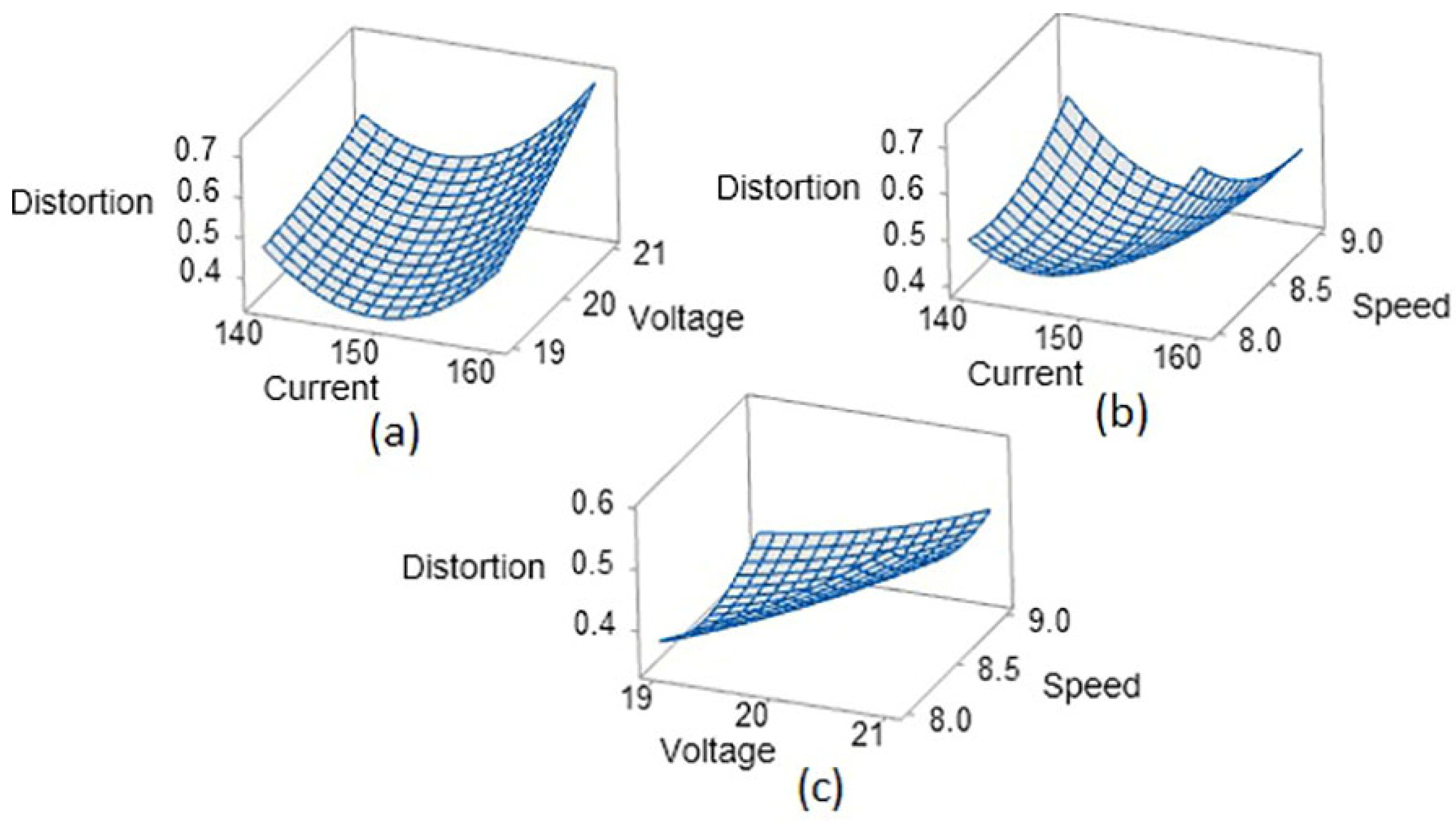
Response surfaces generated in the optimization study are given in Figure 7a–c. The maximum distortion produced during welding is plotted against the parameters of current, speed, and voltage. All three response surfaces show a saddle-like curve, because the main objective was to minimize the distortion. In Figure 7a, the distortion is minimum for the current of 150 A and a welding speed of 8.5 mm/s. The value of the distortion slightly increases on the lower current side, which is 140 A, and shows a substantial increase towards 160 A. In Figure 7b,c, it can be seen that a low voltage of 19 V produces a minimum distortion value.

4.4. Contour Plots and Optimization

The response surfaces give a general idea of the optimum value for each factor under study. Contour plots can be studied to find limits for each factor. Contour plots are 2D plots; therefore, for design optimization of three variables, contour plots of two variables can be generated by keeping the third variable constant.

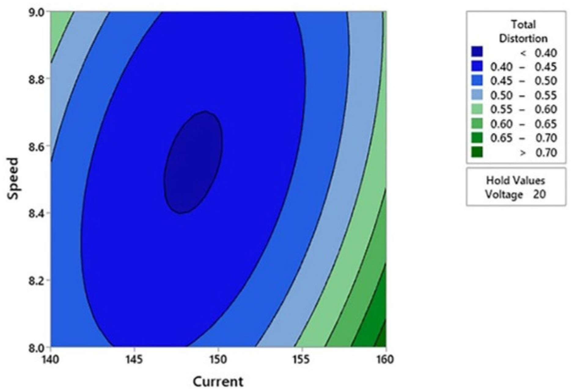
The minimum value of distortion observed in response surfaces, as shown in Figure 7, is less than 0.4 mm. The contour plot in Figure 8 shows that a distortion value of less than 0.4 mm can be achieved by setting the welding current between 147 and 150 A. The welding speed between 8.4 and 8.6 gives good results in terms of distortion produced. It can be observed from contour lines in Figure 8 that a value of current above 150 A will increase distortion from 0.5 to 0.7 mm. The contour plot, shown in Figure 9, is distortion vs. speed and voltage. It can be observed from this contour plot that at a welding speed of 8.5 mm/s, the voltage should be kept at a minimum of 19 V. The distortion can be minimized to 0.35 mm by reducing voltage. 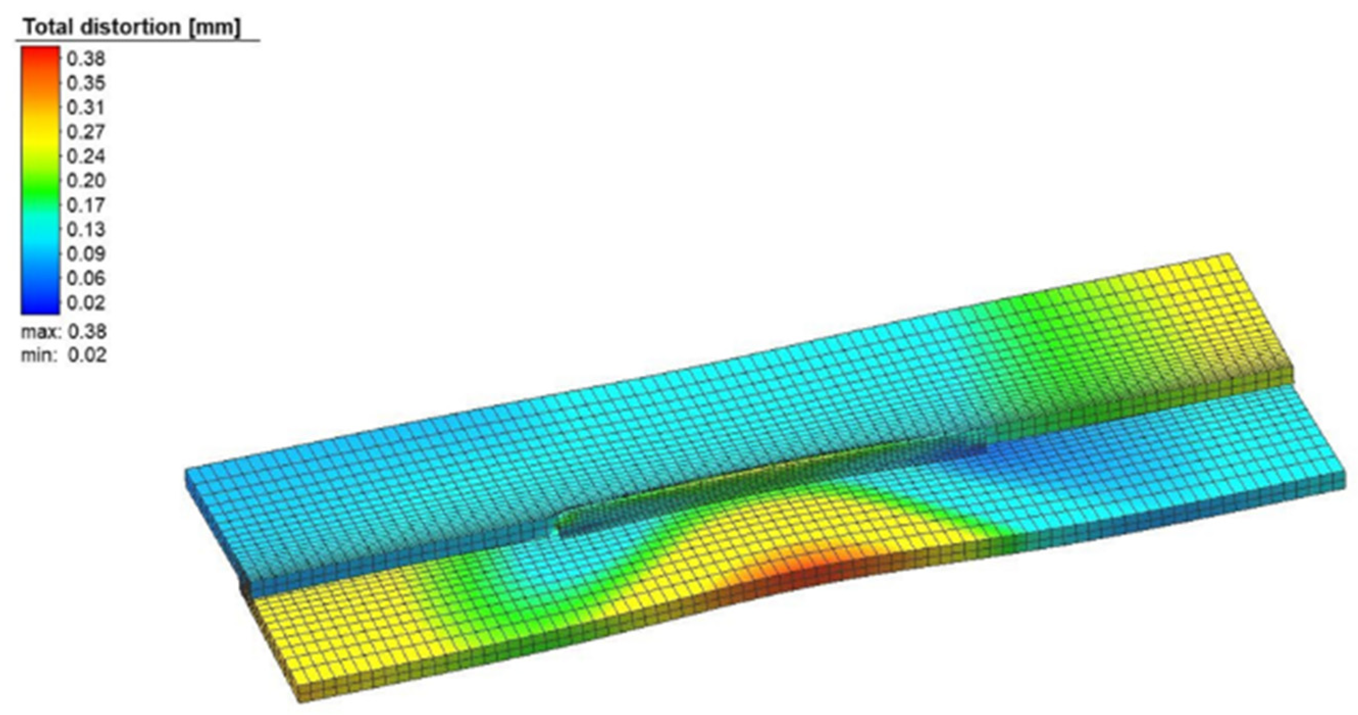The minimum distortion observed during all experimental runs, as per Table 1, was 0.4 mm. After studying contour plots, optimum parameters were selected, which are shown in

Table 2. Optimum weld parameters.

Current	Voltage	Speed
148 A	19 V	8.4 mm/s

. A weld simulation procedure is performed to test these parameters. The welding distortion observed is 0.38 mm. The result of the weld simulation with the final distorted shape is shown in Figure 10. The optimum weld parameters were utilized for the weld sequence optimization, to be discussed in the next section.

5. Weld Sequence Optimization

Weld sequence optimization involves selecting the optimum path from a combination of weld segments. In this research, Q-learning based optimization is used. It is based on the Markov reward process for decision making. An analogy between the artificial intelligence environment can easily be drawn for the welding process. In artificial intelligence, an agent, which is usually a robot, has to find the optimum path by moving from state to state within a certain environment. The movement from one state to another is called action. In the welding process, the welding robot changes position from one state, in this case, the start of the weld segment, to another state. The action performed is welding. The amount of welding induced distortion produced by this action gets a reward proportional to the reciprocal of distortion. If the probabilities or rewards are unknown, and the action to be taken is unknown, then this is a typical case of reinforcement learning [23]. Q-learning and artificial intelligence-based techniques have been used in the past for welding path optimization. Okumoto [24] used reinforcement learning to optimize the weld path sequence in ship hull block welding. The ship hull block has several closely knitted weld joints. The movement of the welding robot truck system to weld these joints was optimized using Q-learning. Recent research work includes a patent by Yoshida et al. [25], which uses reinforcement learning for monitoring and improving arc weld conditions. Hdz et al. [10] have used Q-learning for optimization of the weld sequence for weld distortion minimization. The Q-learning based algorithm was tested on a bracket assembly to find the optimum weld sequence which produced minimum distortion during welding. In the present research, a lap joint configuration is used for weld sequence optimization. The lap joint case is similar to the weld configuration used in weld parameter optimization.

5.1. Lap Joint Case Study

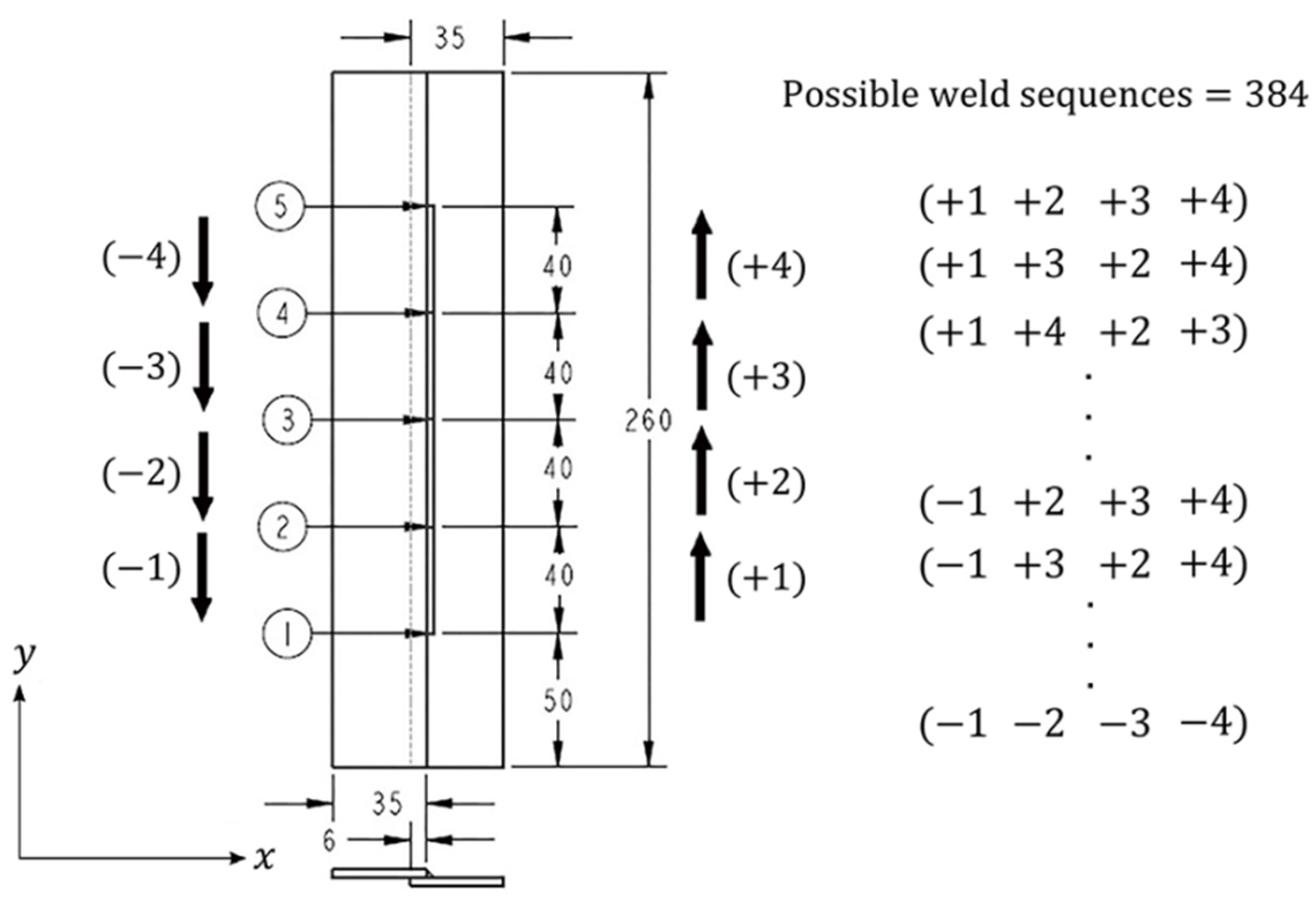
The weld configuration for sequence optimization is shown in Figure 11. Two steel plates of 3 mm thickness have an overlap of 6 mm. The overall length of the plate is 260 mm. Weld segments of 40 mm each are to be welded 50 mm from the edge of the plate.

The weld segments can be welded in two directions. The direction along the positive y-axis is represented by a ‘+’ sign, while the reverse or backward welding is represented by a ‘−’ sign. The total number of weld sequences N is given in Equation (2).

$$N = 2^4 \times 4! = 384$$

(2)

The computational time is 15 min for a welding simulation of a four-segment lap joint on a normal workstation (32 GB RAM Octa-core Processor). The total time required for exploration of all welding sequences for this simple case will be 96 h or 4 days. The numbers encircled in Figure 11 are the states, i.e., weld segment 2 is welded by moving the agent/welding robot from state 2 to state 3. The same weld segment can be welded by moving from state 3 to state 2. The programming steps for welding sequence optimization through the Q algorithm are given below.

Algorithm 1 Welding Sequence Optimization
	N = number of weld segments
	A = state action matrix
	C = coordinate matrix for each state
	α = learning rate
	γ = discount factor
1	initiate reward matrix$R = N \times N = 0$
2	initiate Q matrix$Q = N \times N = 0$
3	Initial value of maximum reward$R_{max} = 0$
4	for t = number of exploration iterations
5		generate random welding sequence
6		Store in A
7		if positive welding direction is selected
8			delete the corresponding negative direction
9		end
10		for$r = 1 to N$
11			calculate vector sum of last final state to next initial state using C matrix
12			Calculate reward and update R matrix
13		end
14		for$q = 1 to N$
15			Update Q matrix for every state action combination
16			$Q\left(s,a\right)\leftarrow Q\left(s,a\right)+\alpha \{R\left(s,a\right)+\gamma ·\underset{\stackrel{‛}{a}}{\max } Q(\stackrel{‛}{s},\stackrel{‛}{a})-Q\left(s,a\right)\}$
17		end
18		$R_{sum}$ = sum of all elements of matrix R
19		If$R_{sum}>R_{max}$
20			$R_{sum} = R_{max}$
21		end
22	end
23	for t = number of exploitation iterations
24		generate welding sequence based on maximum Q value
25		Repeat step 6 to 22
26	end
27	Plot (t,$R_{sum}$)

In generating a random welding sequence, a check is introduced in step 7 to delete the corresponding reverse state action, i.e., if the welding segment + 1 is selected then the reverse welding segment − 1 is deleted from the selection matrix. The reward for the transition from the current state to the next state is calculated by Equation (3).

$$R = \sqrt{{\left(C_{x1}-C_{x2}\right)}^2+{\left(C_{y1}-C_{y2}\right)}^2}$$

(3)

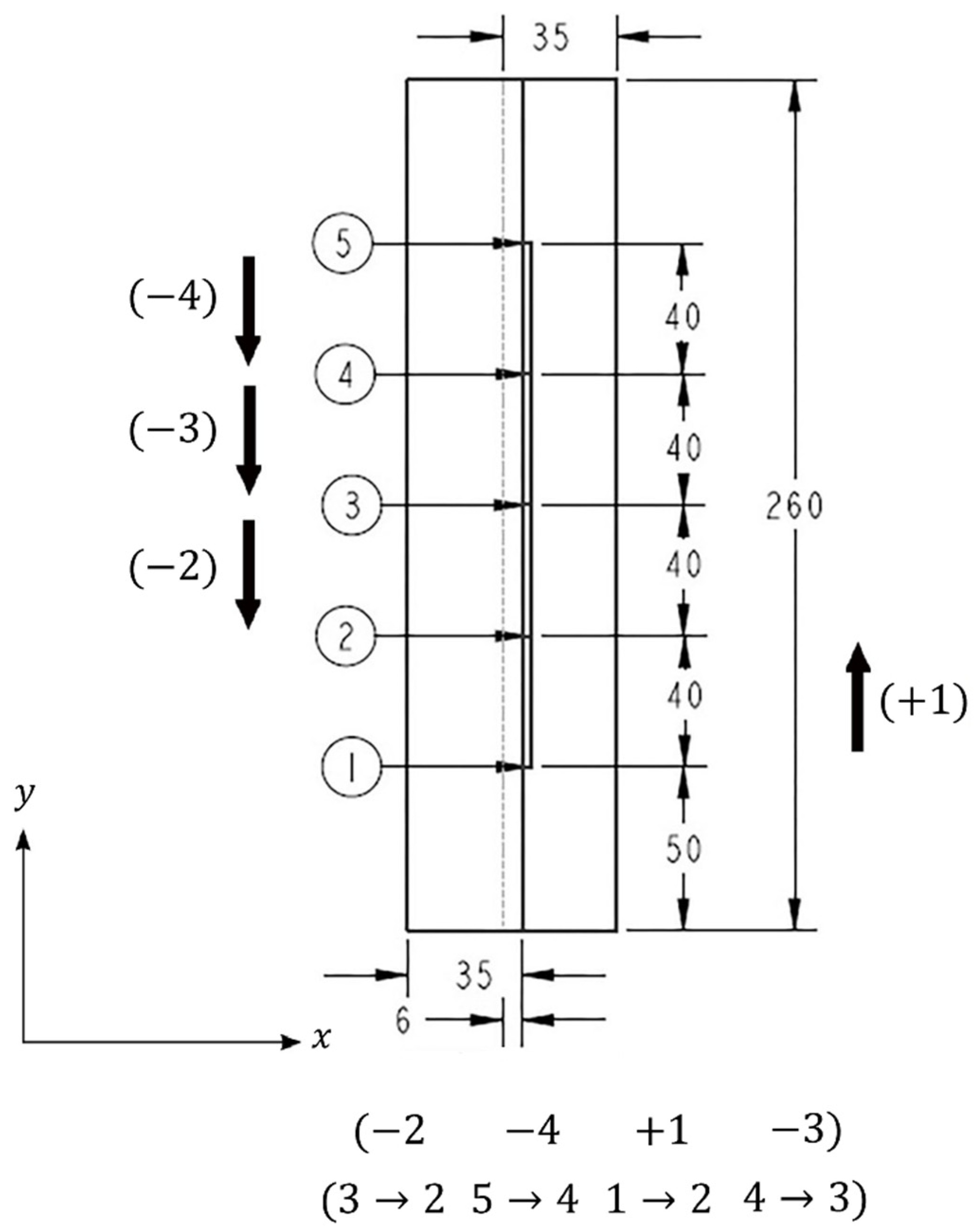
In the above equation, $C_{x1}$ is the x-coordinate of state 1, which is the current state, and $C_{x2}$ is the x-coordinate of the future state, which is selected based on a higher Q value in the exploitation phase. Similarly, $C_{y1}$ and $C_{y2}$ are the corresponding values of y-coordinates. Equation (3) gives a reward for 2D problems or weld segments lying on the same plane. For 3D problems, Equation (3) can be extended using z-coordinates for vectors in 3D space. The reward system proposed in this research reinforces the welding robots to adopt a skip welding sequence that has a balancing effect. If welding heat and shrinkage forces are produced in one corner of the welding assembly, the welding robot moves to the next opposite corner to counter the shrinkage force. The reward system enforces the robot to adopt this pattern. The optimum weld sequence obtained after 160 iterations is shown in Figure 12. This welding sequence is in line with the best welding practices used by welders to avoid distortion by using a back-step or skip welding. This technique is explained by Bill Lucas [26] in an article published by the UK welding society, TWI (The Welding Institute).

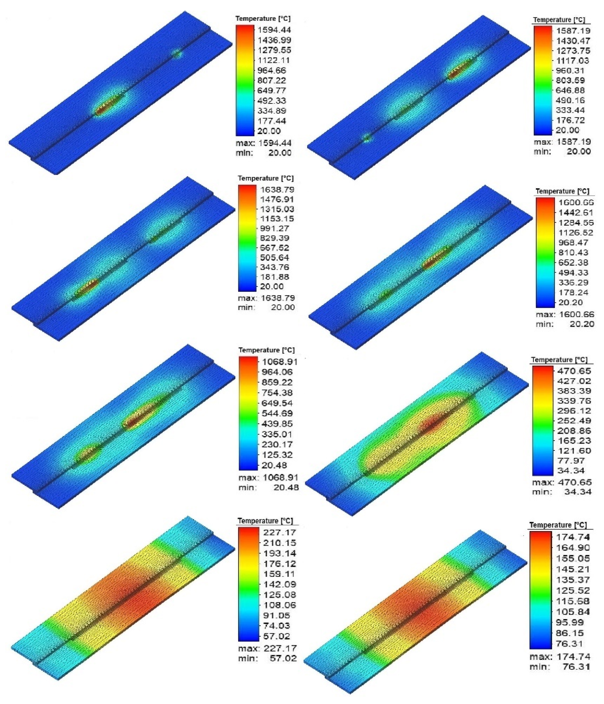
The optimum welding sequence could have been started with −1 + 4 with a maximum reward. In that case, the remaining weld segments (±2 and ±3) would be very close to each other and would result in heat accumulation in that region. The temperature map demonstrating temperature evolution during different phases of the weld sequence, including the cooling phase, is shown in Figure 13.

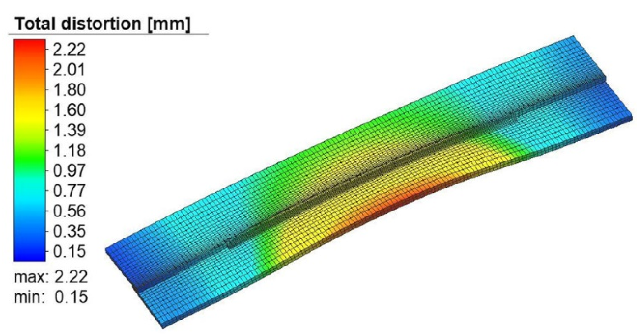
The welding simulation is performed by using the weld parameters mentioned in Table 2. These weld parameters were optimized during the response surface optimization study. Welding simulation is performed with optimum welding parameters and a random welding sequence. The maximum distortion observed is 2.2 mm, as shown in Figure 14. The optimum weld sequence is obtained by 115 iterations. The computational time for these iterations is less than a minute. The methodology proposed by Hdz et al. [10] involves welding simulation during MDP (Markovian Decision Process) to calculate the reward for each transition state. To run one iteration, a complete welding simulation is required.

The iteration number 1–50 in Figure 15 is the exploration phase. In this phase, a maximum reward of 284 is observed. From iteration number 50 onwards, a maximum reward of 324 is achieved. In this phase, the minimum reward is 200. The learning rate ‘α’ is 0.5 and the discount rate ‘γ’ used in this algorithm is 0.8. The distortion produced during the simulation of the optimum weld sequence is shown in Figure 16.

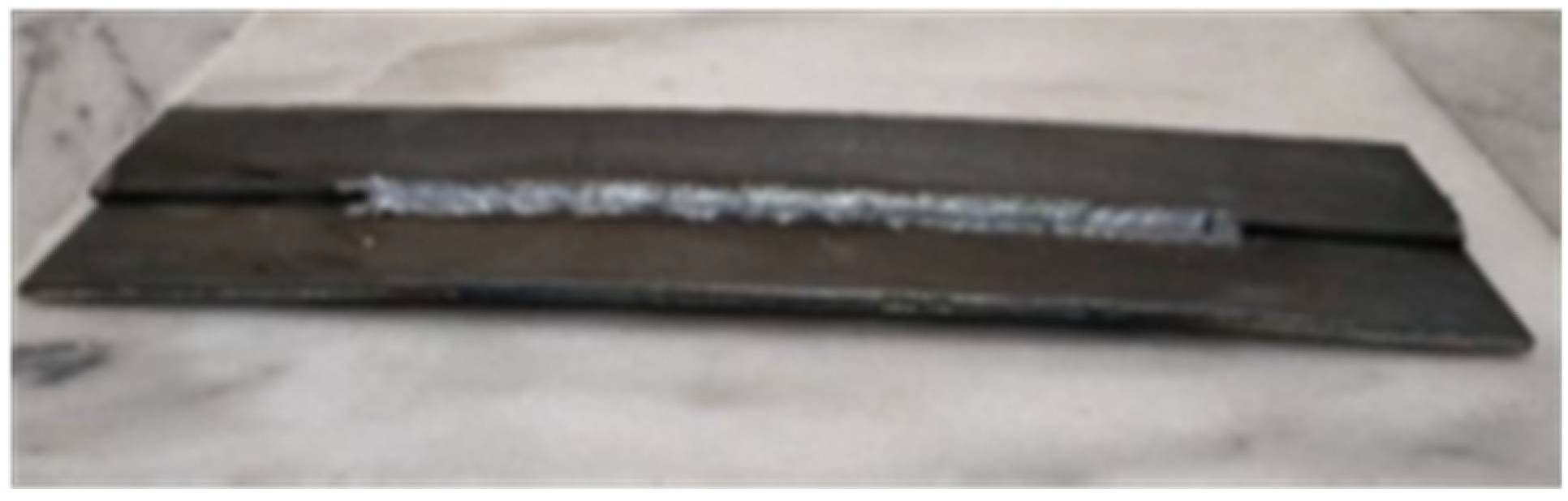
Finally, a test sample is prepared to validate the results of minimum distortion obtained under optimized weld parameters and weld sequence. The test sample is shown in Figure 17. In the test sample, welding distortion is measured along the edge of the bottom plate. The distortion values are plotted against the distance along the length of the plate, as shown in Figure 18. The results show agreement between the distortion values of the optimum weld simulation and the test sample.

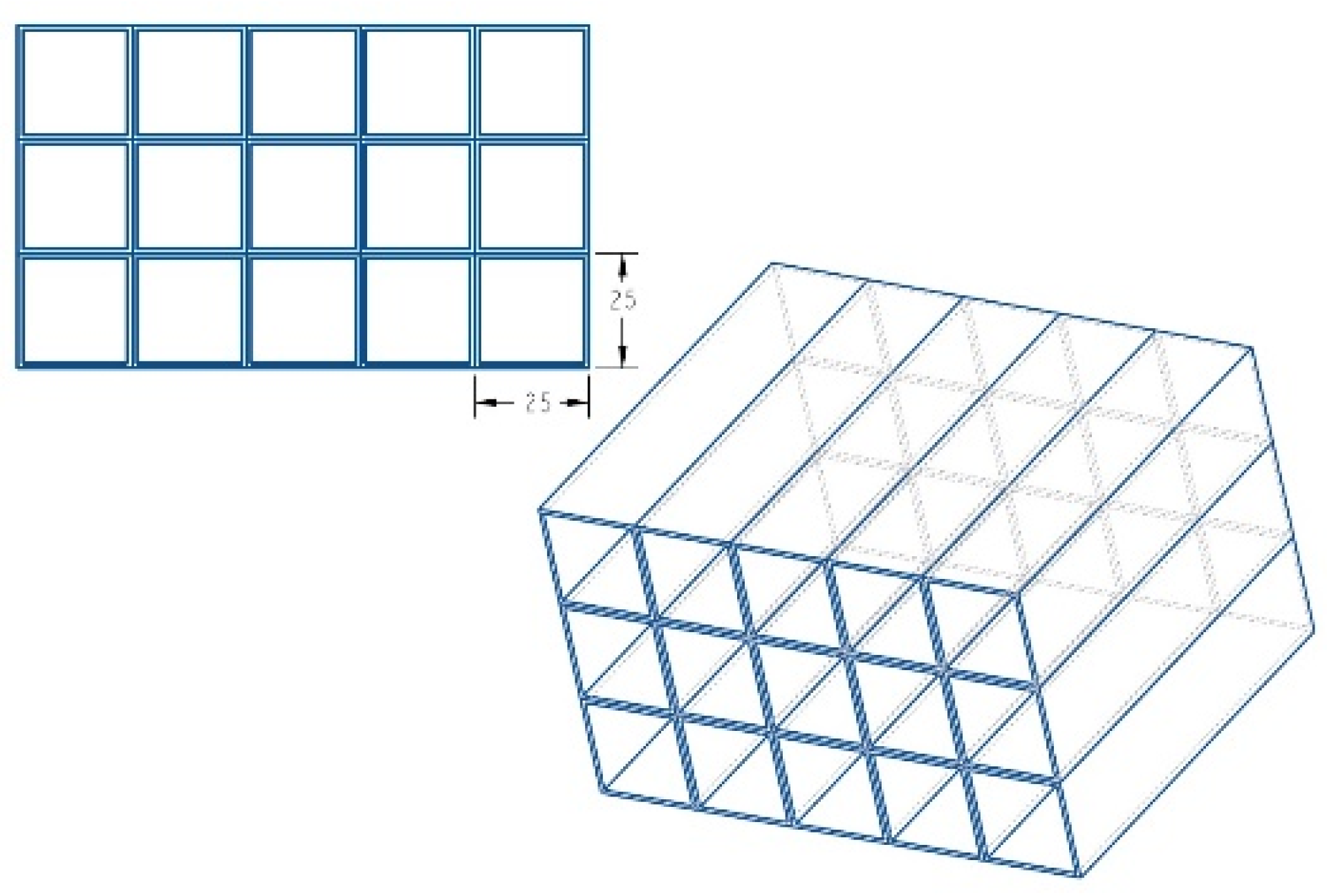
5.2. Vent Panel Case Study

Rectangular or square tube vent panels are used in air conditioning ducts, as flow straighteners, and for EMI (Electromagnetic Interference) shielding purposes. In this case study, a 15-cell vent panel is considered with square tubes of size 25 mm × 25 mm. The 15 tubes are cut to the length of 125 mm and joined together to form an airflow vent panel, as shown in Figure 19.

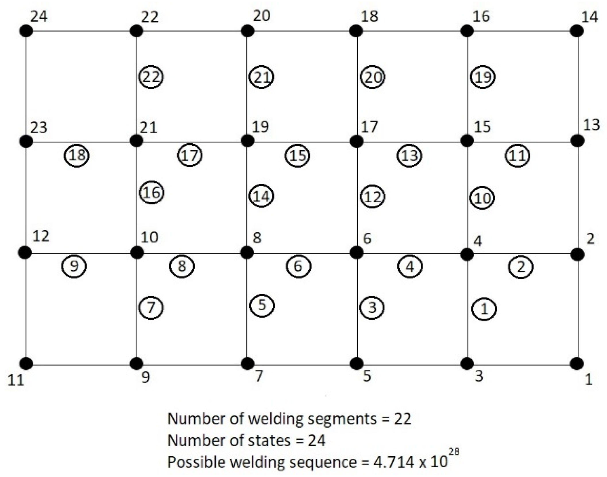
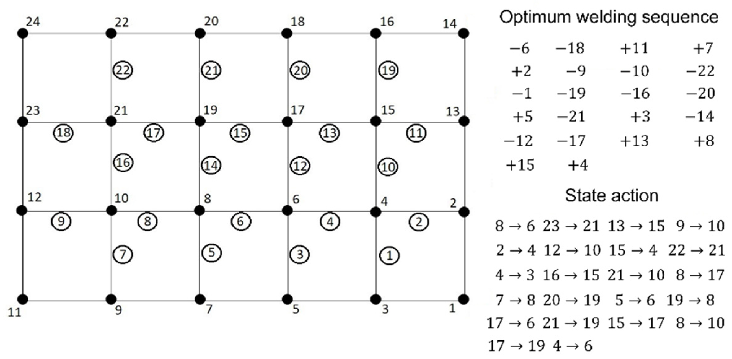
There are 22 weld segments that join the square tube sections to form the vent panel assembly. As discussed in the lap joint case study, all the weld segments can be welded in two directions. The total number of possible weld sequences and the number of states to be visited by a welding robot are given in Figure 20. States 1, 11, 14, and 24 are not utilized; they are used for numbering consistency. A total number of 44 actions are entered in the state action matrix. The coordinate of each state is stored in a separate matrix. The reinforcement learning algorithm mentioned in Section 5.1 is used to find an optimum welding sequence.

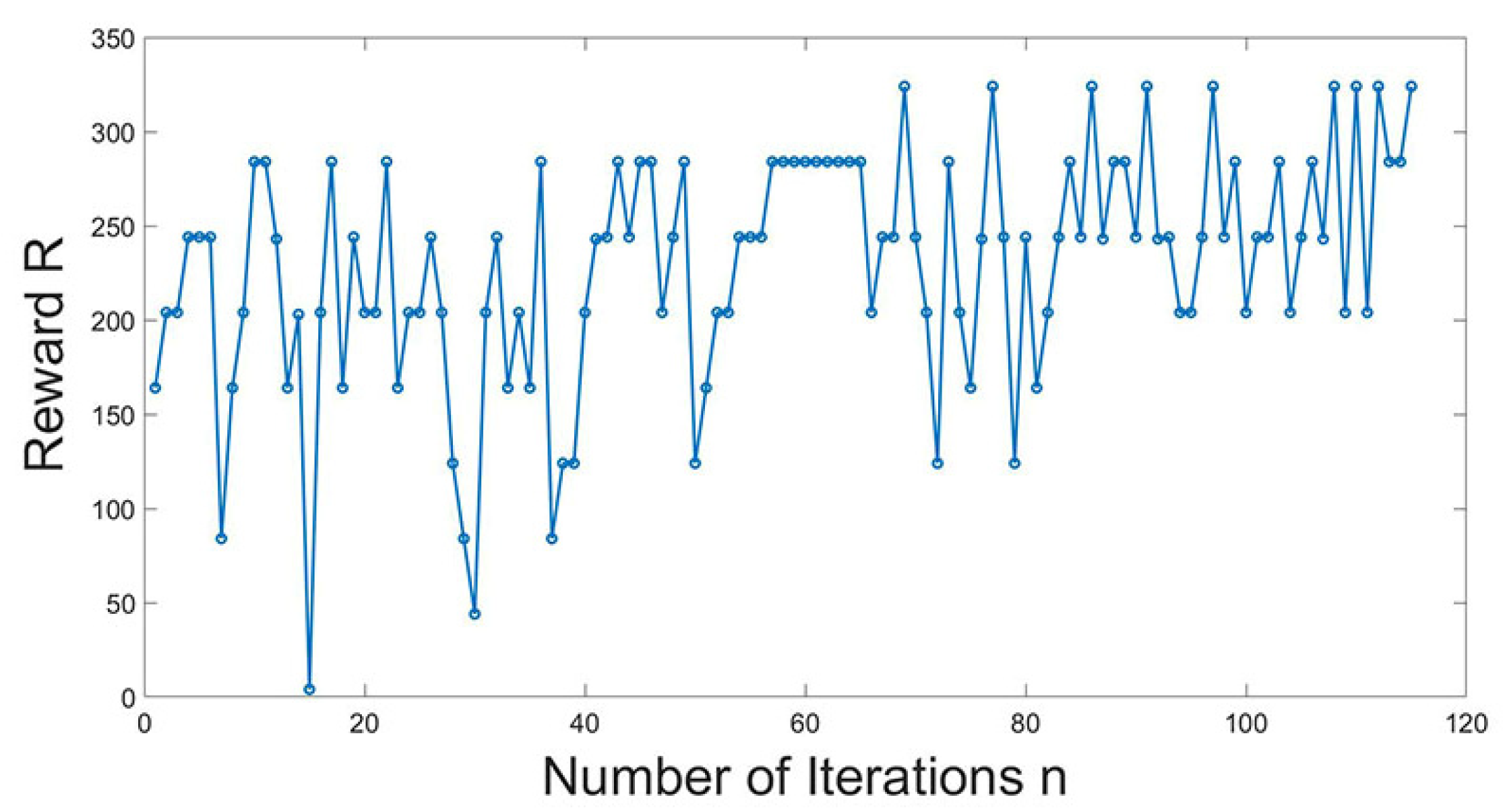
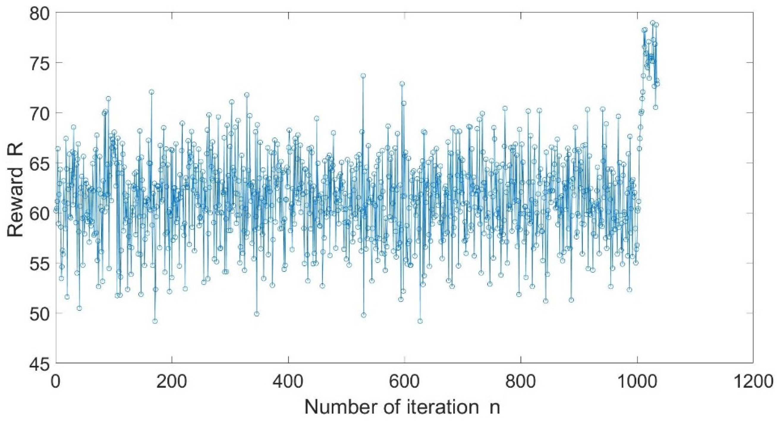
The number of initial iterations has been increased to 800. This is executed to expand the exploration phase and populate the Q matrix. To calculate the reward matrix, each dimension is divided by 25 mm. The reward is constrained in the range from 1 to 100 to manage the plotting of iteration number vs. reward. The plot for iteration number ‘n’ vs. reward ‘R’ is shown in Figure 21.

For the first 1000 iterations, the average reward is 62. The last 50 iterations have an average of 75. The maximum reward of 78.95 is observed at iteration number 112. The optimum sequence for this episode is given in Figure 22.

The sign convention used in the optimum sequence is ‘$+$’, or forward, for a lower number state to a higher number state, i.e., in the transition from state 2 to 4, $+$2 is used. Similarly, the transition from a higher number state to a lower number state is represented by a ‘−’ sign, or reverse direction. The direction and location of welds have a balancing effect, as discussed in the previous section. The welding segment pairs $+$2, $-$9 and $-$1, $-$19 are examples of such combinations. The optimum welding sequence is simulated to find minimum distortion.

The optimum weld parameters for the butt joint configuration are calculated by procedures mentioned in Section 4. The value for optimum weld parameters is given in

Table 3. Optimum weld parameters for vent panel.

Current	Voltage	Speed
70 A	11 V	4.5 mm/s

.

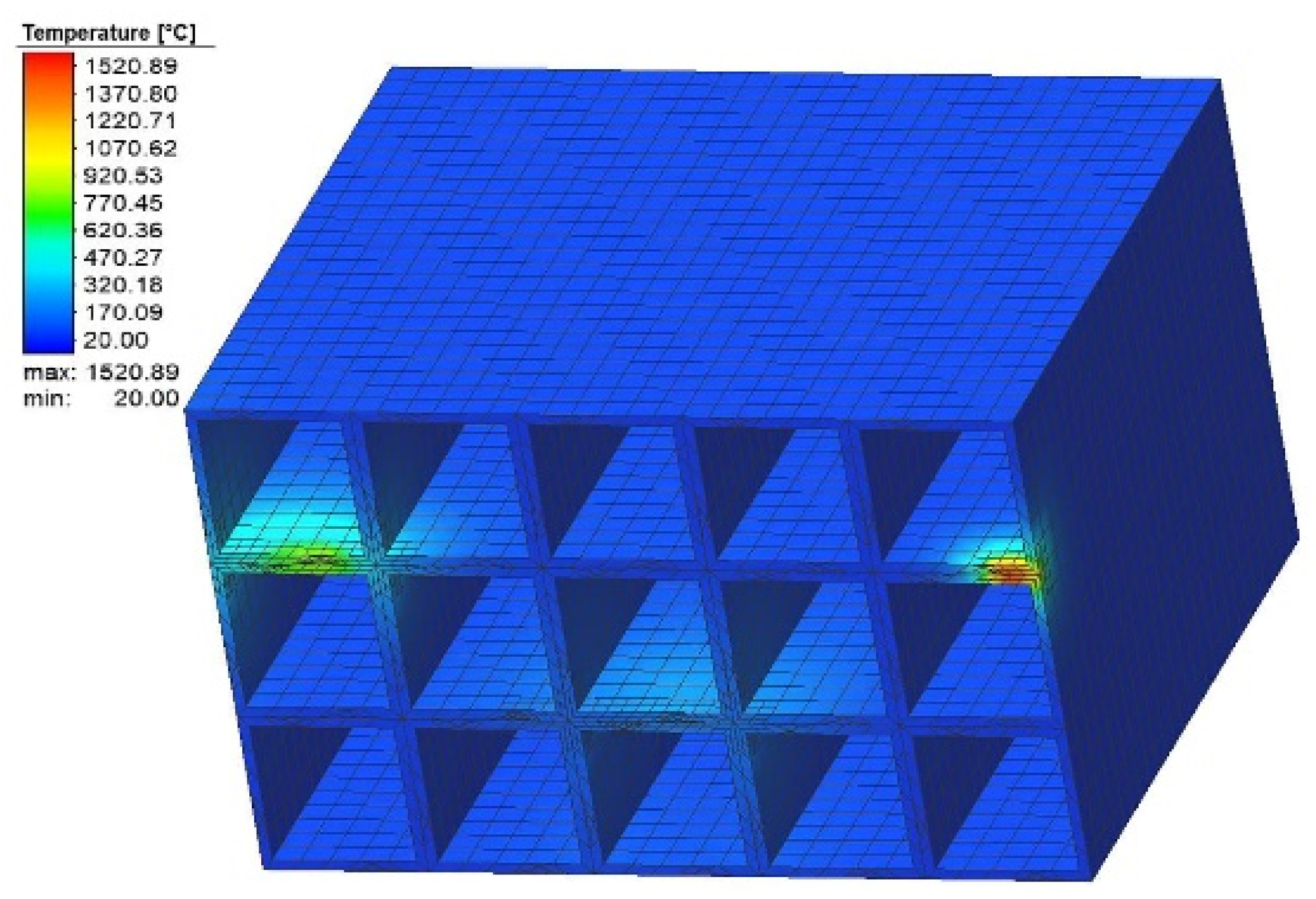
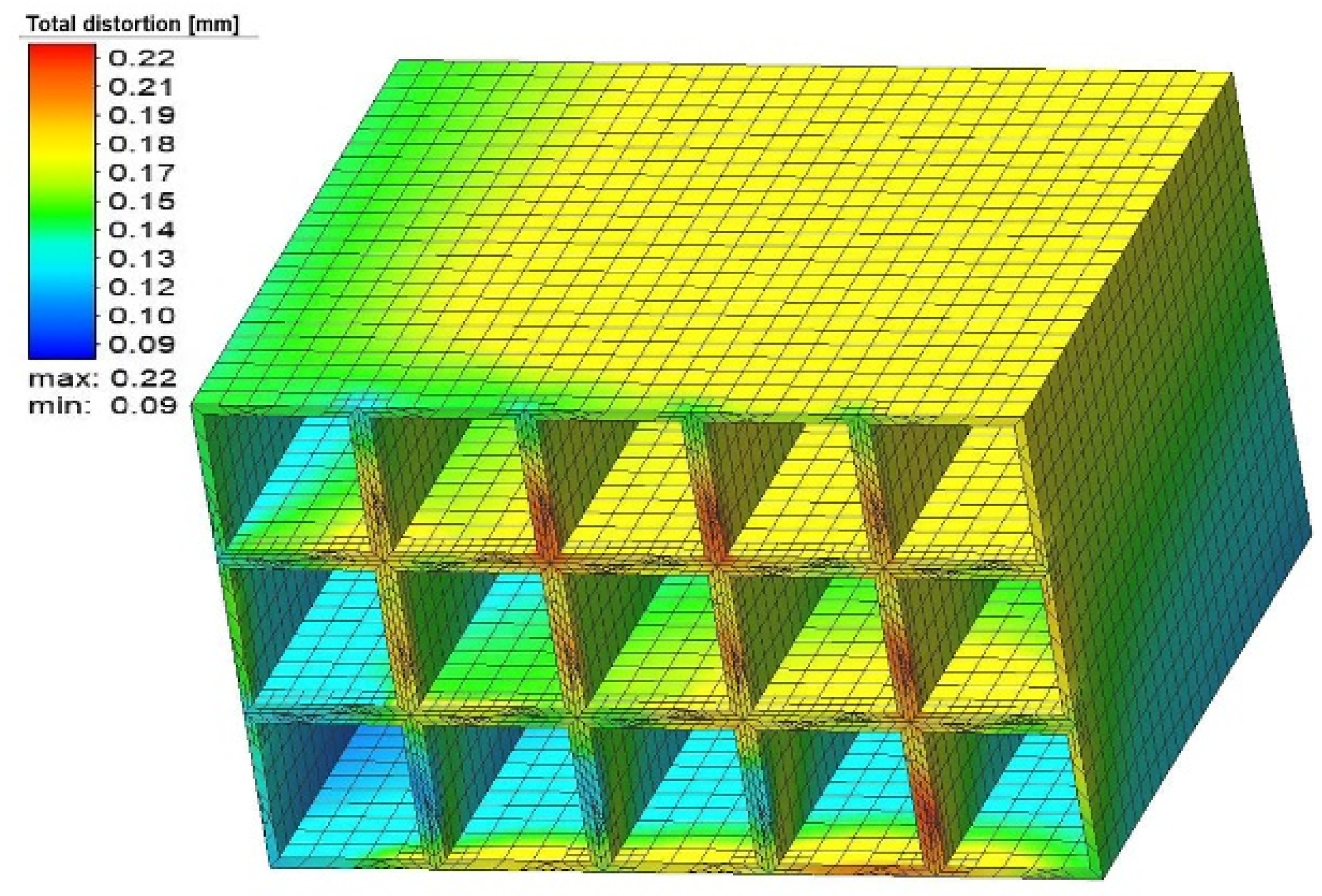
The temperature profile after the second weld segment is shown in Figure 23. The heat flux does not accumulate at any instant within the whole assembly to be welded. The distortion induced due to welding is shown in Figure 24. The value of maximum distortion is 0.22 mm.

6. Conclusions

In this research, an effort has been made to combine the weld parameter and weld sequence optimization in a framework. The output of this framework is minimum welding induced distortion for a given base material and joint configuration. The framework devised in this research gives a comprehensive approach for weld induced distortion mitigation at the design stage. The following tasks were performed.

• Weld simulations of 3 mm thick steel plates in a lap joint configuration were performed using finite element analysis. Three weld parameters i.e., welding current, voltage, and speed were selected for optimization through the design of experiment and response surface method. The optimum weld parameters were selected by studying contour plots obtained from the regression analysis.
• In the next phase, weld sequence optimization was performed using the optimum weld parameters. Q-learning based reinforcement learning was efficiently applied to find the optimum weld sequence.
• A comparison of the results revealed that minimum distortion is produced during weld simulations of an optimum weld sequence having optimum weld parameters. The combination of weld parameters and weld sequence optimization reduces the welding induced distortion by 19%. A test sample validates the simulated results.
• In a further case study, square tubes were welded together to form a vent panel assembly. The optimum weld parameters and weld sequence were found to predict minimum distortion in the structure.