Theoretical Analysis of Roll-Over-Web Surface Thin Layer Coating

Abstract

This study presents the theoretical investigation of a roll-over thin layer formation under the lubrication approximation theory. The set of differential equations derived by lubrication approximation is solved by the optimal homotopy asymptotic method (OHAM) to obtain precise expressions for pressure and velocity gradients. Critical quantities such as velocity, pressure gradient, and coating layer depth are numerically estimated. The impact of parameters affecting the coating and layer formation is revealed in detail. Results indicate that the transport properties of the higher-grade fluid play an essential role in regulating velocity, pressure, and the final coated region. Moreover, couple stress effects on the properties of fluid particles to be coated on roller-surface have also been studied.

1. Introduction

Roll-coating is a technique in which liquid is allowed to flow over a sheet/web to form a micro-nano scale thin layer coating over a surface. The main objective of the thin layer coating is to improve the quality, service life, and efficiency of the surface. As a result of its practical advantages and application, the coating is extensively used at the industrial level. It is mostly involved in various processes such as the production of paper, paperboard, cellulose thin films, plastic coatings, fibrous fabric sheets, metallic foils, etc. Most of the materials used during the roll-coating process are non-Newtonian fluids, which exhibit either viscoelastic or pseudoelastic behavior [1,2].

Greener and Middleman [3] conducted the theoretical analysis on roll-coating under the assumption of a small roll curvature and discussed the case when both roll and sheet are at the same speed. For a Newtonian fluid, they obtained the exact expression for film thickness and pressure distribution under the approximation of lubrication. For viscoelastic and power law fluids they also numerically computed film thickness, pressure, and roll-separating force. Coyle et al. [4] solved the complete Navier-Stokes equations by finite element method, compared the results of the approximation lubrication model, and observed that the lubrication model was accurate only for high capillary number with low surface tension. Hintermaier and White [5] studied the movement of water between the two rollers by adding a lubricating pattern, and their measured approaches were close to their experimental findings. Benkreira et al. [6,7,8,9] examined the coating flows for Newtonian and different non-Newtonian fluid models theoretically and experimentally. Sofou and Missoula [10] investigated the roll over-web coating flow numerically using the power lubrication theory, Bingham plastics, and Hershel–Bulkley models. Zahid et al. [11] investigated the roll coating process using a third-grade fluid lubrication approximation and numerically estimated all the important properties. Zahid et al. [12] also theoretically investigated the second grade fluid roll coating process by taking both the roller and sheet as porous. It is assumed that the rate of fluid entering the roller surface is equal to the rate of fluid leaving across the surface of the web. Ali et al. [13] studied the web-coating technique for a couple stress fluid by using the lubrication approximation theory. Moreover, they measured all the essential properties such as pressure gradient, pressure, velocity, roll-separating force, power input, and velocity. Compared the results with Newtonian fluid by reaching infinity to the couple stress parameter. Gaskell et al. [14] used an optical sectioning procedure to study both the forward and the reverse roll-coating process in meniscus fluid mechanics experimentally. A series of experiments were conducted to calculate essential properties such as inlet flow rate, film thickness, meniscus location, and pressure field. However, no attempt was made to measure the effects of couple stresses initiated during the roll-over-web process through the optimal homotopy asymptotic method (OHAM).

Optimal homotopy asymptotic method is a semi-analytical approximate approach to solve non-linear problems [15,16,17,18,19,20]. This technique is independent of any large/small parameters as compared to other method of perturbation. This technique provides an appropriate approach to control the approximation solution convergence and adjust the convergence regions when necessary. In this study, OHAM is proposed and has been applied to roll-over-web process for high-grade fluid (HGF) flow. The model of roll-web coating is taken from [12,21,22,23]. This manuscript is categorized in four sections. In Section 1; the governing equation based upon roller-web approach is formulated. In Section 2; computational remarks for solution based on OHAM are given. The results are discussed in Section 3, narrating some cases as examples. Finally, whole work is summarized.

2. Materials and Methods

Consider a coating on a sheet of fluid with stress which is couple in state operation with isothermal steady as shown in Figure 1. The radius of roll in cylindrical is $R^{*}$, with its anti-clockwise rotation and with angular velocity ${\omega }^{*}$. $U_2^{*}={\omega }^{*}{R}^{*}$ is its linear velocity. The movement of plate considered is with uniform velocity $U_1^{*}$ and in the direction of positive x-axis $H_0$ is the width called as nip-region between plate and roll. The melt polymer first bites the plane at $x^{*}={\eta }_b^{*}$ is the position where melted polymer crosses the plane. For the consideration of flow in either sides in the parallel boundaries and the nip region, the assumption $\frac{H_0}{R^{*}}\ll 11$ is made [1,13]. The above assumptions assure the validity of theory of lubrication in nearby nip region.

For the velocity field in two-dimensions $[u^{*}(x^{*},y^{*}),{\nu }^{*}(x^{*},y^{*}),0]$, the equations depicting the flow of couple stress fluid which is incompressible, without taking into account the presence of body force are given by [1,13]

$$\begin{array}{c}\frac{\partial u^{*}}{\partial x^{*}}=-\frac{\partial {\nu }^{*}}{\partial y^{*}}\end{array}$$

(1)

$$\begin{array}{c}\hfill \rho \left[u^{*}\frac{\partial u^{*}}{\partial x^{*}}+{\nu }^{*}\frac{\partial u^{*}}{\partial y^{*}}\right]+\frac{\partial p^{*}}{\partial x^{*}}+\eta \left(\frac{{\partial }^4{u}^{*}}{\partial x^{*4}}+\frac{{\partial }^4{u}^{*}}{\partial y^{*4}}\right)=\mu \left(\frac{{\partial }^2{u}^{*}}{\partial x^{*2}}+\frac{{\partial }^2{u}^{*}}{\partial y^{*2}}\right)\end{array}$$

(2)

$$\begin{array}{c}\hfill \rho \left[u^{*}\frac{\partial {\nu }^{*}}{\partial x^{*}}+{\nu }^{*}\frac{\partial {\nu }^{*}}{\partial y^{*}}\right]+\frac{\partial p^{*}}{\partial y^{*}}+\eta \left(\frac{{\partial }^4{\nu }^{*}}{\partial x^{*4}}+\frac{{\partial }^4{\nu }^{*}}{\partial y^{*4}}\right)=\mu \left(\frac{{\partial }^2{\nu }^{*}}{\partial x^{*2}}+\frac{{\partial }^2{\nu }^{*}}{\partial y^{*2}}\right)\end{array}$$

(3)

with the appropriate boundary conditions

$$\begin{array}{c}{u}^{*}(x^{*},0)=U_1^{*}\hfill \end{array}$$

(4)

$$\begin{array}{c}{u}^{*}(x^{*},h^{*}\left(x^{*}\right))=U_2^{*}\hfill \end{array}$$

(5)

where $\rho ,p^{*},\mu$ and $\eta$ represent the density, pressure, viscosity and momentum constant respectively. Due to the requirement that at roll and sheet surfaces the couple stress must vanish, also microelement rotational motion is absent near solid boundaries, the two more conditions are as follows [1,13]:

$$\begin{array}{cc}& \frac{{\partial }^2{u}^{*}}{\partial y^{*2}}(x^{*},0)=0\hfill \end{array}$$

(6)

$$\begin{array}{cc}& \frac{{\partial }^2{u}^{*}}{\partial y^{*2}}(x^{*},h^{*}\left(x^{*}\right))=0\hfill \end{array}$$

(7)

Here from the sheet, roll height is denoted by $h^{*}\left(x^{*}\right)$

$$\begin{array}{c}\hfill h^{*}\left(x^{*}\right)=\frac{x^{*2}}{2R^{*}}+H_0\end{array}$$

(8)

With the scales for $x^{*},y^{*}$ and ${\mathrm{u}}^{*}$

$$\begin{array}{c}\hfill x^{*}\sim L_c^{*},u^{*}\sim U_1^{*},y^{*}\sim H_0\end{array}$$

(9)

For velocity and pressure, their characteristic scales are [1,13]

$$\begin{array}{cc}& L_c^{*}=\sqrt{2R^{*}{H}_0}\hfill \end{array}$$

(10)

$$\begin{array}{cc}& p^{*}\sim \sqrt{\frac{2R^{*}}{H_0}}\frac{\mu U_1^{*}}{H_0}\hfill \end{array}$$

(11)

Defining the non−dimensional variables as follows [1,13]:

$$\begin{array}{cc}& x=\frac{x^{*}}{\sqrt{2R^{*}{H}_0}},y=\frac{y^{*}}{H_0},h\left(x\right)=\frac{h^{*}\left(x^{*}\right)}{H_0},u=\frac{u^{*}}{U_1^{*}},\nu =\sqrt{\frac{2R^{*}}{H_0}}\frac{{\nu }^{*}}{U_1^{*}},\hfill \\ & p=\sqrt{\frac{H_0}{2R^{*}}}\frac{H_0}{\mu U_1^{*}}{p}^{*},\gamma =\frac{H_0}{l}\hfill \end{array}$$

(12)

With these variables, the Equations (1)–(3) become

$$\begin{array}{c}\hfill \frac{\partial u}{\partial x}=-\frac{\partial \nu }{\partial y}\end{array}$$

(13)

$$\begin{array}{c}\hfill \mathrm{Re}B\left[u\frac{\partial u}{\partial x}+\nu \frac{\partial u}{\partial y}\right]+\frac{\partial p}{\partial x}+\frac{1}{y^2}\left(B^2\frac{{\partial }^{4}u}{\partial x^4}+\frac{{\partial }^{4}u}{\partial y^4}\right)=B^2\frac{{\partial }^{2}u}{\partial x^2}+\frac{{\partial }^{2}u}{\partial y^2}\end{array}$$

(14)

$$\begin{array}{c}\hfill \mathrm{Re}{B}^3\left[u\frac{\partial \nu }{\partial x}+\nu \frac{\partial \nu }{\partial y}\right]+\frac{\partial p}{\partial y}+\frac{B^4}{{\gamma }^2}\left(B^4\frac{{\partial }^4\nu }{\partial x^4}+\frac{{\partial }^4\nu }{\partial y^4}\right)=B^2\left(B^2\frac{{\partial }^2\nu }{\partial x^2}+\frac{{\partial }^2\nu }{\partial y^2}\right)\end{array}$$

(15)

In the above equations, $\mathrm{Re}=\frac{\rho U_1^{*}{H}_0}{\mu }$ is Reynolds value, $B={\left(H_0/2R^{*}\right)}^{1/2}<<1$ is dimensionless entity, $\gamma =H_0/l$ is the dimensionless couple stress parameter and $l=\sqrt{\eta /\mu }$ is the material constant.

Main velocity component $\mathrm{u}$ and pressure gradient $dp/dx$ are determined in further analysis and normal velocity component $\nu$ is not involved but can be computed using Equation (13) with known value of u [1,13].

Here geometric parameter $B={\left(H_0/2R^{*}\right)}^{1/2}<<1$, from Equations (14)) and (15))

$$\begin{array}{cc}& 0=-\frac{\partial p}{\partial x}+\frac{{\partial }^{2}u}{\partial y^2}-\frac{1}{{\gamma }^2}\frac{{\partial }^{4}u}{\partial y^4}\hfill \end{array}$$

(16)

$$\begin{array}{cc}& 0=-\frac{\partial p}{\partial y}\hfill \end{array}$$

(17)

From Equation (17), it follows

$$\begin{array}{c}\hfill \frac{{\partial }^{2}u}{\partial y^2}-\frac{1}{{\gamma }^2}\frac{{\partial }^{4}u}{\partial y^4}=P\end{array}$$

(18)

where $P=\frac{dp}{dx}$, and with

$$\begin{array}{c}\hfill u\left(0\right)=1,u(1+\frac{x^2}{2})=U,\frac{{\partial }^{2}u}{\partial y^2}\left(0\right)=0,\frac{{\partial }^{2}u}{\partial y^2}(1+\frac{x^2}{2})=0\end{array}$$

(19)

Assume that $U=1$ is the same speed of sheet and roll. The condition for faster speed of roll than web is $U>1$. In addition, $U<1$ is the condition for above reverse case.

3. Results

In this section, we will apply the Optimal Homotopy Analysis Method to nonlinear ordinary differential Equation (18). According to the OHAM, we can construct homotopy of Equation (18) as follows:

$$\begin{array}{c}\hfill (1-q)\left\{\frac{1}{{\gamma }^2}\frac{d^{4}u}{d{y}^4}+P\right\}-\left(C_{1}q+C_2{q}^2+C_3{q}^3\right)\left\{\frac{1}{{\gamma }^2}\frac{d^{4}u}{d{y}^4}-\frac{d^{2}u}{d{y}^2}+P\right\}=0\end{array}$$

(20)

We consider u as follows:

$$\begin{array}{c}\hfill u=u_0\left(\eta \right)+q{u}_1\left(\eta \right)+q^2{u}_2\left(\eta \right)\end{array}$$

(21)

Substituting value of u from (26) into (20), and some simplifications and rearranging based on powers of q-terms, we have

$$\begin{array}{cc}{\mathbf{q}}^{\mathbf{0}}:& \frac{1}{{\gamma }^2}\frac{d^4{u}_0}{d{y}^4}+P=0\hfill \end{array}$$

(22)

$$\begin{array}{cc}{\mathbf{q}}^{\mathbf{1}}:& -P-P{C}_1+C_1\frac{d^2{u}_0}{d{y}^2}-\frac{1}{{\gamma }^2}\frac{d^4{u}_0}{d{y}^4}-C_1\frac{1}{{\gamma }^2}\frac{d^4{u}_0}{d{y}^4}+\frac{1}{{\gamma }^2}\frac{d^4{u}_1}{d{y}^4}=0\hfill \end{array}$$

(23)

$$\begin{array}{cc}{\mathbf{q}}^{\mathbf{2}}:& -P{C}_2+C_2\frac{d^2{u}_0}{d{y}^2}+C_1\frac{d^2{u}_1}{d{y}^2}-C_2\frac{1}{{\gamma }^2}\frac{d^4{u}_0}{d{y}^4}-\frac{1}{{\gamma }^2}\frac{d^4{u}_1}{d{y}^4}-C_1\frac{1}{{\gamma }^2}\frac{d^4{u}_1}{d{y}^4}\hfill \\ & +\frac{1}{{\gamma }^2}\frac{d^4{u}_2}{d{y}^4}=0\hfill \end{array}$$

(24)

$$\begin{array}{cc}{\mathbf{q}}^{\mathbf{3}}:& -P{C}_3+C_3\frac{d^2{u}_0}{d{y}^2}+C_2\frac{d^2{u}_1}{d{y}^2}+C_1\frac{d^2{u}_2}{d{y}^2}-C_3\frac{1}{{\gamma }^2}\frac{d^4{u}_0}{d{y}^4}+C_2\frac{1}{{\gamma }^2}\frac{d^4{u}_1}{d{y}^4}\hfill \\ & -\frac{1}{{\gamma }^2}\frac{d^4{u}_2}{d{y}^4}-C_1\frac{1}{{\gamma }^2}\frac{d^4{u}_2}{d{y}^4}+\frac{1}{{\gamma }^2}\frac{d^4{u}_3}{d{y}^4}=0\hfill \end{array}$$

(25)

With the conditions from Equation (19)

$$\begin{array}{c}\hfill u_0\left(0\right)=1,u_0(1+\frac{x^2}{2})=U{u}_0^{″}\left(0\right)=0,u_0^{″}(1+\frac{x^2}{2})=0\end{array}$$

we get from Equation (22)

$$\begin{array}{cc}{u}_0\left(y\right)=& -\frac{1}{192\left(x^2+2\right)}\{{\gamma }^{2}P{x}^{8}y+8{\gamma }^{2}P{x}^{6}y-8P{x}^{4}y{\gamma }^2\left(y^2-3\right)\hfill \\ & +8x^2\left({\gamma }^{2}Py\left(y^3-4y^2+4\right)-24\right)+16({\gamma }^{2}P{y}^4-2{\gamma }^{2}P{y}^3-24\hfill \\ & +y\left({\gamma }^{2}P-24U+24\right)\left)\right\}\hfill \end{array}$$

and similarly with the conditions

$$\begin{array}{c}\hfill u_1\left(0\right)=0,u_1(1+\frac{x^2}{2})=0,u_1^{″}\left(0\right)=0,u_1^{″}(1+\frac{x^2}{2})=0\end{array}$$

we get $u_1\left(y\right)$ from Equation (23)

$$\begin{array}{cc}{u}_1\left(\eta \right)=& \frac{1}{23040}+Py\{-3x^{10}-30x^8+20x^6\left(y^2-6\right)+120x^4\left(y^2-2\right)\hfill \\ & -48x^2\left(5-5y^2+y^4\right)+32\left(-3+5y^2-3y^4+y^5\right)\}{\gamma }^4{C}_1.\hfill \end{array}$$

Now for $u_2\left(y\right)$, with the conditions

$$\begin{array}{cc}& u_2\left(0\right)=0,u_2(1+\frac{x^2}{2})=0,u_2^{″}\left(0\right)=0,u_2^{″}(1+\frac{x^2}{2})=0,u_2^{\prime \prime }\left(0\right)=0\hfill \\ & u_2^{″}(1+\frac{x^2}{2})=0\hfill \end{array}$$

we get $u_2\left(y\right)$ from Equation (24)

$$\begin{array}{cc}{u}_2\left(\eta \right)=& -\frac{{\gamma }^{4}Py}{5160960}\left[224\right\{3x^{10}+30x^8-20x^6\left(y^2-6\right)-120x^4\left(y^2-2\right)\hfill \\ & +48x^2\left(y^4-5y^2+5\right)-32\left(y^5-3y^4+5y^2-3\right)\left\}{C}_1\right\{17{\gamma }^2{x}^{14}\hfill \\ & +238{\gamma }^2{x}^{12}-28x^{10}\left({\gamma }^2(4y^2-51-24\right)-280x^8({\gamma }^2(4y^2-17)\hfill \\ & -24)+112x^6\left(85{\gamma }^2+2{\gamma }^2{y}^4-40({\gamma }^2+1)y^2+240\right)+224x^4(51{\gamma }^2\hfill \\ & +6{\gamma }^2{y}^4-40({\gamma }^2+3)y^2+240)+128(17{\gamma }^2+{\gamma }^2{y}^7-4{\gamma }^2{y}^6-56y^5\hfill \\ & +14({\gamma }^2+12)y^4-28({\gamma }^2+10)y^2+168)-64x^2(-7(17{\gamma }^2+120)\hfill \\ & +4{\gamma }^2{y}^6-42({\gamma }^2+4)y^4+140({\gamma }^2+6)y^2\left)\right\}{C}_1^2+224(3x^{10}+30x^8\hfill \\ & -20x^6(y^2-6)-120x^4(y^2-2)+48x^2(y^4-5y^2+5)-32(y^5-3y^4\hfill \\ & +5y^2-3\left)\right)C_2]\hfill \end{array}$$

Now, substituting the values in Equation (26), it gives

$$\begin{array}{cc}u\left(y\right)=& \frac{1}{5160960}[-\frac{1}{x^2+2}26880\{16(y({\gamma }^{2}P-24U+24)+{\gamma }^{2}P{y}^4-2{\gamma }^{2}P{y}^3\hfill \\ & -24)+{\gamma }^{2}P{x}^{8}y+8{\gamma }^{2}P{x}^{6}y-8{\gamma }^{2}P{x}^{4}y(y^2-3)+8x^2({\gamma }^{2}Py(y^3-4y^2\hfill \\ & +4)-24)\}+224Py\{-3x^{10}-30x^8+20x^6(y^2-6)+120x^4(y^2-2)\hfill \\ & -48x^2(y^4-5y^2+5)+32(y^5-3y^4+5y^2-3)\}{\gamma }^4{C}_1-{\gamma }^{4}Py\{224(3x^{10}\hfill \\ & +30x^8-20x^6(y^2-6)-120x^4(y^2-2)+48x^2(y^4-5y^2+5)-32(y^5-3y^4\hfill \\ & +5y^2-3\left)\right)C_1+[17{\gamma }^2{x}^{14}+238{\gamma }^2{x}^{12}-28x^{10}\left({\gamma }^2(4y^2-51)-24\right)\hfill \\ & -280x^8\left({\gamma }^2(4y^2-17)-24\right)+112x^6(85{\gamma }^2+2{\gamma }^2{y}^4-40({\gamma }^2+1)y^2\hfill \\ & +240)+224x^4\left(51{\gamma }^2+6{\gamma }^2{y}^4-40({\gamma }^2+3)y^2+240\right)-64x^2(-7(17{\gamma }^2\hfill \\ & +120)+4{\gamma }^2{y}^6-42({\gamma }^2+4)y^4+140({\gamma }^2+6)y^2)+128(17{\gamma }^2+{\gamma }^2{y}^7\hfill \\ & -4{\gamma }^2{y}^6-56y^5+14({\gamma }^2+12)y^4-28({\gamma }^2+10)y^2+168\left)\right]C_1^2+224(3x^{10}\hfill \\ & +30x^8-20x^6(y^2-6)-120x^4(y^2-2)+48x^2(y^4-5y^2+5)-32(y^5-3y^4\hfill \\ & +5y^2-3\left)\right)C_2\left\}\right]\hfill \end{array}$$

(26)

Now finding the constants $C_1$ and $C_2$, we apply method of least squares as in [15,16,17,18]. With the choice of $P=-0.5;x=0;U=1.$ and with different values of $\gamma$, the values of constants are calculated as shown in the

Table 1. Values of $\gamma$, $C_1$ and $C_2$.

$\mathit{P}=-0.5;\mathit{x}=0;\mathit{U}=1.$
$\mathbf{\gamma }$	${\mathit{C}}_1$	${\mathit{C}}_2$
2	$-0.7117859161990184$	$0.22998908723027278$
3	$-0.5231969223195763$	$0.36317986919894485$
4	$-0.3816089014437683$	$0.4631762625722552$
5	$-0.2830976700342593$	$0.5327497179167221$

.

Corresponding to these values of constants as in Table 1, the values of $u\left(y\right)$ are calculated as shown in the Equations (27)–(30).

$$\begin{array}{cc}{u}_{(\gamma =2)}=& 0.000402095y^8-0.00160838y^7+0.00763271y^6-0.0172688y^5\hfill \\ & +0.0833333y^4-0.139762y^3+0.0672708y+1\hfill \end{array}$$

(27)

$$\begin{array}{cc}{u}_{(\gamma =3)}=& 0.00247461y^8-0.00989845y^7+0.0230332y^6-0.034455y^5\hfill \\ & +0.1875y^4-0.329123y^3+0.160469y+1\hfill \end{array}$$

(28)

$$\begin{array}{cc}{u}_{(\gamma =4)}=& 0.00739684y^8-0.0295874y^7+0.0274518y^6+0.0212005y^5\hfill \\ & +0.333333y^4-0.736519y^3+0.376724y+1\hfill \end{array}$$

(29)

$$\begin{array}{cc}{u}_{(\gamma =5)}=& 0.015529y^8-0.0621158y^7-0.0202685y^6+0.278211y^5\hfill \\ & +0.520833y^4-1.57782y^3+0.845631y+1\hfill \end{array}$$

(30)

Now with the choice of $P=0.5;x=0;U=1.$ and with different values of $\gamma$, the values of constants are calculated as shown in the

Table 2. Values of $\gamma$, $C_1$ and $C_2$.

$\mathit{P}=0.5;\mathit{x}=0;\mathit{U}=1.$
$\mathbf{\gamma }$	${\mathit{C}}_1$	${\mathit{C}}_2$
2	$-0.7117859161990184$	$0.22998908723027278$
3	$-0.5231969223195763$	$0.36317986919894485$
4	$-0.3816089014437683$	$0.4631762625722552$
5	$-0.2830976700342593$	$0.5327497179167221$

.

Corresponding to these values of constants as in Table 2, the values of $u\left(y\right)$ are calculated as shown in the Equations (31)–(34).

$$\begin{array}{cc}{u}_{(\gamma =2,P=0.5)}=& -0.000402095y^8+0.00160838y^7-0.00763271y^6+0.0172688y^5\hfill \\ & -0.0833333y^4+0.139762y^3-0.0672708y+1\hfill \end{array}$$

(31)

$$\begin{array}{cc}{u}_{(\gamma =3,P=0.5)}=& -0.00247461y^8+0.00989845y^7-0.0230332y^6+0.034455y^5\hfill \\ & -0.1875y^4+0.329123y^3-0.160469y+1\hfill \end{array}$$

(32)

$$\begin{array}{cc}{u}_{(\gamma =4,P=0.5)}=& -0.00739684y^8+0.0295874y^7-0.0274518y^6-0.0212005y^5\hfill \\ & -0.333333y^4+0.736519y^3-0.376724y+1\hfill \end{array}$$

(33)

$$\begin{array}{cc}{u}_{(\gamma =5,P=0.5)}=& -0.015529y^8+0.0621158y^7+0.0202685y^6-0.278211y^5\hfill \\ & -0.520833y^4+1.57782y^3-0.845631y+1\hfill \end{array}$$

(34)

Now with the choice of $P=0.5;x=1;U=1.$ and with different values of $\gamma$, the values of constants are calculated as shown in the

Table 3. Values of $\gamma$, $C_1$ and $C_2$.

$\mathit{P}=0.5;\mathit{x}=0;\mathit{U}=1.$
$\mathbf{\gamma }$	${\mathit{C}}_1$	${\mathit{C}}_2$
2	$-0.5231969223195738$	$0.36317986919894657$
3	$-0.32775265538407$	$0.5012121806766487$
4	$-0.21519795933137797$	$0.5807038184075737$
5	$-0.1492838624605476$	$0.6272555811822184$

.

Corresponding to these values of constants as in Table 3, the values of $u\left(y\right)$ are calculated as shown in the Equations (35)–(38).

$$\begin{array}{cc}{u}_{(\gamma =2,x=1)}=& -0.00021725y^8+0.0013035y^7-0.00454977y^6+0.0102089y^5\hfill \\ & -0.0833333y^4+0.219415y^3-0.240703y+1.\hfill \end{array}$$

(35)

$$\begin{array}{cc}{u}_{(\gamma =3,x=1)}=& -0.000971112y^8+0.00582667y^7-0.00263651y^6-0.0340208y^5\hfill \\ & -0.1875y^4+0.724492y^3-0.85482y+1\hfill \end{array}$$

(36)

$$\begin{array}{cc}{u}_{(\gamma =4,x=1)}=& -0.00235226y^8+0.0141136y^7+0.0349543y^6-0.268439y^5\hfill \\ & -0.333333y^4+2.09y^3-2.60454y+1\hfill \end{array}$$

(37)

$$\begin{array}{cc}{u}_{(\gamma =5,x=1)}=& -0.00431813y^8+0.0259088y^7+0.152332y^6-0.889527y^5\hfill \\ & -0.520833y^4+5.05125y^3-6.48238y+1\hfill \end{array}$$

(38)

Now for determining the pressure, we have by [1]

$$\begin{array}{c}\hfill \lambda ={\int }_0^{\frac{x^2}{2}+1}udy\end{array}$$

(39)

After substitution the expression of $\mathrm{u}$ from Equation (26) into (39), gives

$$\begin{array}{cc}\lambda =& -\frac{1}{185794560\left(x^2+2\right)}\left\{{\gamma }^{4}P{(x^2+2)}^8\right[C_1\{C_1\left(31{\gamma }^2{(x^2+2)}^2+1224\right)\hfill \\ & +2448\}+1224C_2]+48384{(x^2+2)}^2\left({\gamma }^{2}P{(x^2+2)}^4-960(U+1)\right)\}\hfill \end{array}$$

which implies

$$\begin{array}{c}\hfill \frac{dP}{dx}=\frac{(1/4)(1+U)(2+x^2)-\lambda }{Denominator}\end{array}$$

where

$$\begin{array}{c}\hfill Denominator=\frac{{\gamma }^2{\left(x^2+2\right)}^5}{3840}+\frac{1}{185794560}{\gamma }^4{\left(x^2+2\right)}^7\left\{C_1\right[C_1\\ \hfill \left(31{\gamma }^2{(x^2+2)}^2+1224\right)+2448]+1224C_2\}\end{array}$$

Now with the choice of $U=1,\lambda =1.3$ and with different values of $\gamma$, the values of constants are calculated as shown in the

Table 4. Values of $\gamma$, $C_1$ and $C_2$.

$\mathit{U}=1,\mathit{\lambda }=1.3$
$\mathbf{\gamma }$	${\mathit{C}}_1$	${\mathit{C}}_2$
2	$-0.5231969223195738$	$0.36317986919894657$
3	$-0.32775265538407$	$0.5012121806766487$
4	$-0.21519795933137797$	$0.5807038184075737$
5	$-0.1492838624605476$	$0.6272555811822184$

.

Corresponding to these values of constants as in Table 4, the values of $\frac{dP}{dx}$ are calculated as shown in the Equations (40)–(43).

$$\begin{array}{cc}{\frac{dP}{dx}}_{(\gamma =2)}=& \left(171053.x^2-102632\right)[1.x^{18}+18.x^{16}+142.086x^{14}\hfill \\ & +645.201x^{12}+2034.58x^{10}+5289.77x^8+11479.x^6+17671.7x^4\hfill \\ & +15796.5x^2+6006.99{]}^{-1}\hfill \end{array}$$

(40)

$$\begin{array}{cc}{\frac{dP}{dx}}_{(\gamma =3)}=& \left(38266.7x^2-22960.\right)[1.x^{18}+18.x^{16}+142.086x^{14}\hfill \\ & +645.201x^{12}+2034.58x^{10}+5289.77x^8+11479.x^6+17671.7x^4\hfill \\ & +15796.5x^2+6006.99{]}^{-1}\hfill \end{array}$$

(41)

$$\begin{array}{cc}{\frac{dP}{dx}}_{(\gamma =4)}=& \left(15798.1x^2-9478.86\right)[1.x^{18}+18.x^{16}+154.477x^{14}\hfill \\ & +818.681x^{12}+3027.74x^{10}+8282.14x^8+16509.3x^6+22180.8x^4\hfill \\ & +17529.9x^2+6065.92{]}^{-1}\hfill \end{array}$$

(42)

$$\begin{array}{cc}{\frac{dP}{dx}}_{(\gamma =5)}=& \left(8605.89x^2-5163.53\right)[1.x^{18}+18.x^{16}+168.873x^{14}\hfill \\ & +1020.22x^{12}+4217.39x^{10}+12117.x^8+23787.1x^6+30287.1x^4\hfill \\ & +22411.6x^2+7281.53{]}^{-1}\hfill \end{array}$$

(43)

This segment represents how the couple pressure-parameter affects various quantities including transport pressure gradient, load-carrying force, and power input.

To this end, Figure 2, Figure 3, Figure 4, Figure 5, Figure 6, Figure 7 and Figure 8 are shown as plots. The outcomes of results are created by means of the instrumental values involved in the thin layer formation phenomenon given in Table 1. Figure 2 and Figure 3 gives us insight about the applied pressure gradient against the axial coordinate for diverse coupled stress values. Three different regions may be recognized from the results, namely, upper stream, middle nip section and downwards stream sections. In the upper stream and downwards sections of graphs, velocity and transport is affected and obstacled whereas in the middle nip section the drag flow is supported due to the poignant roller and sheet. The support or disagreement enhances as coupled stress rises [23,24,25,26,27].

Figure 4 and Figure 5 demonstrate that how the velocity is affected due the drag because of motion of roll and substrate. So the speed of coating at this position exceeds one over the whole cross-section. As the input values change, slopes of graphs change, showing how the factors have been affecting the behavior. The slope shows that pressure is upbeat and as a consequence the speed at this position is utmost at the joining section of roller and leaf. It is important and motivating to say that axial position is less affected due to applied stresses and speed of roller [26,27,28,29,30].

Figure 6 and Figure 7 demonstrate values of $\mathrm{u}$ at different values of $\gamma$ in varying domain values of y. Figure 8 and Figure 9 demonstrate the behaviour of $\frac{dP}{dx}$ at different values of $\gamma$ in varying domain values of y. The slopes of pressure-curves in the mid region are going up because of sturdy applied stress. In the upper stream and downwards sections of graphs, velocity and transport is influenced whereas in the middle nip section the drag is supported due to the poignant roller and sheet. The support or disagreement enhances as coupled stress rises. So the speed of coating at this position exceeds one over the whole cross-section. Pressure slope is on a higher node and as a consequence the speed at this position is utmost at the joining section of roller and leaf. It is motivating to say that axial position is less affected due to applied stresses and speed of roller. From the Figure 8 and Figure 9, it is clear that how change in pressure is influenced by variations in values of $\gamma$. It is concluded that this combined stress model provides better details in higher stress in the nip-section.

4. Conclusions

A theoretical investigation for thin layer formation of an applied stress liquid particles is carried out is this study. In this study, the profiles of velocity and applied stress slope have been calculated. This investigation represents how the coupled pressure effects on various quantities including transport characteristics, pressure gradient, load-carrying force, and power input. The result demonstrate responses due to applied stresses and their effects. Main findings of this study may be summarized as:

• The transport properties are affected due to coupled-stress and velocity decreases because of increase in applied couple stress.
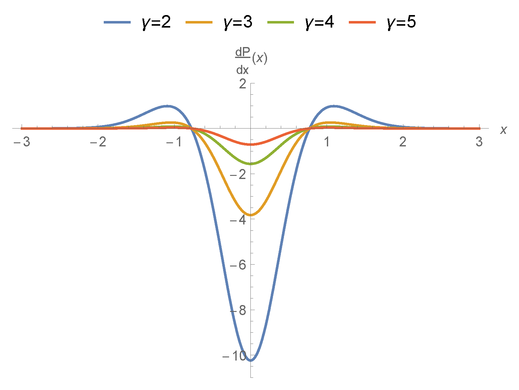
• The gradients of pressures in the mid region are going up because of sturdy applied stress.
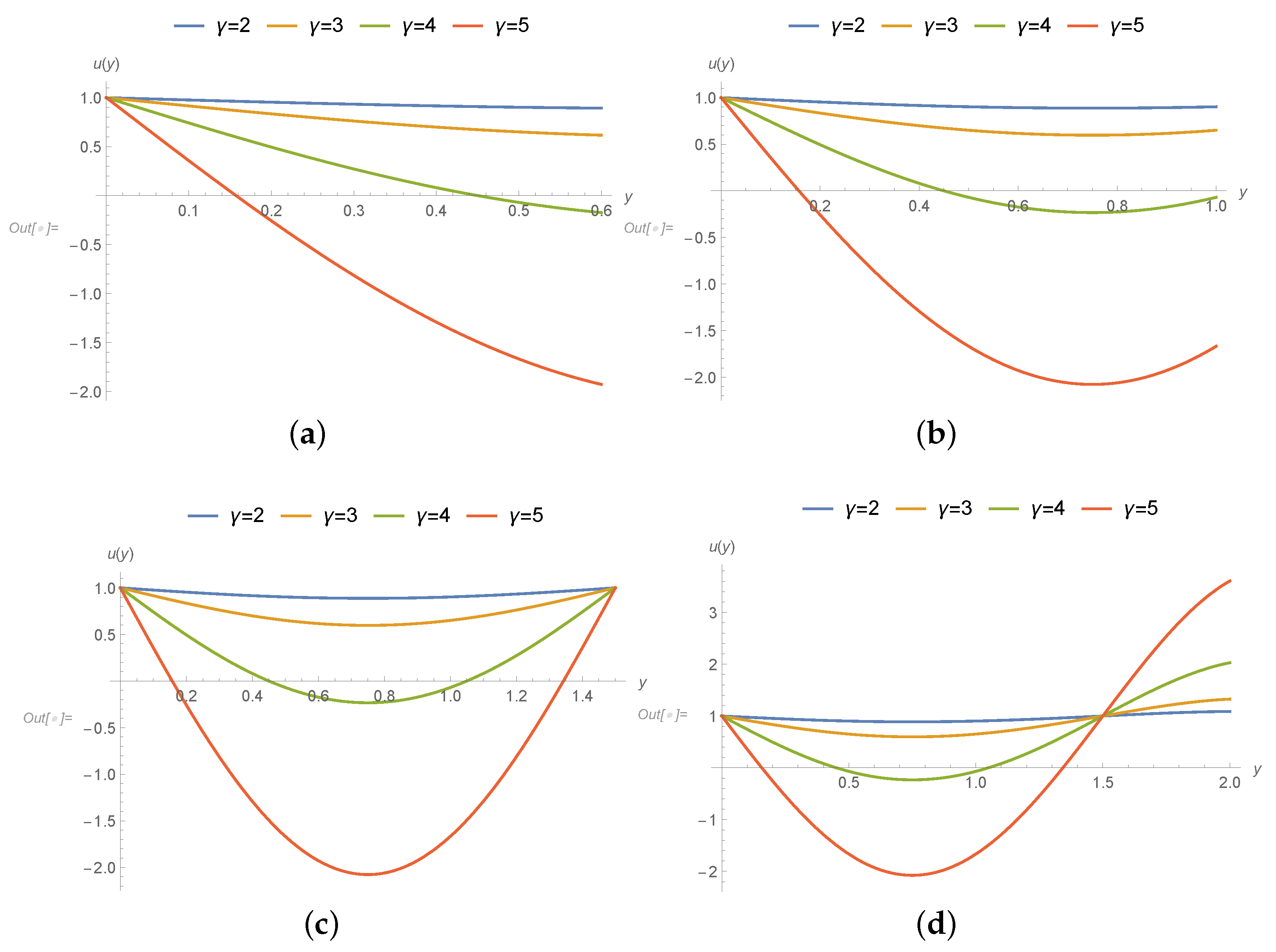
• In the upper stream and downwards sections of graphs, velocity and transport properties have been influenced and affected largely in the middle nip section the drag flow is supported due to the poignant roller and sheet.
• The support or disagreement enhances as coupled stress rises. So the speed of coating at this position exceeds one over the whole cross-section.
• Pressure slope is upbeat and as a consequence the speed at this position is utmost at the joining section of roller and leaf. It is interesting to say that axial position is less affected due to applied stresses and speed of roller.

References

1. Middleman, S. Fundamentals of Polymer Processing; McGraw-Hill: New York, NY, USA, 1977. [Google Scholar]
2. Bird, R.B.; Dai, G.C.; Yarusso, B.J. The rheology and flow of viscoplastic materials. Rev. Chem. Eng. 1983, 1, 1–70. [Google Scholar] [CrossRef]
3. Greener, Y.; Middleman, S. A theory of roll coating of viscous and viscoelastic fluids. Polym. Eng. Sci. 1975, 15, 1–10. [Google Scholar] [CrossRef]
4. Coyle, D.J.; Macosko, C.W.; Scriven, L.E. Film-splitting flows in forward roll coating. J. Fluid Mech. 1986, 171, 183–207. [Google Scholar] [CrossRef]
5. Hintermaier, J.C.; White, R.E. The splitting of a water film between rotating rolls. TAPPI J. 1965, 48, 617–625. [Google Scholar]
6. Benkreira, H.; Patel, R.; Edwards, M.F.; Wilkinson, W.L. Classification and analyses of coating flows. J. Non-Newton. Fluid Mech. 1994, 54, 437–447. [Google Scholar] [CrossRef] [Green Version]
7. Benkreira, H.; Edwards, M.F.; Wilkinson, W.L. Roll coating of purely viscous liquids. Chem. Eng. Sci. 1981, 36, 429–434. [Google Scholar] [CrossRef]
8. Benkreira, H.; Edwards, M.F.; Wilkinson, W.L. Roll coating operations. J. Non-Newton. Fluid Mech. 1984, 14, 377–389. [Google Scholar] [CrossRef]
9. Benkreira, H.; Edwards, M.F.; Wilkinson, W.L. A semi-empirical model of the forward roll coating flow of Newtonian fluids. Chem. Eng. Sci. 1981, 36, 423–427. [Google Scholar] [CrossRef]
10. Sofou, S.; Mitsoulis, E. Roll-over-web coating of pseudoplastic and viscoplastic sheets using the lubrication approximation. J. Plast. Film Sheet. 2005, 21, 307–333. [Google Scholar] [CrossRef]
11. Zahid, M.; Haroon, T.; Rana, M.A.; Siddiqui, A.M. Roll coating analysis of a third grade fluid. J. Plast. Film Sheet. 2017, 33, 72–91. [Google Scholar] [CrossRef]
12. Zahid, M.; Rana, M.A.; Siddiqui, A.M. Roll coating analysis of a second-grade material. J. Plast. Film Sheet. 2018, 34, 232–255. [Google Scholar] [CrossRef]
13. Ali, N.; Atif, H.M.; Javed, M.A.; Sajid, M. A theoretical analysis of roll-over-web coating of couple stress fluid. J. Plast. Film Sheet. 2018, 34, 43–59. [Google Scholar] [CrossRef] [Green Version]
14. Gaskell, P.H.; Savage, M.D.; Summers, J.L.; Thompson, H.M. Modelling and analysis of meniscus roll coating. J. Fluid Mech. 1995, 298, 113–137. [Google Scholar] [CrossRef]
15. Marinca, V.; Herisanu, N. Determination of periodic solutions for the motion of a particle on a rotating parabola by means of the optimal homotopy asymptotic method. J. Sound Vib. 2010, 329, 1450–1459. [Google Scholar] [CrossRef]
16. Iqbal, S.; Idrees, M.; Siddiqui, A.M.; Ansari, A.R. Some solutions of the linear and nonlinear Klein–Gordon equations using the optimal homotopy asymptotic method. Appl. Math. Comput. 2010, 216, 2898–2909. [Google Scholar] [CrossRef]
17. Iqbal, S.; Javed, A. Application of optimal homotopy asymptotic method for the analytic solution of singular Lane–Emden type equation. Appl. Math. Comput. 2011, 217, 7753–7761. [Google Scholar] [CrossRef]
18. Iqbal, S.; Ansari, A.R.; Siddiqui, A.M.; Javed, A. Use of optimal homotopy asymptotic method and Galerkin’s finite element formulation in the study of heat transfer flow of a third grade fluid between parallel plates. J. Heat Transf. 2011, 133, 091702. [Google Scholar] [CrossRef]
19. Hashmi, M.S.; Khan, N.; Iqbal, S. Numerical solutions of weakly singular Volterra integral equations using the optimal homotopy asymptotic method. Comput. Math. Appl. 2012, 64, 1567–1574. [Google Scholar] [CrossRef] [Green Version]
20. Hashmi, M.S.; Khan, N.; Iqbal, S. Optimal homotopy asymptotic method for solving nonlinear Fredholm integral equations of second kind. Appl. Math. Comput. 2012, 218, 10982–10989. [Google Scholar] [CrossRef]
21. Khaliq, S.; Abbas, Z. A theoretical analysis of roll-over-web coating assessment of viscous nanofluid containing Cu-water nanoparticles. J. Plast. Film Sheet. 2020, 36, 55–75. [Google Scholar] [CrossRef]
22. Atif, H.M.; Ali, N.; Javed, M.A.; Abbas, F. Theoretical analysis of roll-over-web coating of a micropolar fluid under lubrication approximation theory. J. Plast. Film Sheet. 2018, 34, 418–438. [Google Scholar] [CrossRef]
23. Bhatti, S.; Zahid, M.; Rana, M.A.; Siddiqui, A.M.; Abdul Wahab, H. Numerical analysis of blade coating of a third-order fluid. J. Plast. Film Sheet. 2019, 35, 157–180. [Google Scholar] [CrossRef]
24. Siddiqui, A.M.; Zahid, M.; Rana, M.A.; Haroon, T. Calendering analysis of a third-order fluid. J. Plast. Film Sheet. 2014, 30, 345–368. [Google Scholar] [CrossRef]
25. Singh, B. Wave propagation in a generalized thermoelastic material with voids. Appl. Math. Comput. 2007, 189, 698–709. [Google Scholar] [CrossRef]
26. Mallik, S.H.; Kanoria, M. Generalized thermoelastic functionally graded solid with a periodically varying heat source. Int. J. Solids Struct. 2007, 44, 7633–7645. [Google Scholar] [CrossRef]
27. Blake, T.D.; Ruschak, K.J.; Kistler, S.F.; Schweizer, P.M. Liquid Film Coating; Chapman and Hall: London, UK, 1997. [Google Scholar]
28. Hayat, T.; Farooq, S.; Alsaedi, A.; Ahmad, B. Numerical study for Soret and Dufour effects on mixed convective peristalsis of Oldroyd 8-constants fluid. Int. J. Therm. Sci. 2017, 112, 68–81. [Google Scholar] [CrossRef]
29. Hwang, S.S. Non-Newtonian liquid blade coating process. J. Fluids Eng. 1982, 104, 469–474. [Google Scholar] [CrossRef]
30. Ruschak, K.J. Coating flows. Annu. Rev. Fluid Mech. 1985, 17, 65–89. [Google Scholar] [CrossRef]
Figure 1. Process of roll-coating with physical variables.
Coatings 10 00691 g001
Figure 2. Values of u at different values of γ as shown in Equations (27)–(30).
Coatings 10 00691 g002
Figure 3. Values of u in varying domain values of y at different values of γ : (a) = 0, (b) = 1, (c) = 2, (d) = 3, (e) = 4, and (f) = 5.
Coatings 10 00691 g003
Figure 4. Values of u at different values of γ as shown in Equations (31)–(34).
Coatings 10 00691 g004
Figure 5. Values of u in varying domain values of y at different values of γ : (a) = 0, (b) = 1, (c) = 2, (d) = 3, (e) = 4, and (f) = 5.
Coatings 10 00691 g005
Figure 6. Values of u at different values of γ as shown in Equations (35)–(38).
Coatings 10 00691 g006
Figure 7. Values of u in varying domain values of y at different values of γ : (a) = 0, (b) = 1, (c) = 2, (d) = 3, (e) = 4, and (f) = 5.
Coatings 10 00691 g007aCoatings 10 00691 g007b
Figure 8. Values of d P d x at different values of γ as shown in Equations (40)–(43).
Coatings 10 00691 g008
Figure 9. Values of d P d x in varying domain values of y at different values of γ : (a) = 0, (b) = 1, (c) = 2, (d) = 3, (e) = 4, and (f) = 5.
Coatings 10 00691 g009aCoatings 10 00691 g009b