
Vitreous Carbon, Geometry and Topology: A Hollistic Approach


Abstract
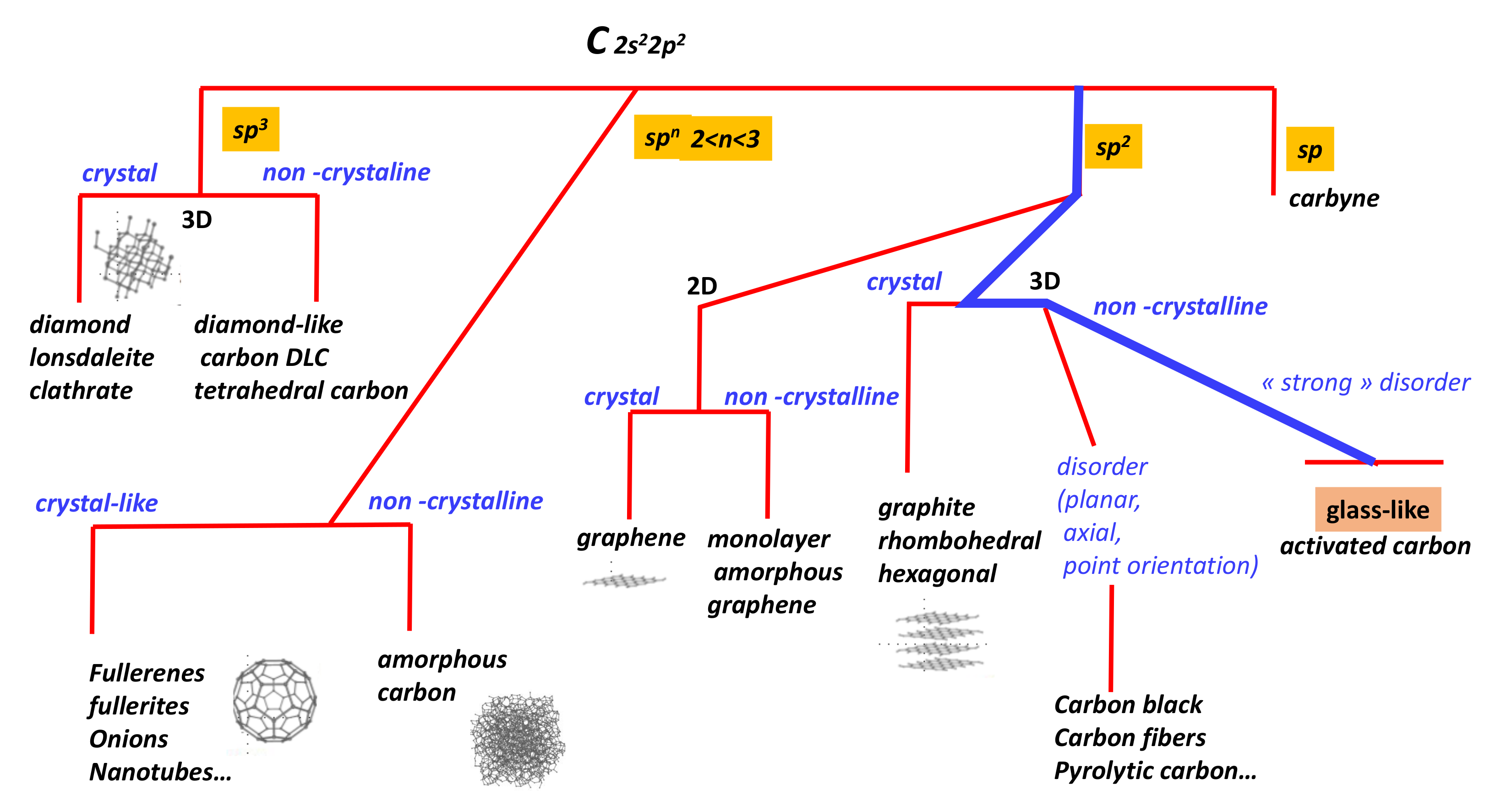
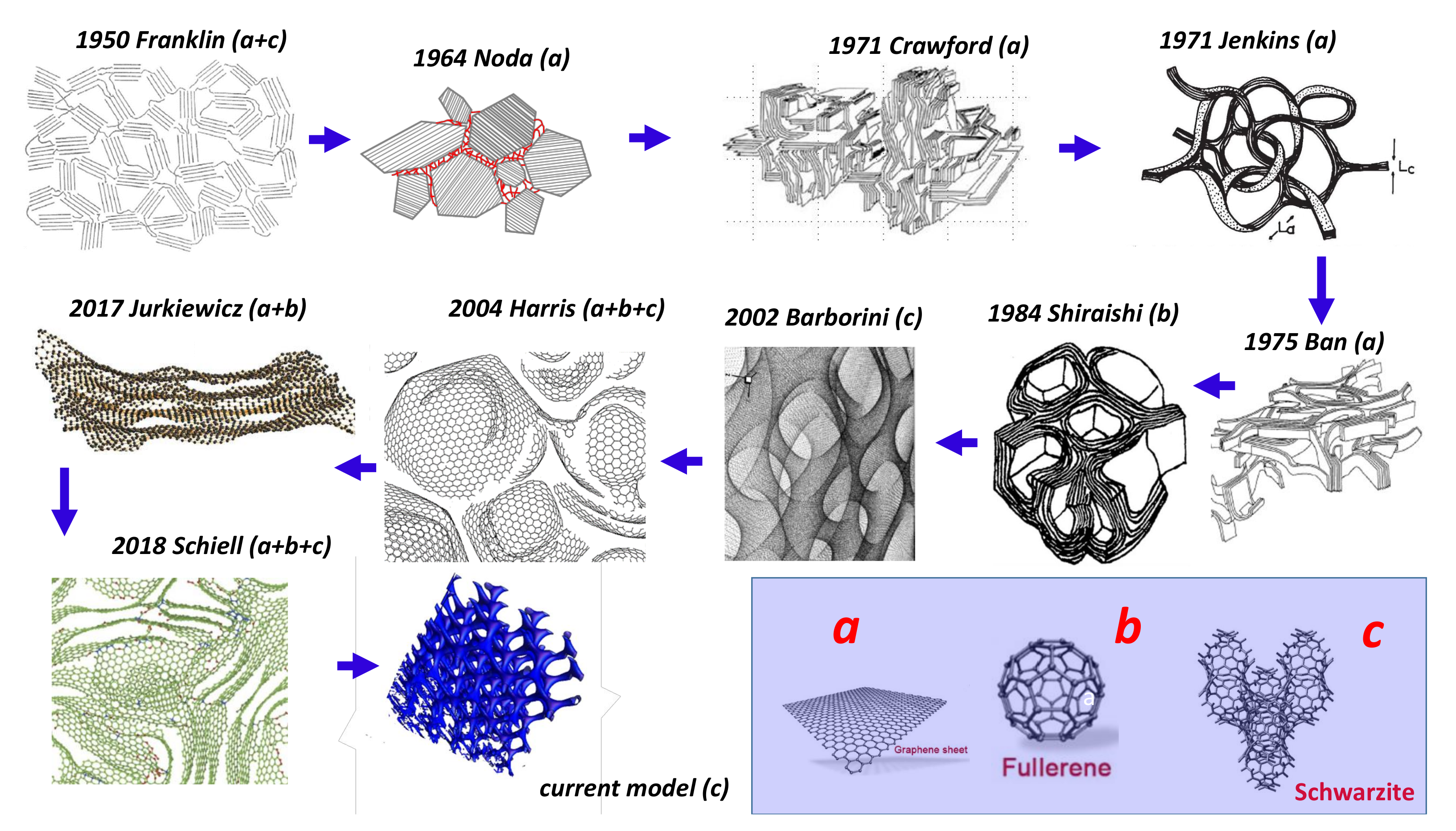
1. Introduction
2. Characterisation of GLC
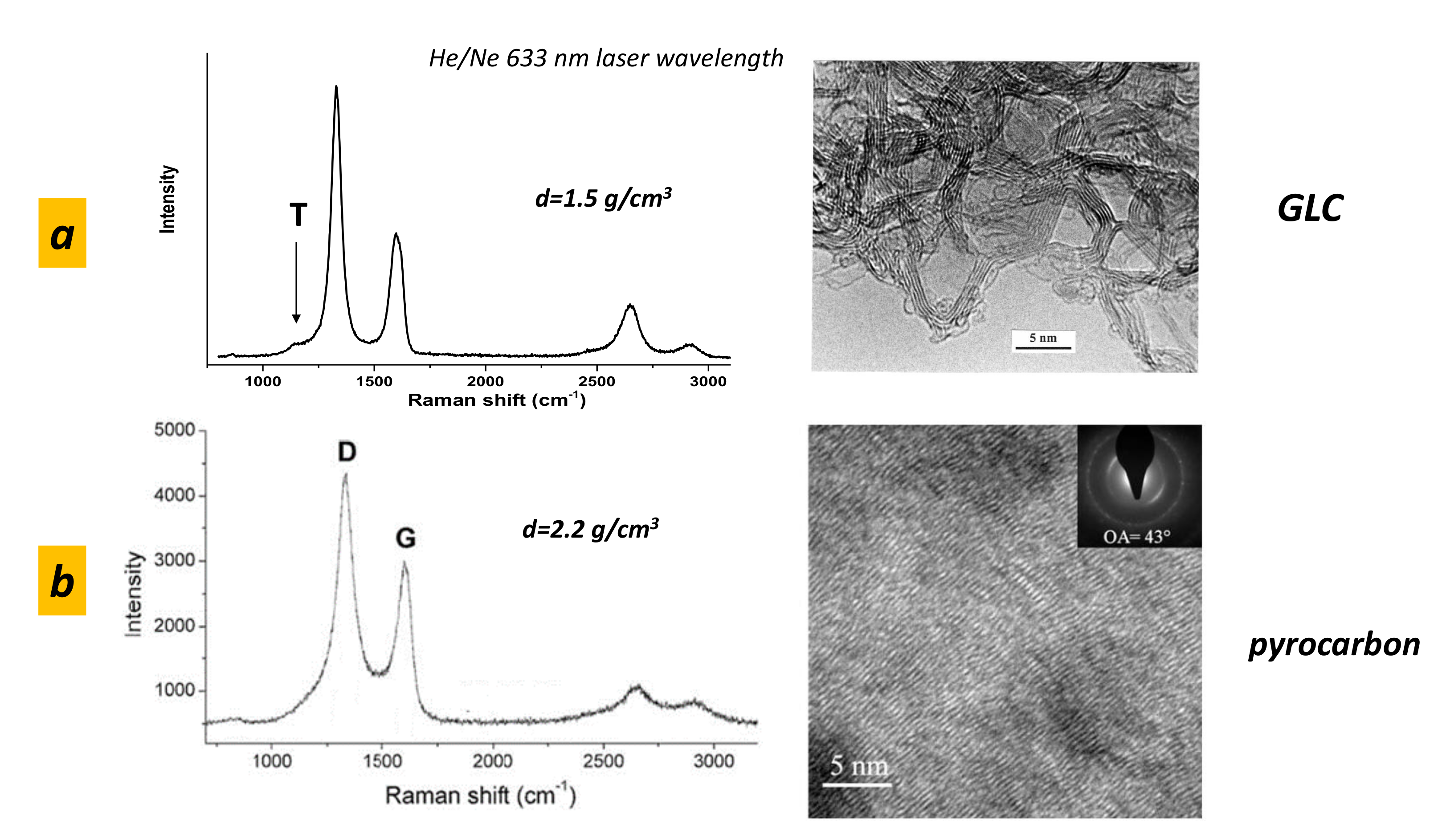
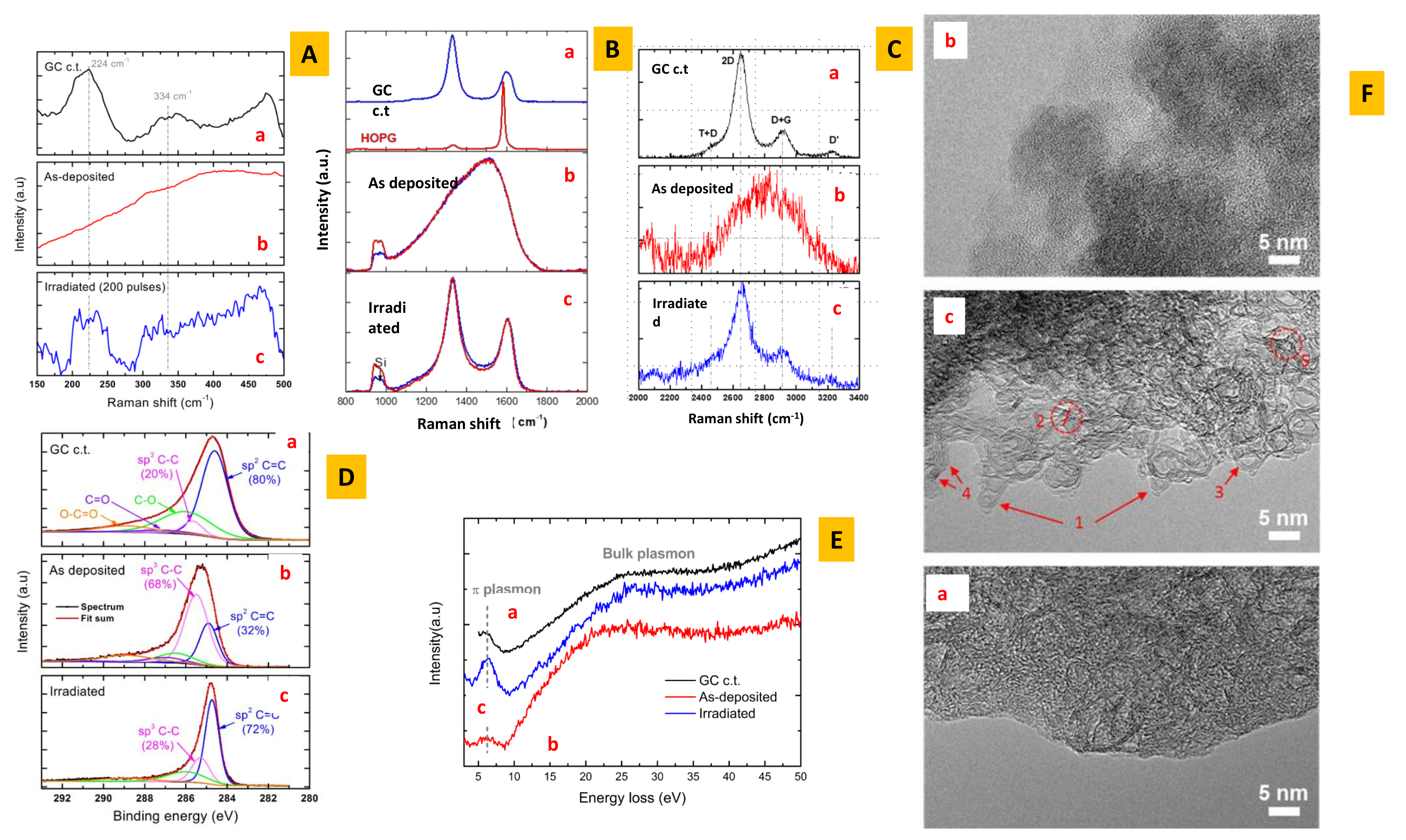
2.1. Raman Spectroscopy
2.2. Other Spectroscopies
3. Synthesis of GLC Thin Films
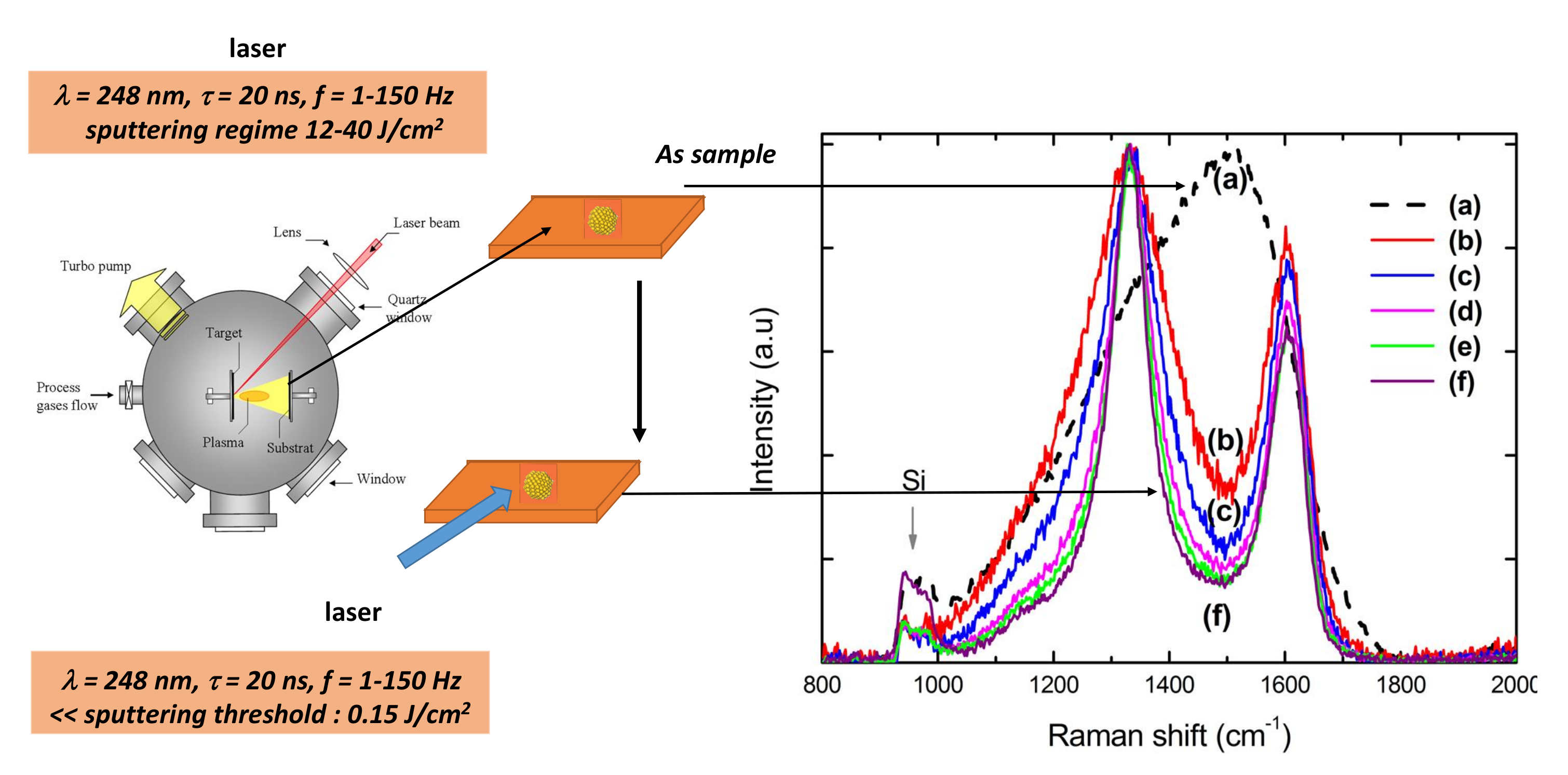
3.1. Experimental Set Up
3.2. GLC Characterisation
4. Topology/Geometry
4.1. Algebraic Topology VERSUS Geometry: From Mathematics to Physics
4.2. Dimension
4.3. Connection between Thermodynamics and Topology
4.4. Topology of Surfaces: Geometry Aspect
4.4.1. Curvature
4.4.2. Euler Characteristic
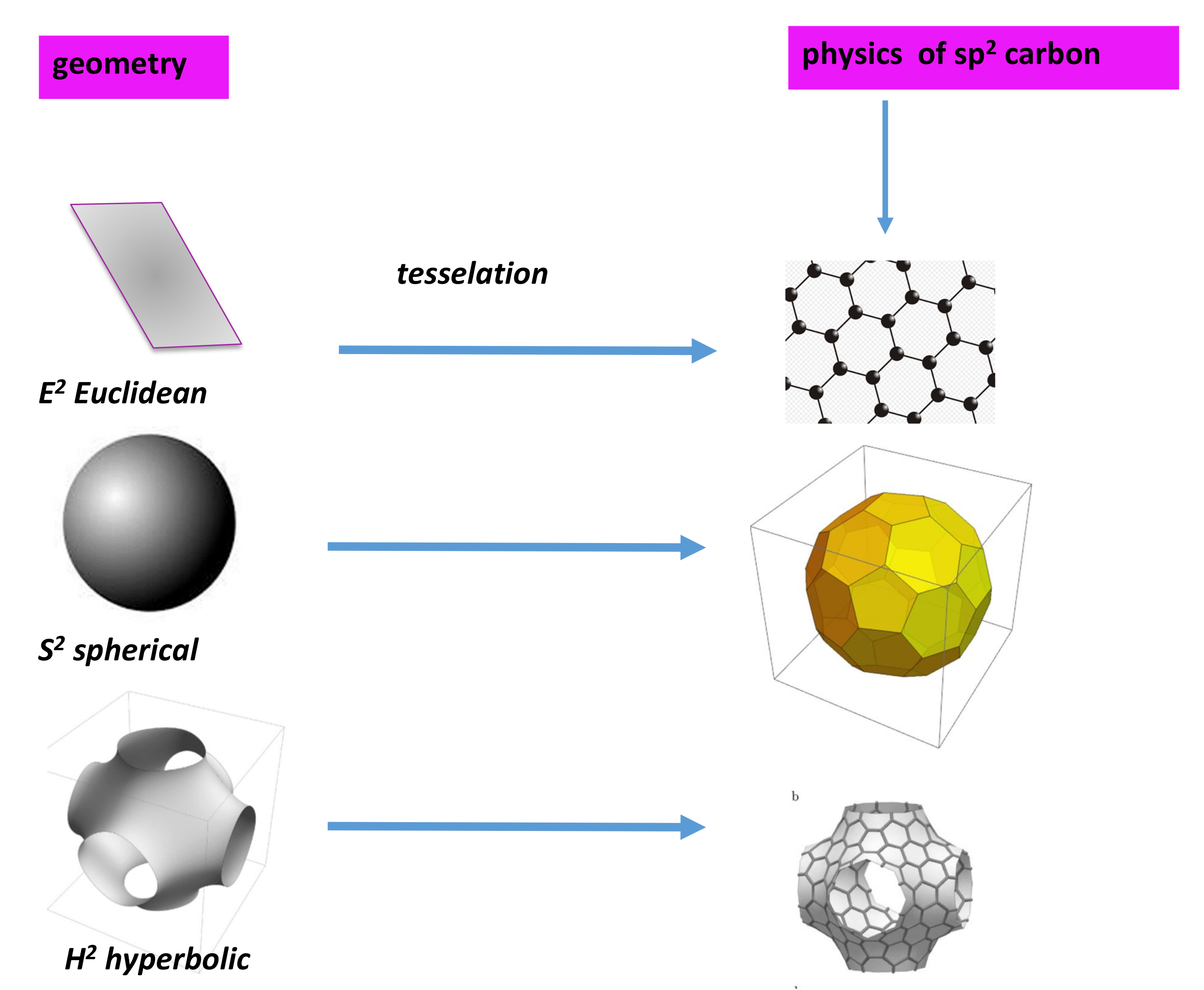
4.4.3. Geometry of 2D Surface
- (i)
- the sphere of Gaussian curvature +1;
- (ii)
- the Euclidean plane of Gaussian curvature 0; and
- (iii)
- the hyperbolic plane of Gaussian curvature −1.
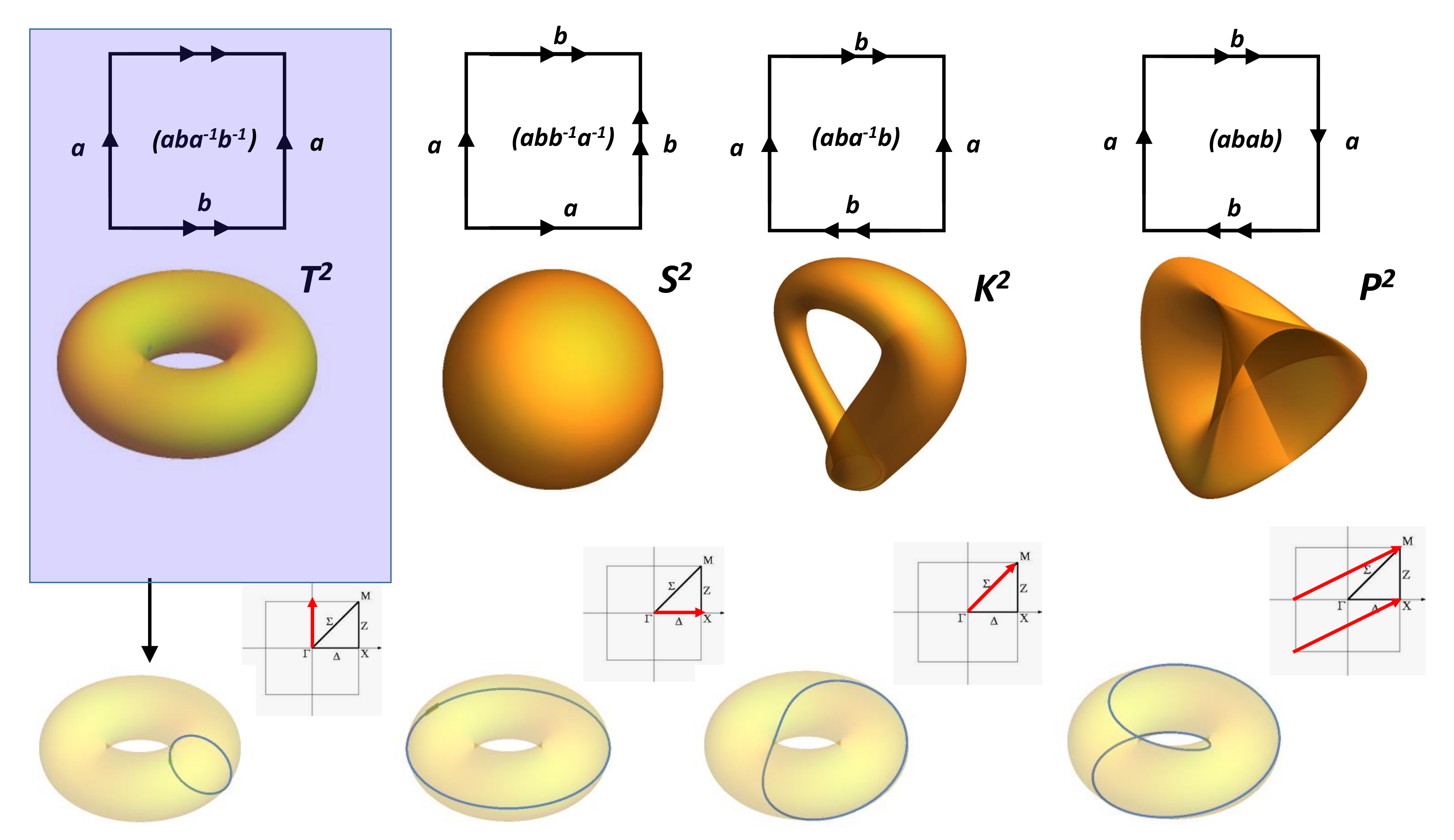
4.5. The Classification Theorem
- (i)
- a sphere;
- (ii)
- a connected sum of projective planes (if it is non-orientable); or
- (iii)
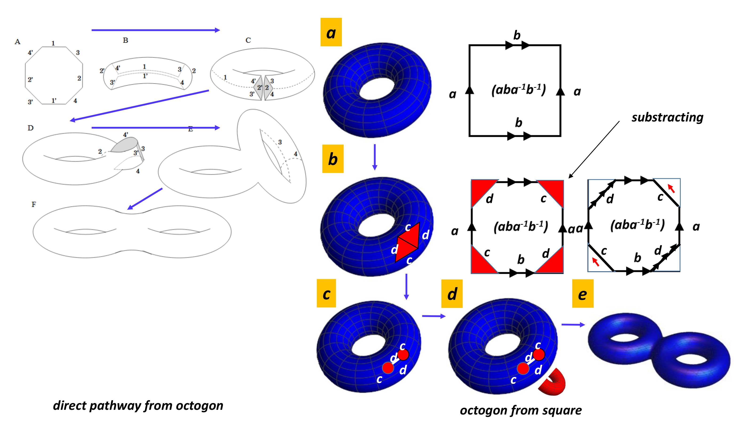
- a connected sum of torii (if it is orientable and not a sphere).
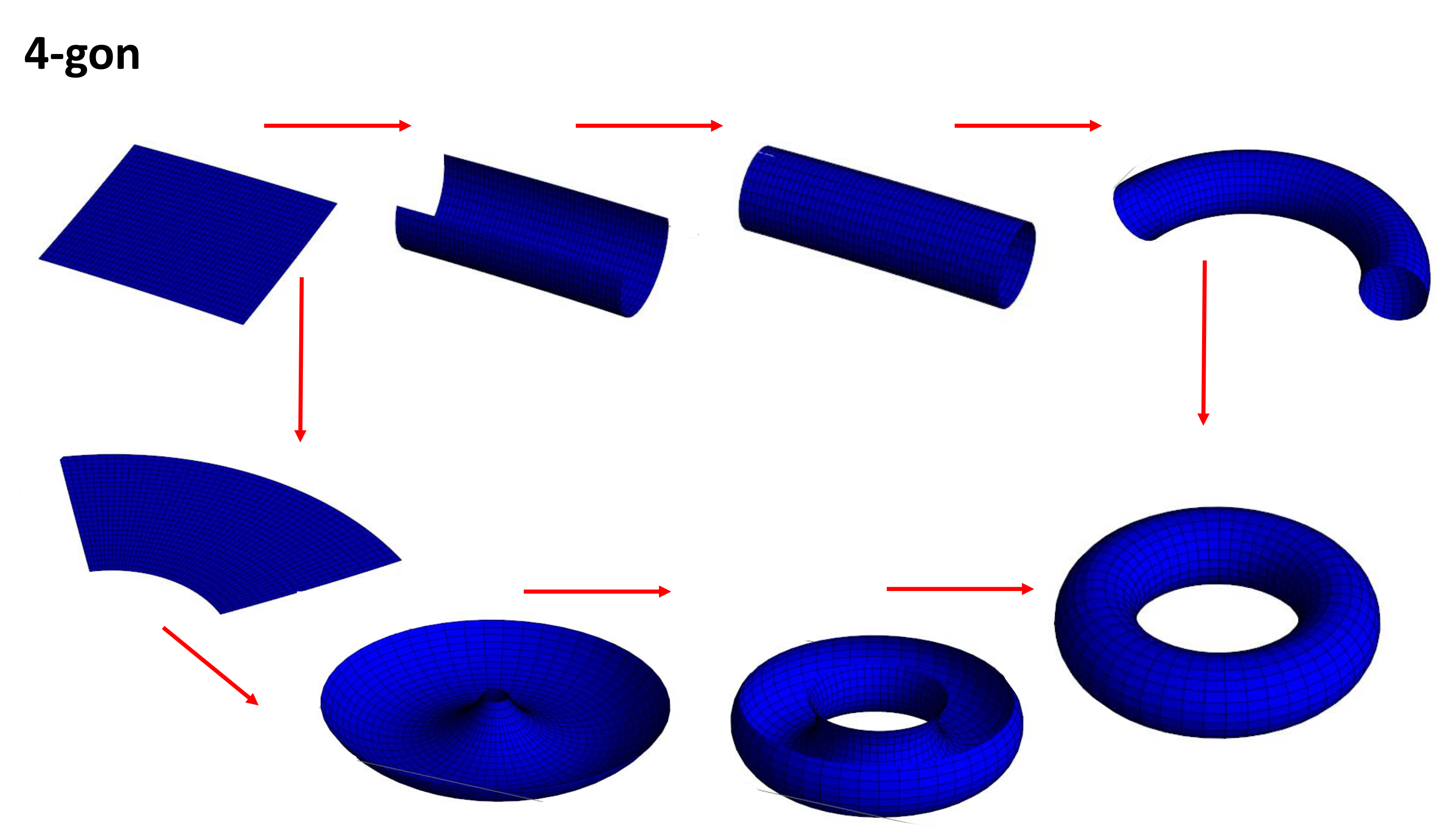
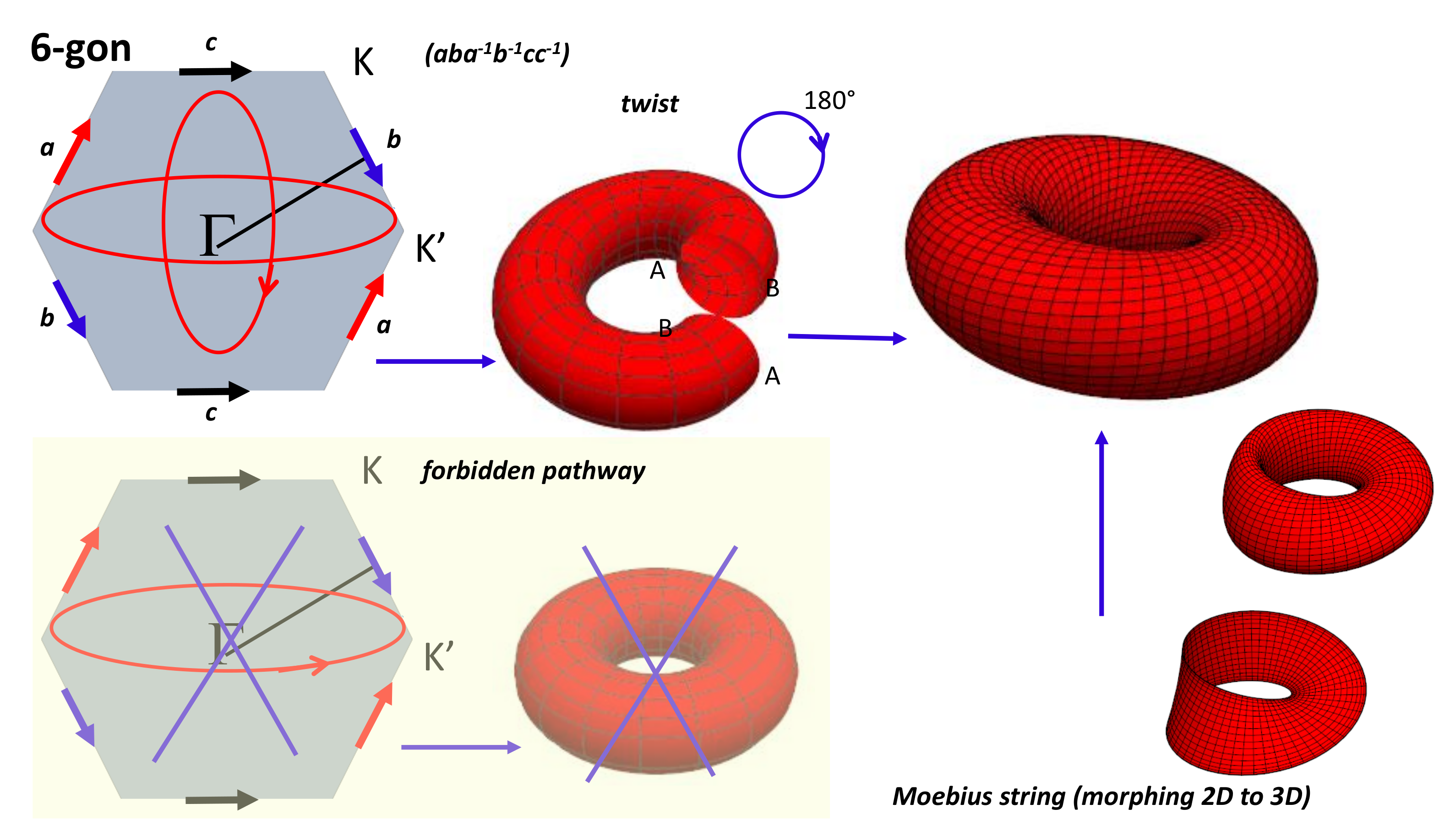
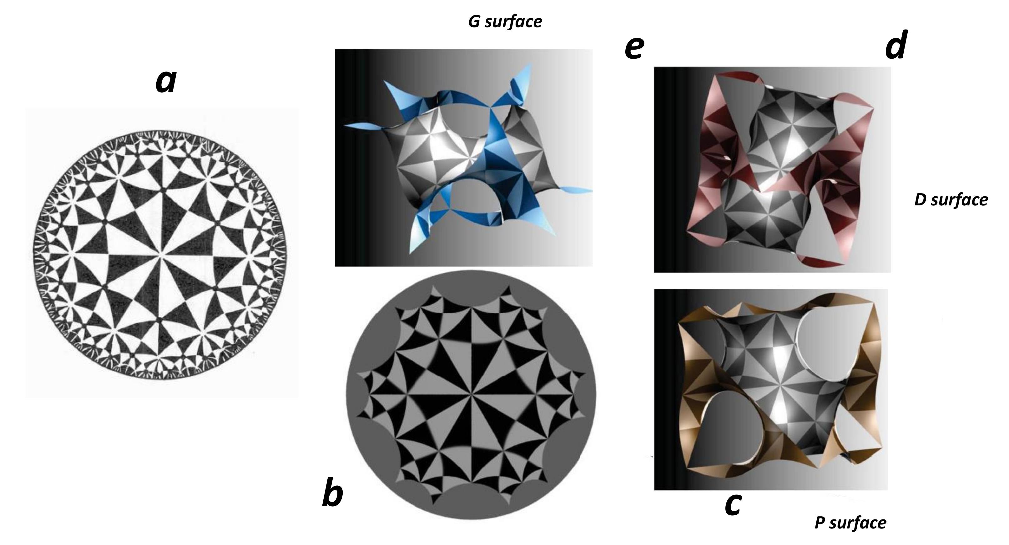
4.6. Planar Model
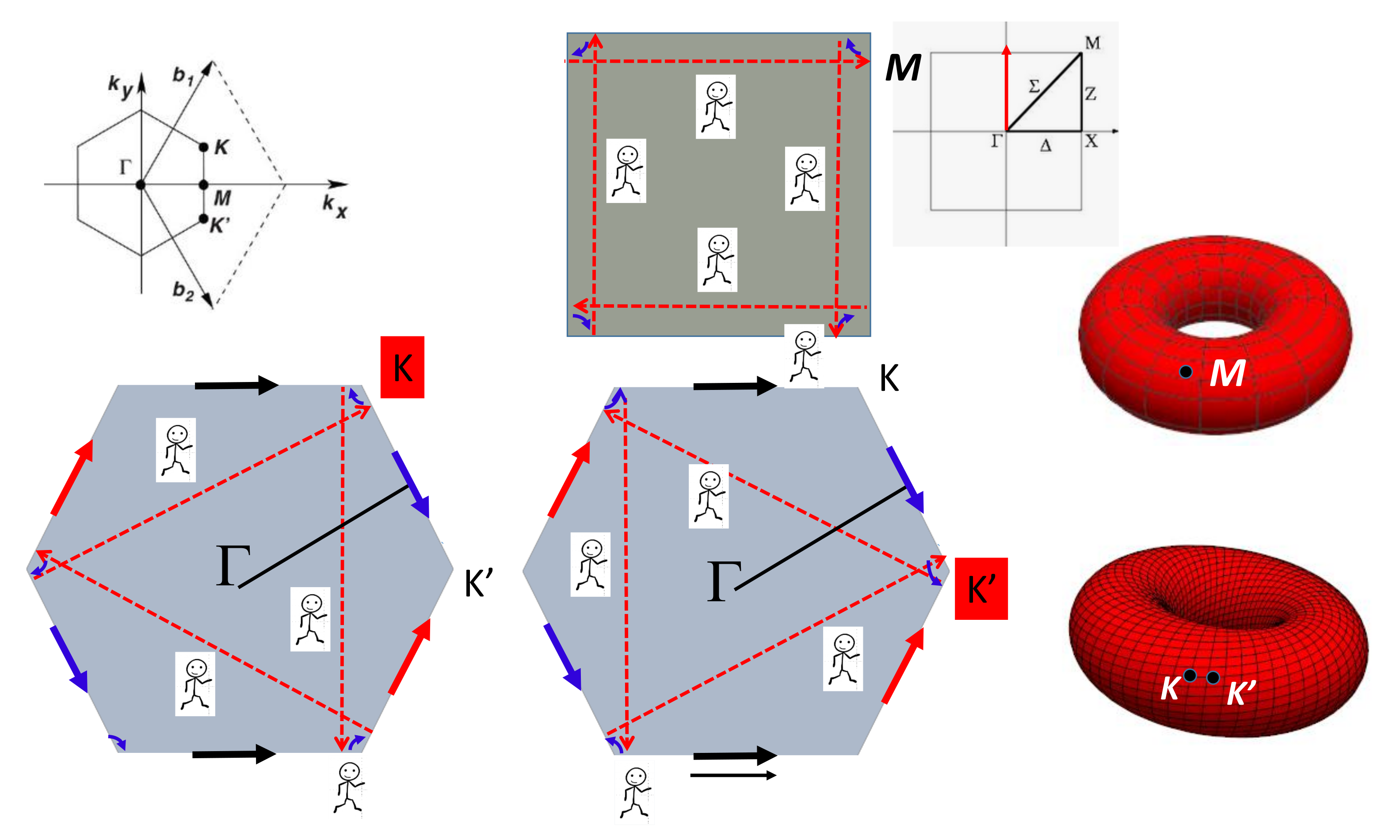
4.7. Special Points
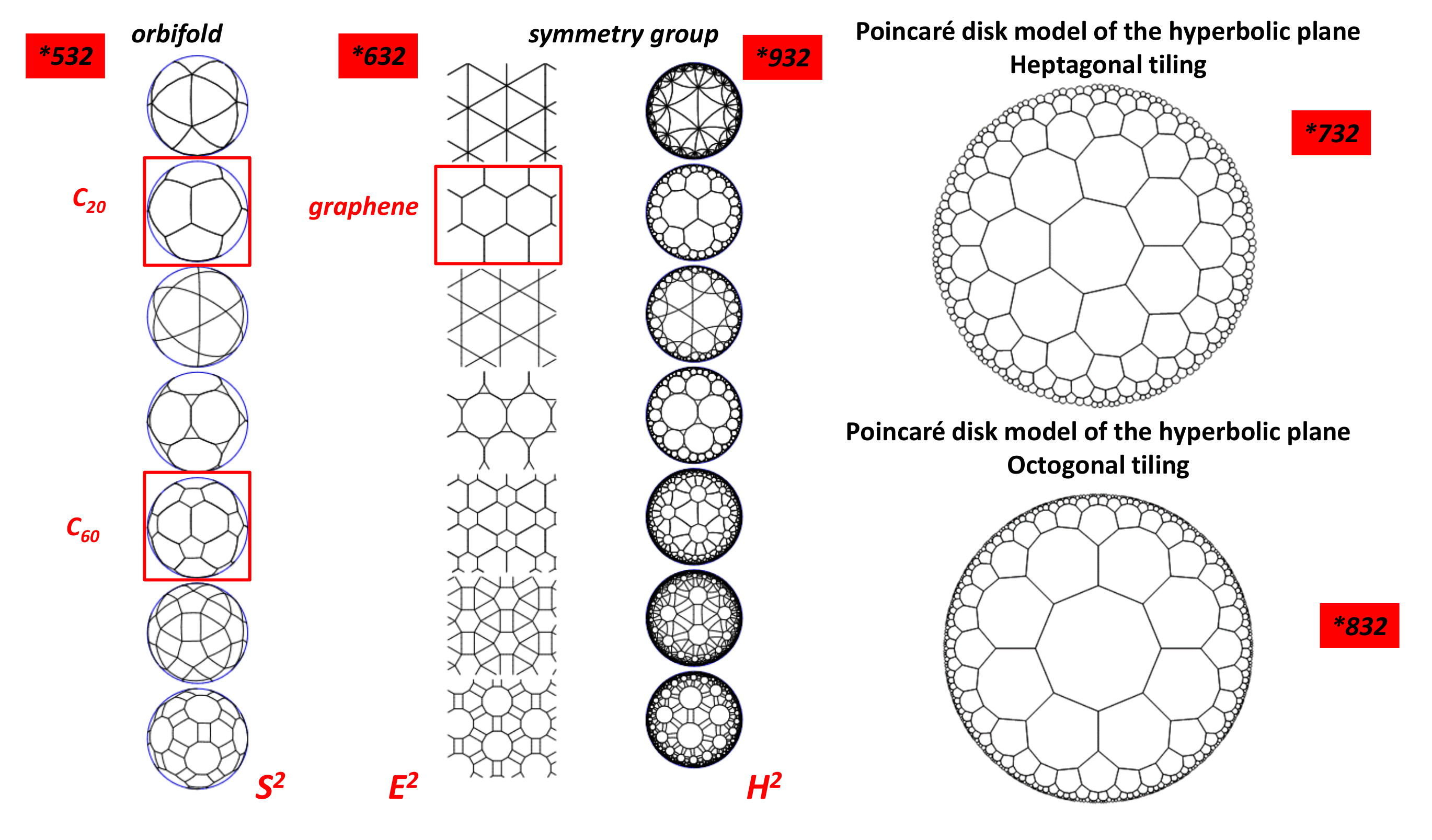
4.8. Periodicity: Space Tiling
4.8.1. The Local Gauss–Bonnet Theorem
4.8.2. 2D Crystallography
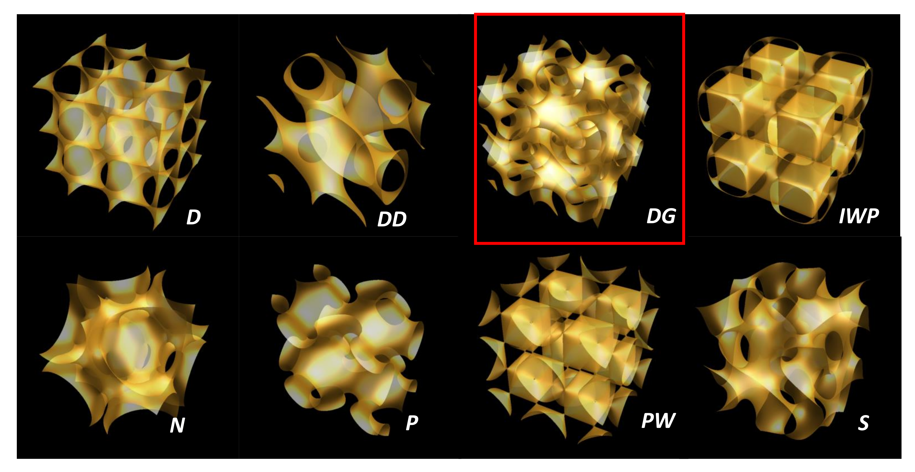
4.9. TPMS
5. GLC Properties: What Have We Learnt from Topology and Geometry
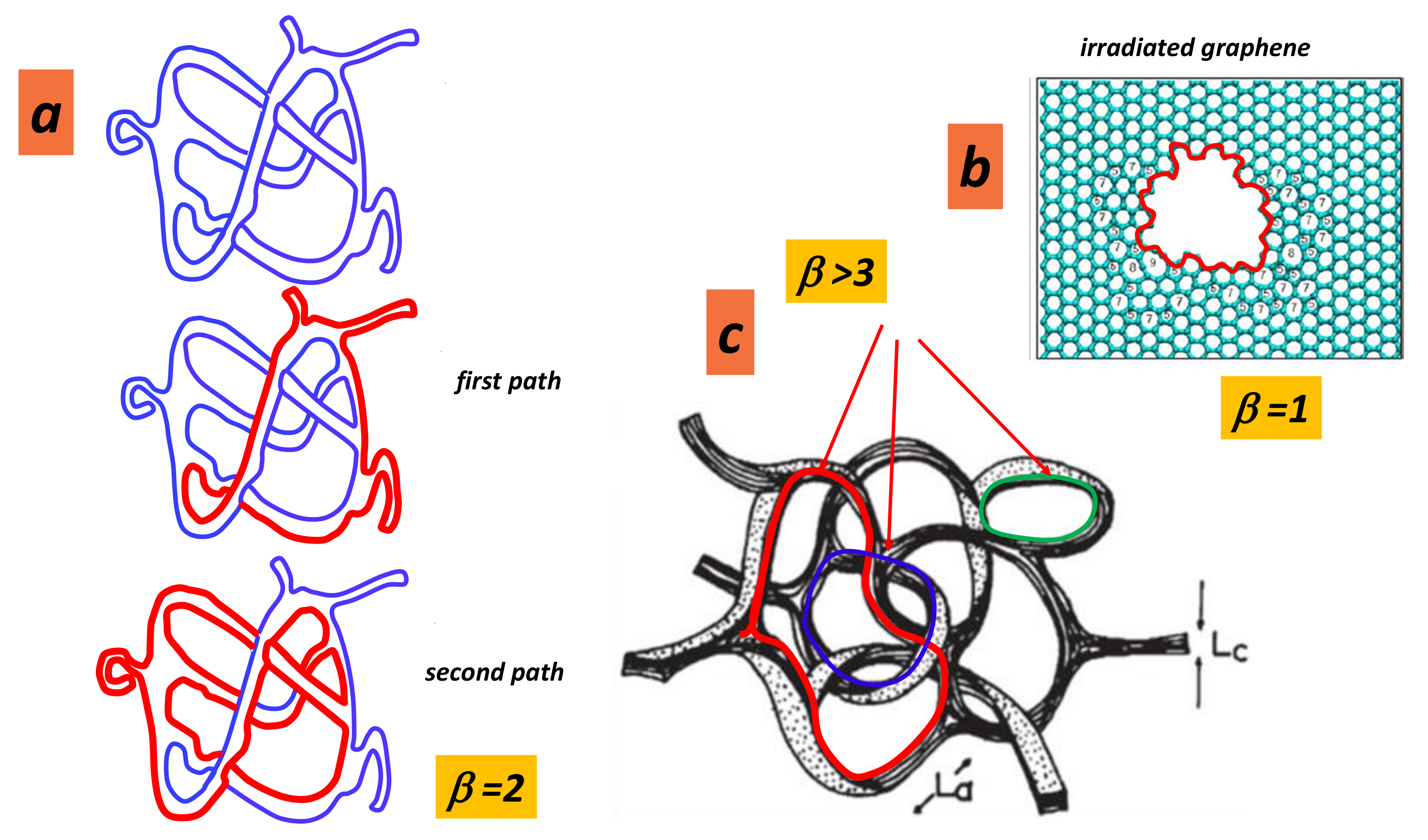
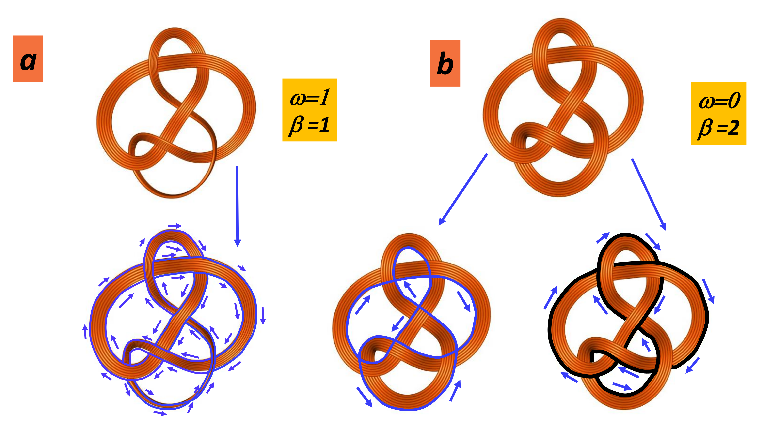
5.1. Orientability Number
5.2. Boundary Number
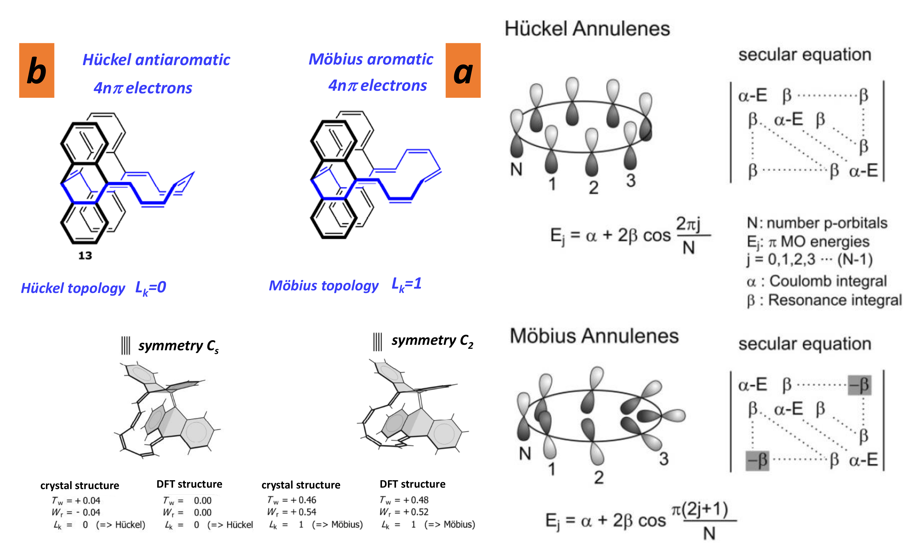
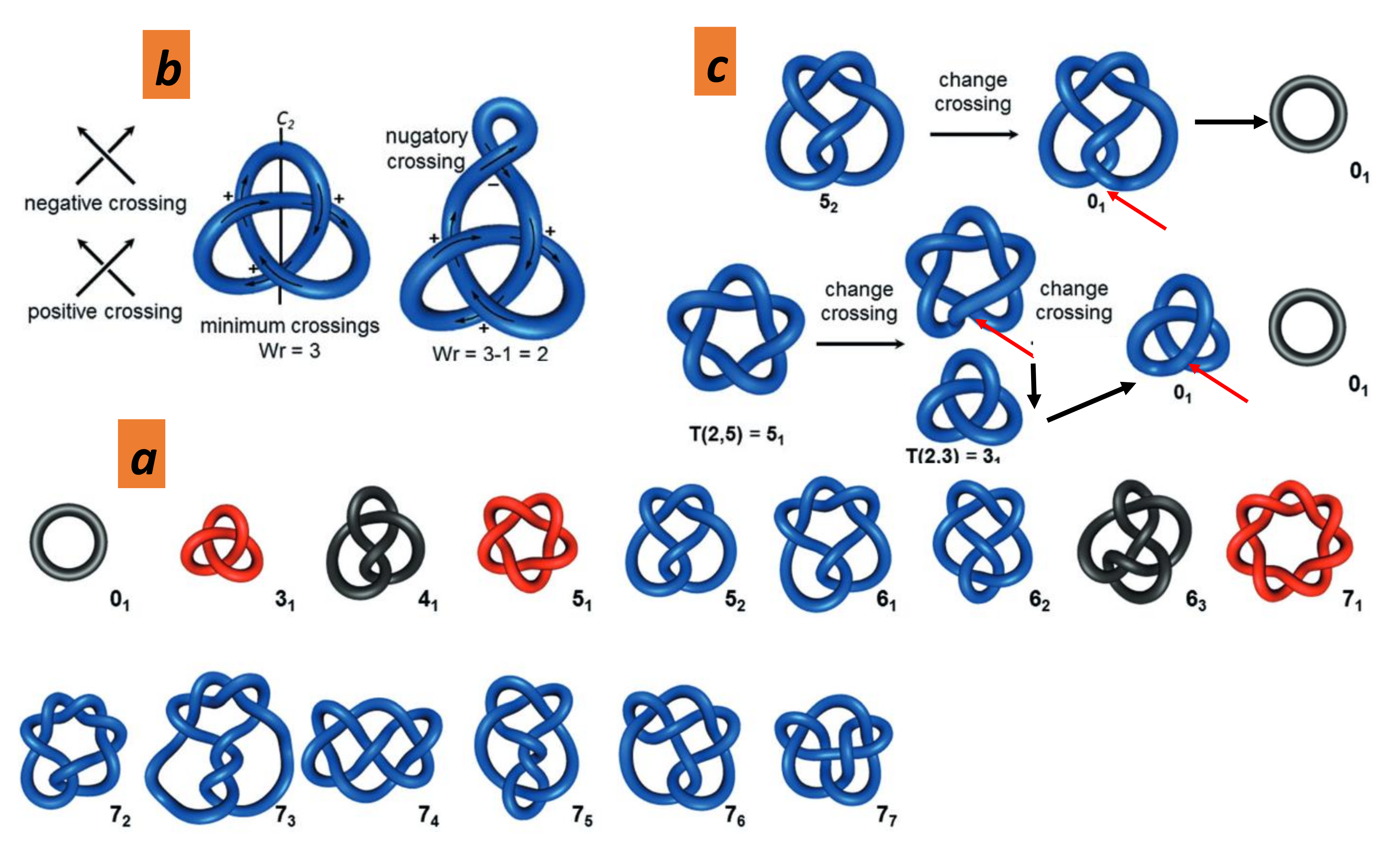
5.3. Topological Invariants from Knot Theory: Graphitisation Process
5.4. Electron Conductivity
5.5. Isotropy
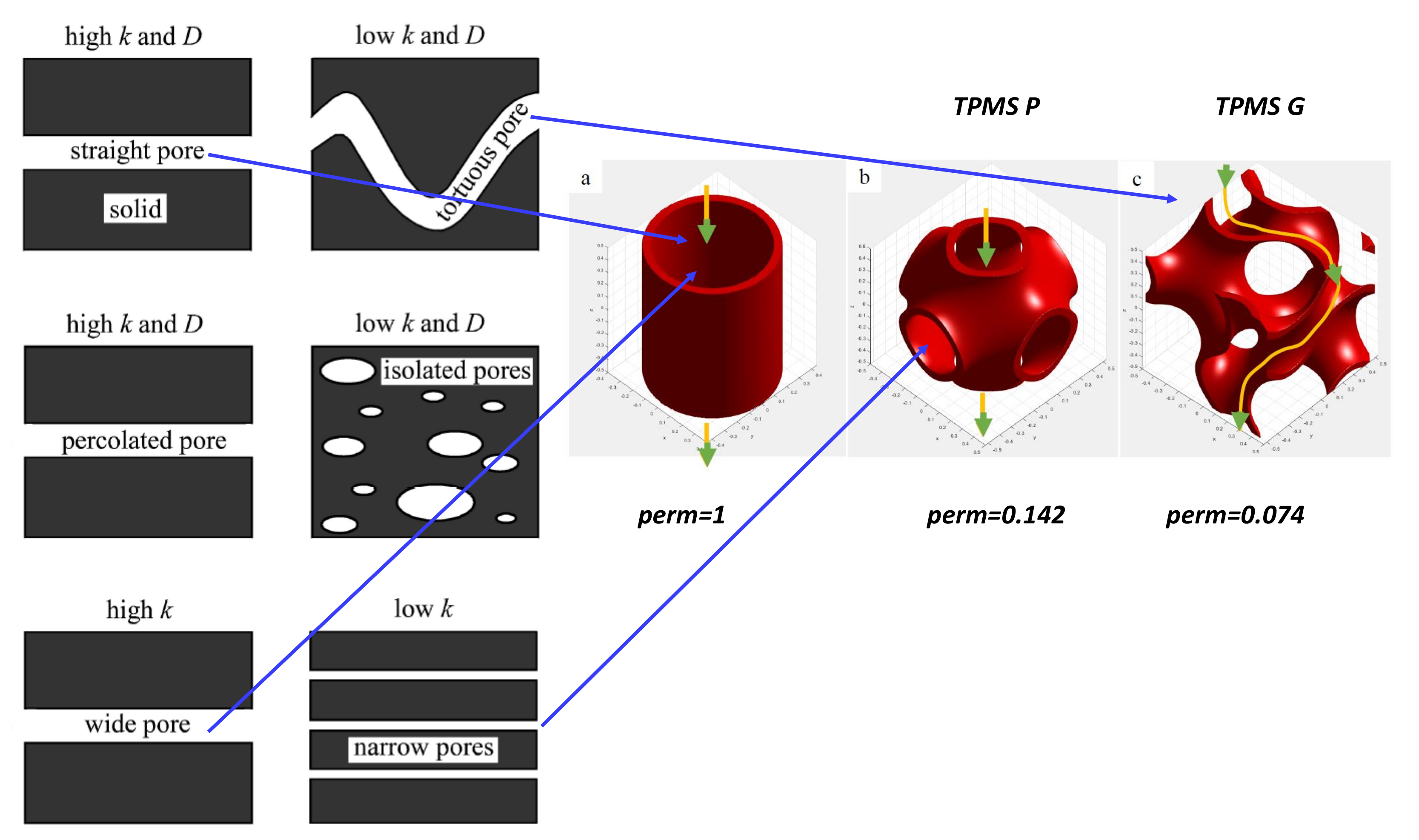
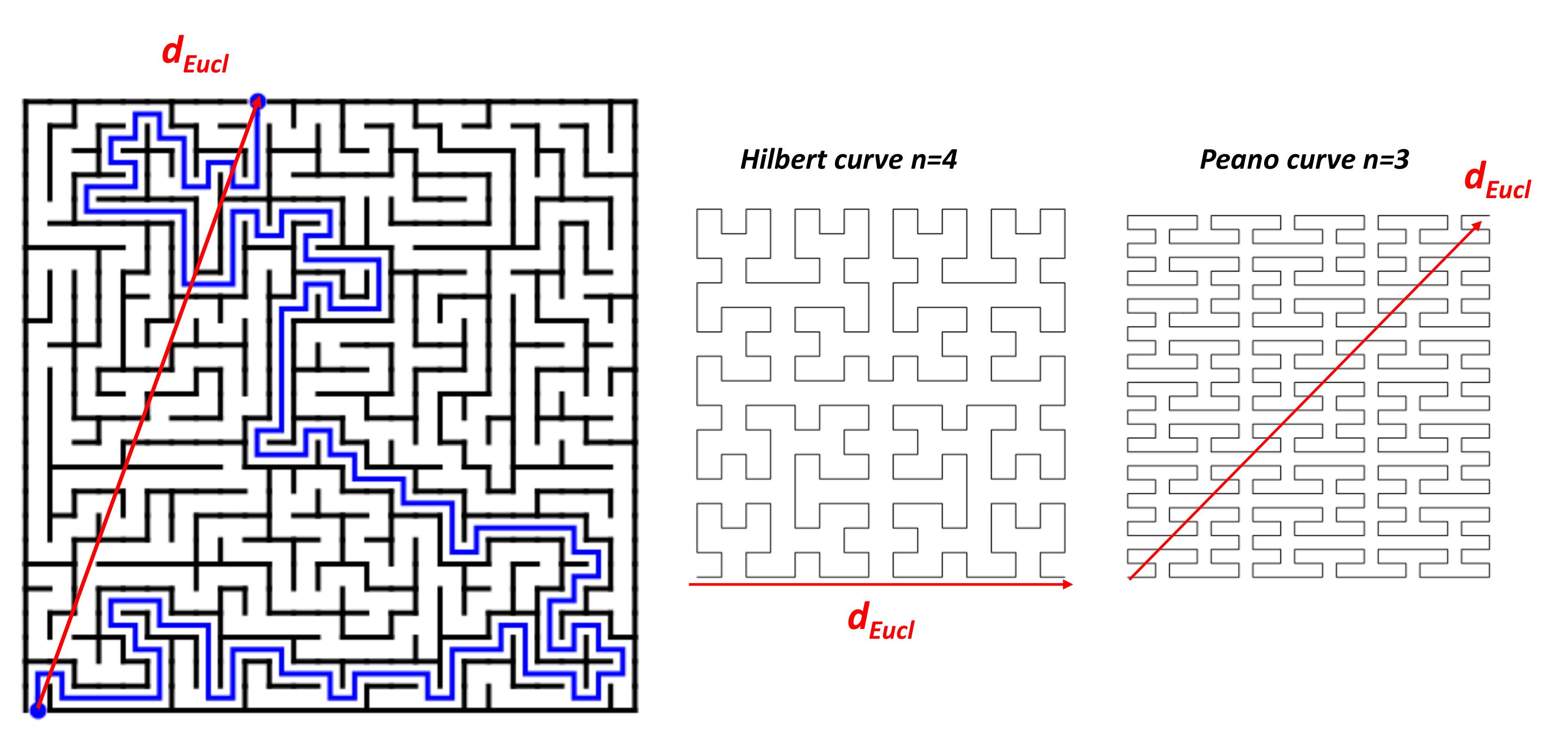
5.6. Porosity versus Gas Diffusion
5.7. GLC Stability
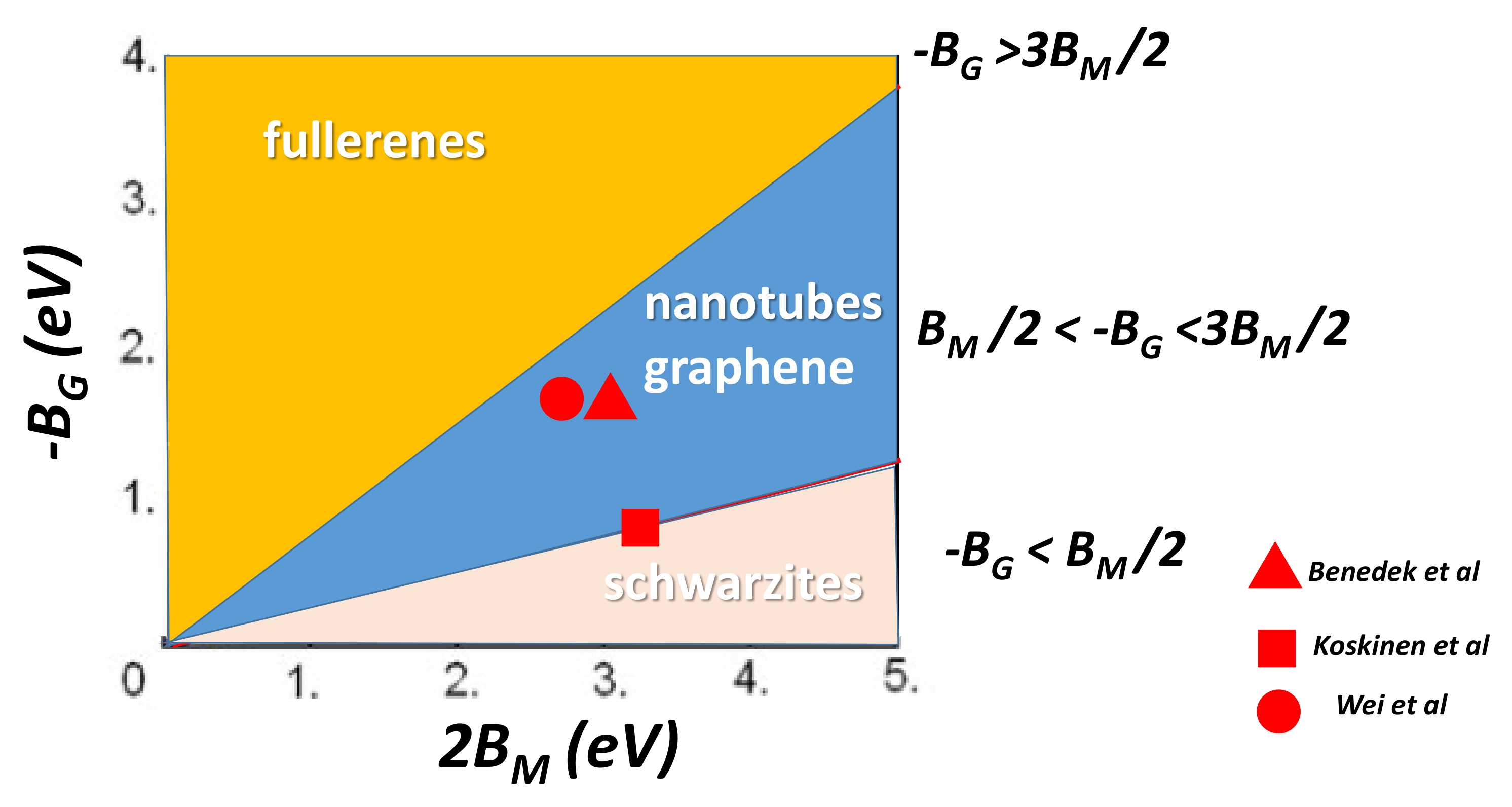
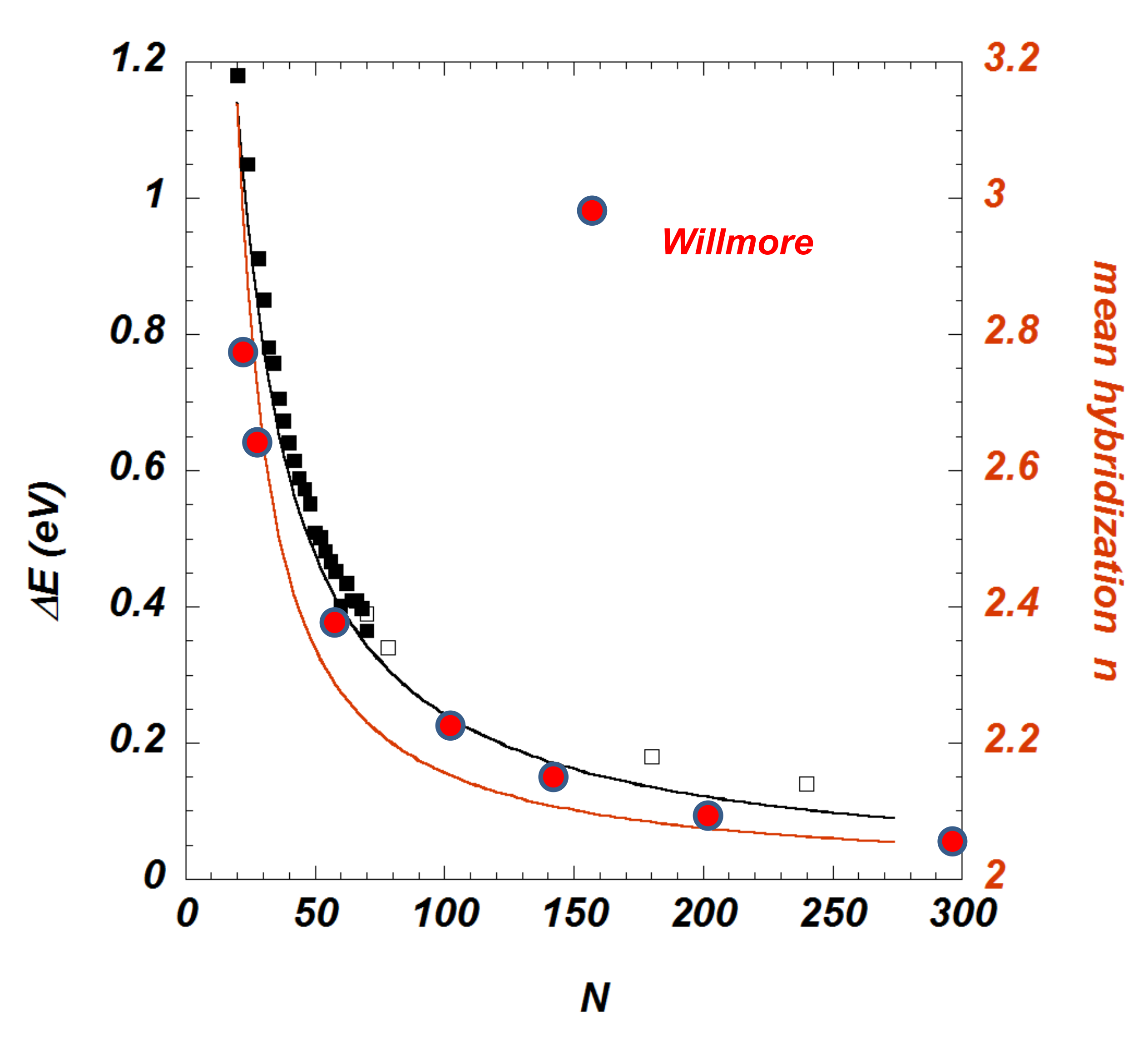
5.7.1. Willmore Energy
- -
- The graphene with then and .
- -
- The (spherical) fullerenes with everywhere, thus and , and .
- -
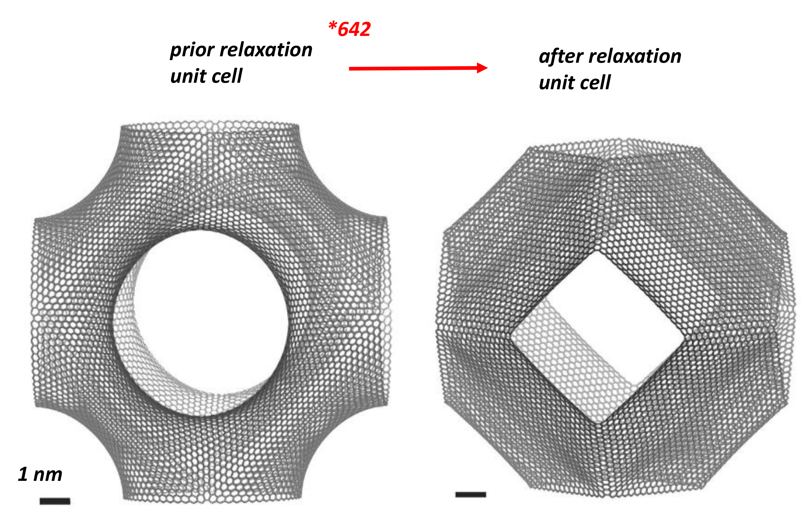
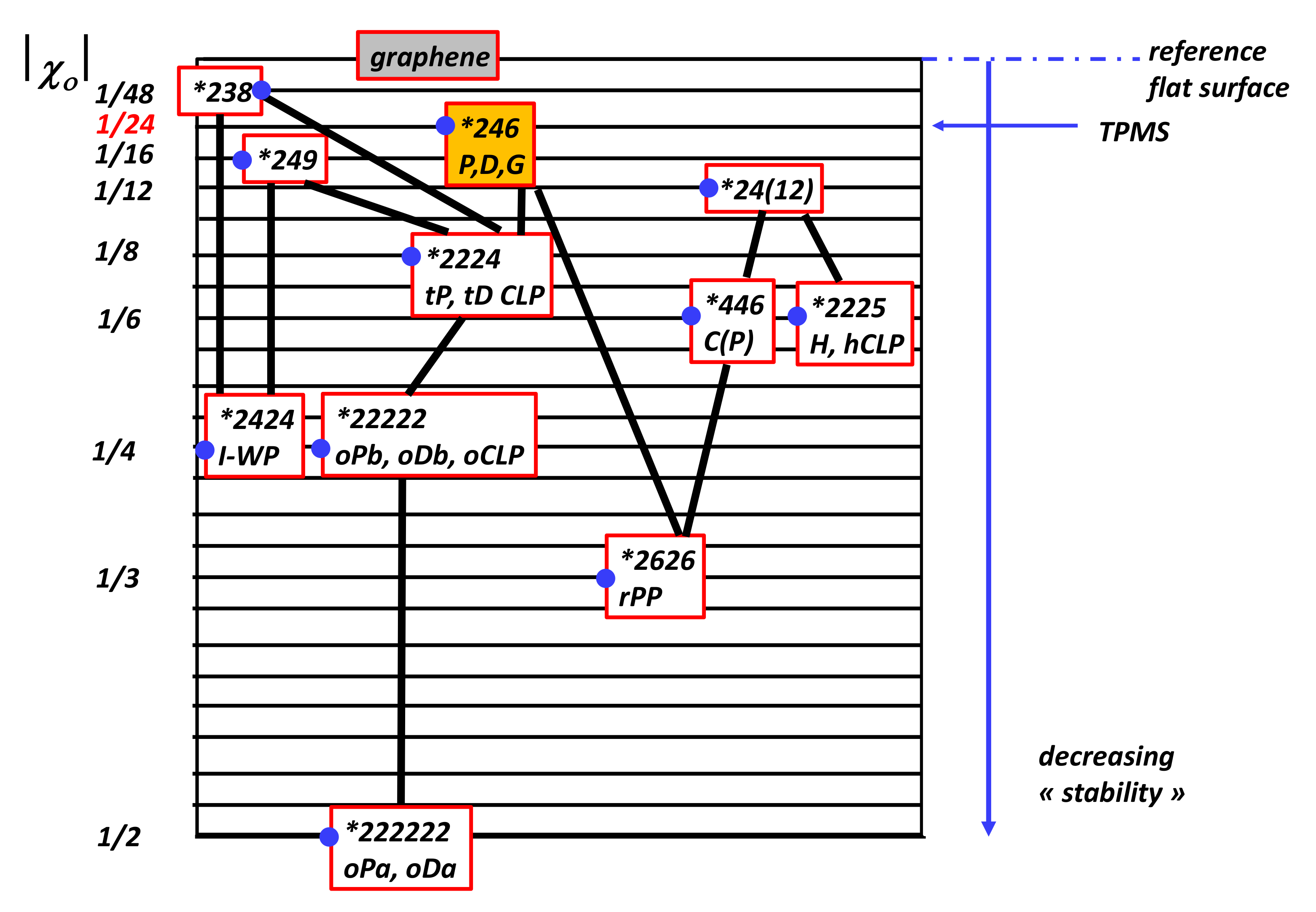
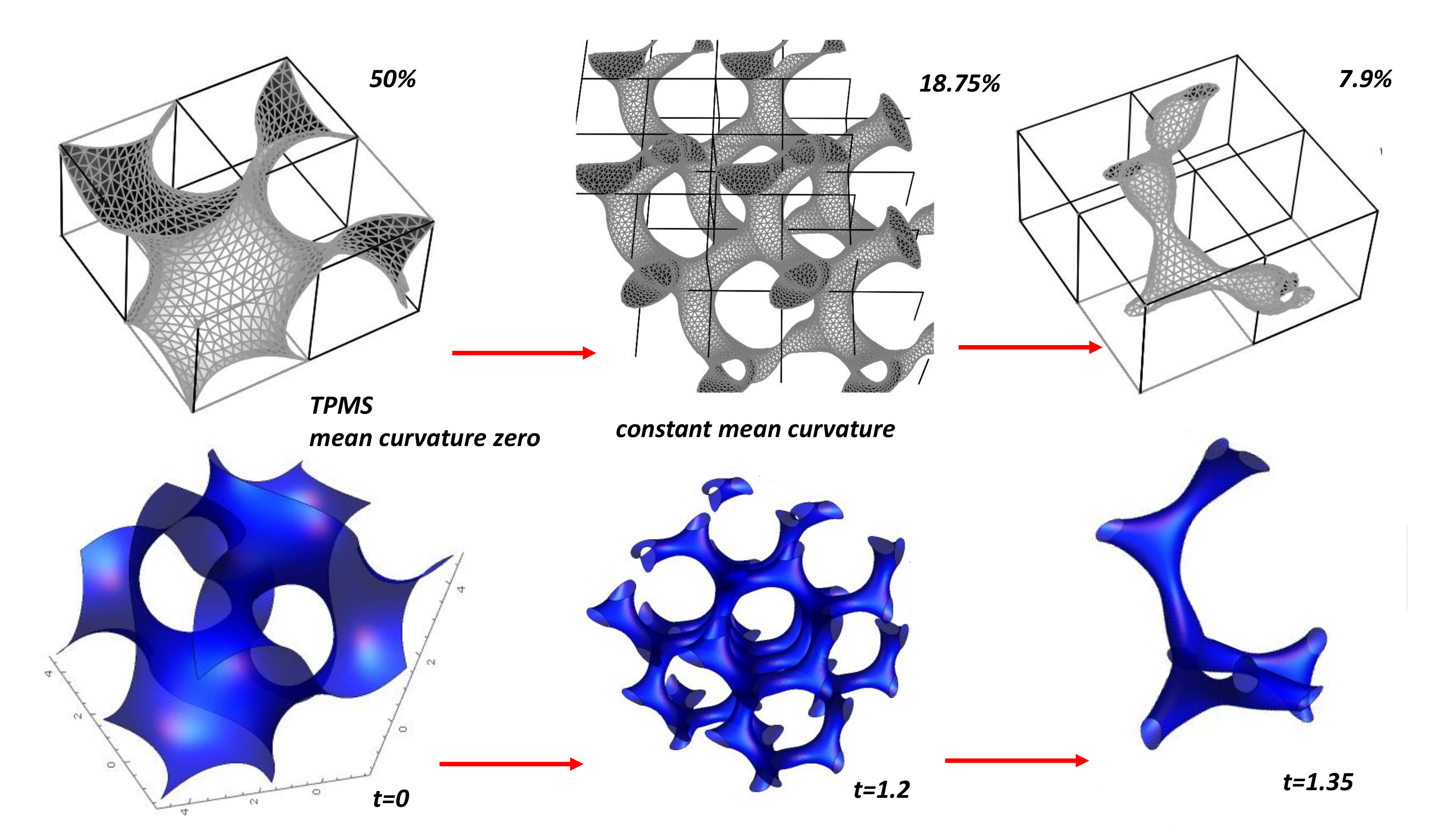
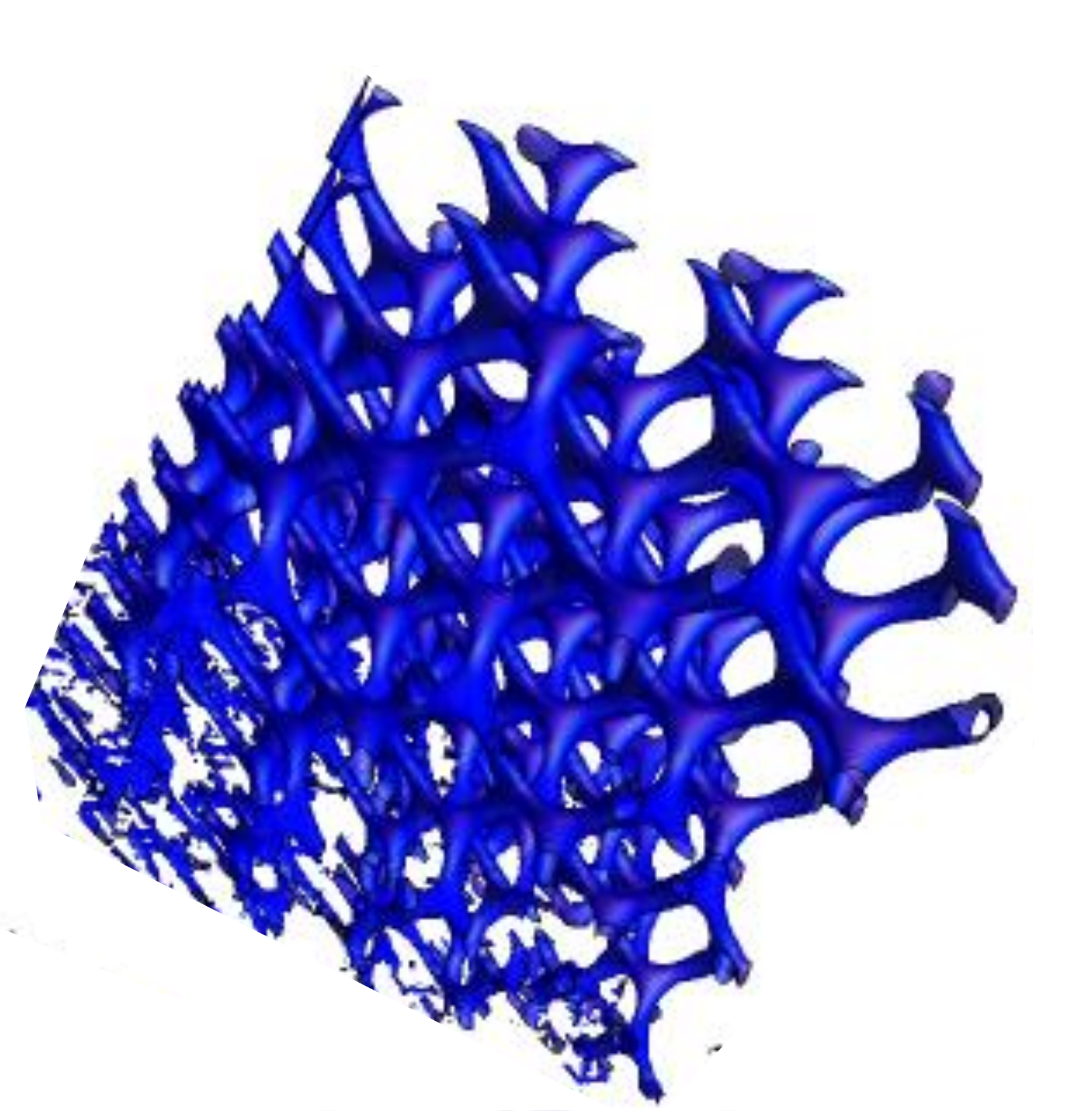
- The nanotubes with and , thus . The fourth belongs to the minimal surfaces, among them the triply periodic minimal surfaces (TPMS) with , . From a physical point of view TPMS are metastable structures. The excess in “strain” energy is evidenced after relaxation of a P-TPMS unit cell with boundaries [122] (Figure 27). Then, GLC cannot accommodate large holes that characterise giant Schwarzites (with a high number of hexagons) because of a complete relaxation. This is not the case for the smallest Schwarzites which are not smooth surfaces. Willmore energy states for smooth surfaces. One can define the discrete Willmore energy after tiling [145]. The physical stability is obtained minimising the discrete Willmore energy. We can discuss now the case of discrete surface in terms of local Euler characteristic.
5.7.2. Defect Formula: “Mathematical” Stability
5.7.3. “Physical” Stability
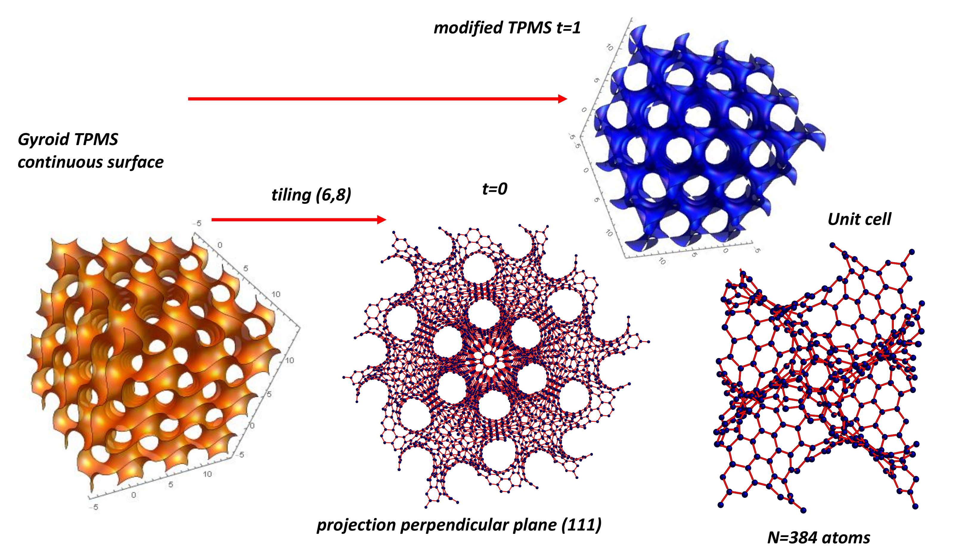
5.8. GLC Modeling from TPMS Structure
5.8.1. Constant Mean Curvature
5.8.2. Modified TPMS Structures: Strengths and Weaknesses
6. Conclusions
Funding
Institutional Review Board Statement
Informed Consent Statement
Data Availability Statement
Acknowledgments
Conflicts of Interest
Appendix A
References
- Gupta, S.; Saxena, A. The Role of Topology in Materials; Springer: Berlin/Heidelberg, Germany, 2018; Volume 189. [Google Scholar]
- Pesin, L. Review Structure and properties of glass-like carbon. J. Mater. Sci. 2002, 37, 1–28. [Google Scholar] [CrossRef]
- Zhang, J.; Ji, Y.; Dong, H.; Wang, W.; Chen, Z. Electrochemical determination of glucose using a platinum–palladium nanoparticle carbon nanofiber glassy carbon electrode. Anal. Lett. 2016, 49, 2741–2754. [Google Scholar] [CrossRef]
- Walsh, F.; Arenas, L.; de León, C.P.; Reade, G.; Whyte, I.; Mellor, B. The continued development of reticulated vitreous carbon as a versatile electrode material: Structure, properties and applications. Electrochim. Acta 2016, 215, 566–591. [Google Scholar] [CrossRef]
- Hoffmann, R.; Kabanov, A.A.; Golov, A.A.; Proserpio, D.M. Homo citans and carbon allotropes: For an ethics of citation. Angew. Chem. Int. Ed. 2016, 55, 10962–10976. [Google Scholar] [CrossRef]
- Suarez-Martinez, I.; Grobert, N.; Ewels, C. Nomenclature of sp2 carbon nanoforms. Carbon 2011, 50, 741–747. [Google Scholar] [CrossRef]
- Franklin, R.E. The interpretation of diffuse X-ray diagrams of carbon. Acta Crystallogr. 1950, 3, 107–121. [Google Scholar] [CrossRef]
- Harris, P.J.; Suarez-Martinez, I. Rosalind Franklin, carbon scientist. Carbon 2021, 171, 289–293. [Google Scholar] [CrossRef]
- Noda, T.; Inagaki, M. The structure of glassy carbon. Bull. Chem. Soc. Jpn. 1964, 37, 1534–1538. [Google Scholar] [CrossRef]
- Crawford, D.; Johnson, D. High-resolution electron microscopy of high-modulus carbon fibres. J. Microsc. 1971, 94, 51–62. [Google Scholar] [CrossRef]
- Ban, L.; Crawford, D.; Marsh, H. Lattice-resolution electron microscopy in structural studies of non-graphitizing carbons from polyvinylidene chloride (PVDC). J. Appl. Crystallogr. 1975, 8, 415–420. [Google Scholar] [CrossRef]
- Jenkins, G.; Kawamura, K. Structure of glassy carbon. Nature 1971, 231, 175. [Google Scholar] [CrossRef]
- Shiraishi, M. Kaitei Tansozairyo Nyumon (Introduction to Carbon Materials). Tanso Zair. Gakkai 1984, 29–33. [Google Scholar]
- Barborini, E.; Piseri, P.; Milani, P.; Benedek, G.; Ducati, C.; Robertson, J. Negatively curved spongy carbon. Appl. Phys. Lett. 2002, 81, 3359–3361. [Google Scholar] [CrossRef]
- Townsend, S.; Lenosky, T.; Muller, D.; Nichols, C.; Elser, V. Negatively curved graphitic sheet model of amorphous carbon. Phys. Rev. Lett. 1992, 69, 921. [Google Scholar] [CrossRef]
- Cataldo, F.; Graovac, A.; Ori, O. The Mathematics and Topology of Fullerenes; Springer Science & Business Media: Berlin/Heidelberg, Germany, 2011; Volume 4. [Google Scholar]
- Harris, P. Fullerene-related structure of commercial glassy carbons. Philos. Mag. 2004, 84, 3159–3167. [Google Scholar] [CrossRef]
- Jurkiewicz, K.; Duber, S.; Fischer, H.; Burian, A. Modelling of glass-like carbon structure and its experimental verification by neutron and X-ray diffraction. J. Appl. Crystallogr. 2017, 50, 36–48. [Google Scholar] [CrossRef]
- Acharya, M.; Strano, M.S.; Mathews, J.P.; Billinge, S.J.; Petkov, V.; Subramoney, S.; Foley, H.C. Simulation of nanoporous carbons: A chemically constrained structure. Philos. Mag. B 1999, 79, 1499–1518. [Google Scholar] [CrossRef]
- Shiell, T.B.; McCulloch, D.G.; McKenzie, D.R.; Field, M.; Haberl, B.; Boehler, R.; Cook, B.; De Tomas, C.; Suarez-Martinez, I.; Marks, N.; et al. Graphitization of glassy carbon after compression at room temperature. Phys. Rev. Lett. 2018, 120, 215701. [Google Scholar] [CrossRef]
- Benedek, G.; Vahedi-Tafreshi, H.; Barborini, E.; Piseri, P.; Milani, P.; Ducati, C.; Robertson, J. The structure of negatively curved spongy carbon. Diam. Relat. Mater. 2003, 12, 768–773. [Google Scholar] [CrossRef]
- Benedek, G.; Bernasconi, M.; Cinquanta, E.; D’Alessio, L.; De Corato, M. The topological background of schwarzite physics. In The Mathematics and Topology of Fullerenes; Springer: Berlin/Heidelberg, Germany, 2011; pp. 217–247. [Google Scholar]
- Kuc, A.; Seifert, G. Hexagon-preserving carbon foams: Properties of hypothetical carbon allotropes. Phys. Rev. B 2006, 74, 214104. [Google Scholar] [CrossRef]
- Shiell, T.B.; McCulloch, D.G.; Bradby, J.E.; Haberl, B.; McKenzie, D.R. Neutron diffraction discriminates between models for the nanoarchitecture of graphene sheets in glassy carbon. J. Non-Cryst. Solids 2021, 554, 120610. [Google Scholar] [CrossRef]
- Malard, L.; Pimenta, M.A.; Dresselhaus, G.; Dresselhaus, M. Raman spectroscopy in graphene. Phys. Rep. 2009, 473, 51–87. [Google Scholar] [CrossRef]
- Bukalov, S.; Leites, L.; Sorokin, A.; Kotosonov, A. Structural changes in industrial glassy carbon as a function of heat treatment temperature according to Raman spectroscopy and X-ray diffraction data. Nanosyst. Phys. Chem. Math. 2014, 5, 186–191. [Google Scholar]
- Pauly, N.; Novak, M.; Tougaard, S. Surface excitation parameter for allotropic forms of carbon. Surf. Interface Anal. 2013, 45, 811–816. [Google Scholar] [CrossRef]
- Suzuki, S.; Yoshimura, M. Chemical stability of graphene coated silver substrates for surface-enhanced Raman scattering. Sci. Rep. 2017, 7, 14851. [Google Scholar] [CrossRef]
- Saxena, R.R.; Bragg, R.H. Electrical conduction in glassy carbon. J. Non-Cryst. Solids 1978, 28, 45–60. [Google Scholar] [CrossRef][Green Version]
- Ferrer-Argemi, L.; Cisquella-Serra, A.; Madou, M.; Lee, J. Temperature-Dependent Electrical and Thermal Conductivity of Glassy Carbon Wires. In Proceedings of the 2018 17th IEEE Intersociety Conference on Thermal and Thermomechanical Phenomena in Electronic Systems (ITherm), San Diego, CA, USA, 29 May–1 June 2018; pp. 1280–1288. [Google Scholar]
- Vomero, M.; Castagnola, E.; Ciarpella, F.; Maggiolini, E.; Goshi, N.; Zucchini, E.; Carli, S.; Fadiga, L.; Kassegne, S.; Ricci, D. Highly stable glassy carbon interfaces for long-term neural stimulation and low-noise recording of brain activity. Sci. Rep. 2017, 7, 40332. [Google Scholar] [CrossRef] [PubMed]
- Soukup, L.; Gregora, I.; Jastrabik, L.; Koňáková, A. Raman spectra and electrical conductivity of glassy carbon. Mater. Sci. Eng. B 1992, 11, 355–357. [Google Scholar] [CrossRef]
- Ferrari, A.C.; Robertson, J. Interpretation of Raman spectra of disordered and amorphous carbon. Phys. Rev. B 2000, 61, 14095. [Google Scholar] [CrossRef]
- Antony, R.P.; Preethi, L.; Gupta, B.; Mathews, T.; Dash, S.; Tyagi, A. Efficient electrocatalytic performance of thermally exfoliated reduced graphene oxide-Pt hybrid. Mater. Res. Bull. 2015, 70, 60–67. [Google Scholar] [CrossRef]
- Tuinstra, F.; Koenig, J.L. Raman spectrum of graphite. J. Chem. Phys. 1970, 53, 1126–1130. [Google Scholar] [CrossRef]
- Ferrari, A.; Rodil, S.; Robertson, J. Interpretation of infrared and Raman spectra of amorphous carbon nitrides. Phys. Rev. B 2003, 67, 155306. [Google Scholar] [CrossRef]
- Harris, P.J.F. Structure of non-graphitising carbons. Int. Mater. Rev. 1997, 42, 206–218. [Google Scholar] [CrossRef]
- Zakhidov, A.A.; Baughman, R.H.; Iqbal, Z.; Cui, C.; Khayrullin, I.; Dantas, S.O.; Marti, J.; Ralchenko, V.G. Carbon structures with three-dimensional periodicity at optical wavelengths. Science 1998, 282, 897–901. [Google Scholar] [CrossRef]
- Pierini, F.; Lanzi, M.; Lesci, I.G.; Roveri, N. Comparison between inorganic geomimetic chrysotile and multiwalled carbon nanotubes in the preparation of one-dimensional conducting polymer nanocomposites. Fibers Polym. 2015, 16, 426–433. [Google Scholar] [CrossRef]
- Kaplas, T.; Svirko, Y.P. Direct deposition of semitransparent conducting pyrolytic carbon films. J. Nanophotonics 2012, 6, 061703. [Google Scholar] [CrossRef]
- López-Honorato, E.; Meadows, P.; Shatwell, R.; Xiao, P. Characterization of the anisotropy of pyrolytic carbon by Raman spectroscopy. Carbon 2010, 48, 881–890. [Google Scholar] [CrossRef]
- Harris, P.J.; Tsang, S.C.; Claridge, J.B.; Green, M.L. High-resolution electron microscopy studies of a microporous carbon produced by arc-evaporation. J. Chem. Soc. Faraday Trans. 1994, 90, 2799–2802. [Google Scholar] [CrossRef]
- Fogg, J.L.; Putman, K.J.; Zhang, T.; Lei, Y.; Terrones, M.; Harris, P.J.; Marks, N.A.; Suarez-Martinez, I. Catalysis-free transformation of non-graphitising carbons into highly crystalline graphite. Commun. Mater. 2020, 1, 47. [Google Scholar] [CrossRef]
- Zhang, L.; Zhang, F.; Yang, X.; Long, G.; Wu, Y.; Zhang, T.; Leng, K.; Huang, Y.; Ma, Y.; Yu, A.; et al. Porous 3D graphene-based bulk materials with exceptional high surface area and excellent conductivity for supercapacitors. Sci. Rep. 2013, 3, 1408. [Google Scholar] [CrossRef]
- Scheffler, M.; Colombo, P. Cellular Ceramics: Structure, Manufacturing, Properties and Applications; John Wiley & Sons: Hoboken, NJ, USA, 2006. [Google Scholar]
- Diaf, H.; Pereira, A.; Melinon, P.; Blanchard, N.; Bourquard, F.; Garrelie, F.; Donnet, C.; Vondráčk, M. Revisiting thin film of glassy carbon. Phys. Rev. Mater. 2020, 4, 066002. [Google Scholar] [CrossRef]
- Toh, C.T.; Zhang, H.; Lin, J.; Mayorov, A.S.; Wang, Y.P.; Orofeo, C.M.; Ferry, D.B.; Andersen, H.; Kakenov, N.; Guo, Z.; et al. Synthesis and properties of free-standing monolayer amorphous carbon. Nature 2020, 577, 199–203. [Google Scholar] [CrossRef]
- Xie, W.; Wei, Y. Roughening for Strengthening and Toughening in Monolayer Carbon Based Composites. Nano Lett. 2021. [Google Scholar] [CrossRef]
- Roy, D.; Chhowalla, M.; Wang, H.; Sano, N.; Alexandrou, I.; Clyne, T.; Amaratunga, G. Characterisation of carbon nano-onions using Raman spectroscopy. Chem. Phys. Lett. 2003, 373, 52–56. [Google Scholar] [CrossRef]
- Tan, P.; Dimovski, S.; Gogotsi, Y. Raman scattering of non–planar graphite: Arched edges, polyhedral crystals, whiskers and cones. Philos. Trans. R. Soc. Lond. Ser. A Math. Phys. Eng. Sci. 2004, 362, 2289–2310. [Google Scholar] [CrossRef]
- Castelvecchi, D. The shape of things to come. Nature 2017, 547, 272–274. [Google Scholar] [CrossRef]
- Kaye, A. Two-Dimensional Orbifolds 2007. Available online: https://math.uchicago.edu\T1\guilsinglrightFINALFULL\T1\guilsinglrightKaye (accessed on 15 May 2021).
- Gallier, J.; Xu, D. A Guide to the Classification Theorem for Compact Surfaces; Springer Science & Business Media: Berlin/Heidelberg, Germany, 2013. [Google Scholar]
- Haddon, R.; Brus, L.; Raghavachari, K. Rehybridization and π-orbital alignment: The key to the existence of spheroidal carbon clusters. Chem. Phys. Lett. 1986, 131, 165–169. [Google Scholar] [CrossRef]
- Available online: https://www.open.edu/openlearn/science-maths-technology/mathematics-statistics/surfaces/ (accessed on 15 May 2021).
- Spanier, E.H. Algebraic Topology; Springer Science & Business Media: Berlin/Heidelberg, Germany, 1989. [Google Scholar]
- Munkres, J.R. Elements of Algebraic Topology; CRC Press: Boca Raton, FL, USA, 2018. [Google Scholar]
- George, T. The Classification of Surfaces with Boundary 2011. Available online: http://www.math.uchicago.edu\T1\guilsinglrightVIGRE\T1\guilsinglrightGeorge (accessed on 15 May 2021).
- Zomorodian, A. Computational topology. Algorithms Theory Comput. Handb. 2009, 2, 3. [Google Scholar]
- Pranav, P.; Edelsbrunner, H.; Van de Weygaert, R.; Vegter, G.; Kerber, M.; Jones, B.J.; Wintraecken, M. The topology of the cosmic web in terms of persistent Betti numbers. Mon. Not. R. Astron. Soc. 2017, 465, 4281–4310. [Google Scholar] [CrossRef]
- Hitchin, N. Geometry of Surfaces; Lecture Notes B3; Springer Science & Business Media: Berlin/Heidelberg, Germany, 2004. [Google Scholar]
- Kinsey, L.C. Topology of Surfaces; Springer Science & Business Media: Berlin/Heidelberg, Germany, 1997. [Google Scholar]
- Zhang, H.J.; Chadov, S.; Müchler, L.; Yan, B.; Qi, X.L.; Kübler, J.; Zhang, S.C.; Felser, C. Topological insulators in ternary compounds with a honeycomb lattice. Phys. Rev. Lett. 2011, 106, 156402. [Google Scholar] [CrossRef]
- Moore, J.E. The birth of topological insulators. Nature 2010, 464, 194–198. [Google Scholar] [CrossRef]
- Franz, M.; Molenkamp, L. Topological Insulators; Elsevier: Amsterdam, The Netherlands, 2013. [Google Scholar]
- Lui, L.M.; Wen, C. Geometric registration of high-genus surfaces. SIAM J. Imaging Sci. 2014, 7, 337–365. [Google Scholar] [CrossRef][Green Version]
- Smith, W.; Mann, R.B. Formation of topological black holes from gravitational collapse. Phys. Rev. D 1997, 56, 4942. [Google Scholar] [CrossRef]
- Cayssol, J. Introduction to Dirac materials and topological insulators. Comptes Rendus Phys. 2013, 14, 760–778. [Google Scholar] [CrossRef]
- Khan, M.; Kamran, M.; Babar, S. On topological aspects of 2D graphene like materials. arXiv 2014, arXiv:1408.6124. [Google Scholar]
- Hyde, S.; Ramsden, S.; Robins, V. Unification and classification of two-dimensional crystalline patterns using orbifolds. Acta Crystallogr. Sect. A Found. Adv. 2014, 70, 319–337. [Google Scholar] [CrossRef]
- Rotskoff, G. The Gauss-Bonnet Theorem 2010. Available online: http://www.math.uchicago.edu/VIGRE/Rotskoff (accessed on 15 May 2021).
- Thurston, B. The orbifold notation for surface groups. Groups Comb. Geom. 1992, 165, 438. [Google Scholar]
- Conway, J.H.; Huson, D.H. The orbifold notation for two-dimensional groups. Struct. Chem. 2002, 13, 247–257. [Google Scholar] [CrossRef]
- Coxeter, H.S. Discrete groups generated by reflections. Ann. Math. 1934, 35, 588–621. [Google Scholar] [CrossRef]
- Kolbe, B.; Evans, M.E. Isotopic tiling theory for hyperbolic surfaces. Geom. Dedicata 2020, 21, 177–204. [Google Scholar] [CrossRef]
- Huson, D. Two-Dimensional Symmetry Mutation 1991. Available online: https://www.researchgate.net/publication/2422380_Two-Dimensional_Symmetry_Mutation (accessed on 15 May 2021).
- Schoen, A.H. Infinite Periodic Minimal Surfaces without Self-Intersections; National Aeronautics and Space Administration: Washington, DC, USA, 1970. [Google Scholar]
- Jung, Y.; Chu, K.T.; Torquato, S. A variational level set approach for surface area minimization of triply-periodic surfaces. J. Comput. Phys. 2007, 223, 711–730. [Google Scholar] [CrossRef][Green Version]
- Meeks, W.H., III. The theory of triply periodic minimal surfaces. Indiana Univ. Math. J. 1990, 39, 877–936. [Google Scholar] [CrossRef]
- Li, Y.; Guo, S. Triply periodic minimal surface using a modified Allen–Cahn equation. Appl. Math. Comput. 2017, 295, 84–94. [Google Scholar] [CrossRef]
- Gandy, P.J.; Klinowski, J. The equipotential surfaces of cubic lattices. Chem. Phys. Lett. 2002, 360, 543–551. [Google Scholar] [CrossRef]
- Mickel, W.; Schröder-Turk, G.E.; Mecke, K. Tensorial Minkowski functionals of triply periodic minimal surfaces. Interface Focus 2012, 2, 623–633. [Google Scholar] [CrossRef]
- Schoen, A.H. On the graph (10,3)-a. Not. Am. Math. Soc. 2008, 55, 663. [Google Scholar]
- Gandy, P.J.; Klinowski, J. Exact computation of the triply periodic G (Gyroid’) minimal surface. Chem. Phys. Lett. 2000, 321, 363–371. [Google Scholar] [CrossRef]
- Restrepo, S.; Ocampo, S.; Ramírez, J.; Paucar, C.; García, C. Mechanical properties of ceramic structures based on triply periodic minimal surface (TPMS) processed by 3D printing. J. Phys. Conf. Ser. 2017, 935, 012036. [Google Scholar] [CrossRef]
- King, R.B. Platonic tessellations of Riemann surfaces as models in chemistry: Non-zero genus analogues of regular polyhedra. J. Mol. Struct. 2003, 656, 119–133. [Google Scholar] [CrossRef]
- Terrones, H.; Terrones, M. Curved nanostructured materials. New J. Phys. 2003, 5, 126. [Google Scholar] [CrossRef]
- Karabáš, J.; Nedela, R. Archimedean maps of higher genera. Math. Comput. 2012, 81, 569–583. [Google Scholar] [CrossRef]
- Sadoc, J.; Charvolin, J. The crystallography of the hyperbolic plane and infinite periodic minimal surfaces. Le J. De Phys. Colloq. 1990, 51, C7-319–C7-332. [Google Scholar] [CrossRef]
- Robins, V.; Ramsden, S.; Hyde, S. 2D hyperbolic groups induce three-periodic Euclidean reticulations. Eur. Phys. J. B-Condens. Matter Complex Syst. 2004, 39, 365–375. [Google Scholar] [CrossRef]
- Ramsden, S.; Robins, V.; Hyde, S. Three-dimensional Euclidean nets from two-dimensional hyperbolic tilings: Kaleidoscopic examples. Acta Crystallogr. Sect. A Found. Crystallogr. 2009, 65, 81–108. [Google Scholar] [CrossRef]
- Lynch, M.L.; Spicer, P.T. Bicontinuous Liquid Crystals; CRC Press: Boca Raton, FL, USA, 2005; Volume 127. [Google Scholar]
- Mecke, K.R.; Stoyan, D. Morphology of Condensed Matter: Physics and Geometry of Spatially Complex Systems; Springer Science & Business Media: Berlin/Heidelberg, Germany, 2002; Volume 600. [Google Scholar]
- Park, S.; Kittimanapun, K.; Ahn, J.S.; Kwon, Y.K.; Tománek, D. Designing rigid carbon foams. J. Phys. Condens. Matter 2010, 22, 334220. [Google Scholar] [CrossRef]
- Owens, J.; Daniels, C.; Nicolaï, A.; Terrones, H.; Meunier, V. Structural, energetic, and electronic properties of gyroidal graphene nanostructures. Carbon 2016, 96, 998–1007. [Google Scholar] [CrossRef]
- Weng, H.; Liang, Y.; Xu, Q.; Yu, R.; Fang, Z.; Dai, X.; Kawazoe, Y. Topological node-line semimetal in three-dimensional graphene networks. Phys. Rev. B 2015, 92, 045108. [Google Scholar] [CrossRef]
- Herges, R. Topology in chemistry: Designing Möbius molecules. Chem. Rev. 2006, 106, 4820–4842. [Google Scholar] [CrossRef]
- Schaller, G.R.; Topić, F.; Rissanen, K.; Okamoto, Y.; Shen, J.; Herges, R. Design and synthesis of the first triply twisted Möbius annulene. Nat. Chem. 2014, 6, 608–613. [Google Scholar] [CrossRef]
- Schaller, G.R. Design und Synthese Moebius-Topologischer und Moebius-Aromatischer Kohlenwasserstoffe. Ph.D. Thesis, Christian-Albrechts Universität Kiel, Kiel, Germany, 2013. [Google Scholar]
- Henle, M. A Combinatorial Introduction to Topology; Dover Publications Inc: New York, NY, USA, 1994. [Google Scholar]
- Willard, S. General Topology; Courier Corporation: North Chelmsford, MA, USA, 2012. [Google Scholar]
- Yoon, K.; Rahnamoun, A.; Swett, J.L.; Iberi, V.; Cullen, D.A.; Vlassiouk, I.V.; Belianinov, A.; Jesse, S.; Sang, X.; Ovchinnikova, O.S.; et al. Atomistic-scale simulations of defect formation in graphene under noble gas ion irradiation. ACS Nano 2016, 10, 8376–8384. [Google Scholar] [CrossRef]
- Schubert, H. Die Eindeutige Zerlegbarkeit Eines Knotens in Primknoten; Springer: Berlin/Heidelberg, Germany, 2013. [Google Scholar]
- Fielden, S.D.; Leigh, D.A.; Woltering, S.L. Molecular knots. Angew. Chem. Int. Ed. 2017, 56, 11166–11194. [Google Scholar] [CrossRef]
- Scharein, R.G. Interactive Topological Drawing. Ph.D. Thesis, University of British Columbia, Vancouver, BC, Canada, 1998. [Google Scholar]
- Li, Q.; Ni, Z.; Gong, J.; Zhu, D.; Zhu, Z. Carbon nanotubes coated by carbon nanoparticles of turbostratic stacked graphenes. Carbon 2008, 46, 434–439. [Google Scholar] [CrossRef]
- Smajda, R.; Kukovecz, Á.; Kónya, Z.; Kiricsi, I. Structure and gas permeability of multi-wall carbon nanotube buckypapers. Carbon 2007, 45, 1176–1184. [Google Scholar] [CrossRef]
- Rolfsen, D. Knots and Links; American Mathematical Soc.: Providence, RI, USA, 2003; Volume 346. [Google Scholar]
- Marsh, G. J. Proc. Int. Symp. Carbon 1982, 81.
- Terrones, H.; Terrones, M.; Hernández, E.; Grobert, N.; Charlier, J.C.; Ajayan, P. New metallic allotropes of planar and tubular carbon. Phys. Rev. Lett. 2000, 84, 1716. [Google Scholar] [CrossRef]
- Rocquefelte, X.; Rignanese, G.M.; Meunier, V.; Terrones, H.; Terrones, M.; Charlier, J.C. How to identify Haeckelite structures: A theoretical study of their electronic and vibrational properties. Nano Lett. 2004, 4, 805–810. [Google Scholar] [CrossRef]
- Zhu, Z.; Fthenakis, Z.G.; Tománek, D. Electronic structure and transport in graphene/haeckelite hybrids: An ab initio study. 2D Materials 2015, 2, 035001. [Google Scholar] [CrossRef]
- Nisar, J.; Jiang, X.; Pathak, B.; Zhao, J.; Kang, T.W.; Ahuja, R. Semiconducting allotrope of graphene. Nanotechnology 2012, 23, 385704. [Google Scholar] [CrossRef]
- Sunada, T. Crystals that Nature Might MISS Creating; Notices Amer. Math. Soc.; Citeseer: Princeton, NJ, USA, 2008. [Google Scholar]
- Naito, H. A Short Lecture on Topological Crystallography and a Discrete Surface Theory. arXiv 2020, arXiv:2002.09562. [Google Scholar]
- Itoh, M.; Kotani, M.; Naito, H.; Sunada, T.; Kawazoe, Y.; Adschiri, T. New metallic carbon crystal. Phys. Rev. Lett. 2009, 102, 055703. [Google Scholar] [CrossRef]
- Dai, J.; Li, Z.; Yang, J. Boron K 4 crystal: A stable chiral three-dimensional sp 2 network. Phys. Chem. Chem. Phys. 2010, 12, 12420–12422. [Google Scholar] [CrossRef]
- Liu, J.; Zhang, S.; Guo, Y.; Wang, Q. Phosphorus K4 Crystal: A New Stable Allotrope. Sci. Rep. 2016, 6, 37528. [Google Scholar] [CrossRef]
- Zhong, C.; Xie, Y.; Chen, Y.; Zhang, S. Coexistence of flat bands and Dirac bands in a carbon-Kagome-lattice family. Carbon 2016, 99, 65–70. [Google Scholar] [CrossRef]
- Mott, P.; Roland, C. Limits to Poisson’s ratio in isotropic materials—General result for arbitrary deformation. Phys. Scr. 2013, 87, 055404. [Google Scholar] [CrossRef]
- Song, Y.; Qi, L.; Li, Y. Prediction of elastic properties of pyrolytic carbon based on orientation angle. In IOP Conference Series: Materials Science and Engineering; IOP Publishing: Bristol, UK, 2017; Volume 213, p. 012030. [Google Scholar]
- Miller, D.C.; Terrones, M.; Terrones, H. Mechanical properties of hypothetical graphene foams: Giant Schwarzites. Carbon 2016, 96, 1191–1199. [Google Scholar] [CrossRef]
- Garion, C. Mechanical properties for reliability analysis of structures in glassy carbon. World J. Mech. 2014, 4, 79–89. [Google Scholar] [CrossRef]
- Shiell, T.B.; Wong, S.; Yang, W.; Tanner, C.A.; Haberl, B.; Elliman, R.G.; McKenzie, D.R.; McCulloch, D.G.; Bradby, J.E. The composition, structure and properties of four different glassy carbons. J. Non-Cryst. Solids 2019, 522, 119561. [Google Scholar] [CrossRef]
- Manoharan, M.; Lee, H.; Rajagopalan, R.; Foley, H.; Haque, M. Elastic properties of 4–6 nm-thick glassy carbon thin films. Nanoscale Res. Lett. 2010, 5, 14–19. [Google Scholar] [CrossRef]
- Li, M.; Yuan, K.; Zhao, Y.; Gao, Z.; Zhao, X. A Novel Hyperbolic Two-Dimensional Carbon Material with an In-Plane Negative Poisson’s Ratio Behavior and Low-Gap Semiconductor Characteristics. ACS Omega 2020, 5, 15783–15790. [Google Scholar] [CrossRef]
- Kowalczyk, P.; Hołyst, R.; Terrones, M.; Terrones, H. Hydrogen storage in nanoporous carbon materials: Myth and facts. Phys. Chem. Chem. Phys. 2007, 9, 1786–1792. [Google Scholar] [CrossRef]
- Song, J.; Zhao, Y.; Zhang, W.; He, X.; Zhang, D.; He, Z.; Gao, Y.; Jin, C.; Xia, H.; Wang, J.; et al. Helium permeability of different structure pyrolytic carbon coatings on graphite prepared at low temperature and atmosphere pressure. J. Nucl. Mater. 2016, 468, 31–36. [Google Scholar] [CrossRef]
- Yamada, S.; Sato, H. Some physical properties of glassy carbon. Nature 1962, 193, 261–262. [Google Scholar] [CrossRef]
- Tomadakis, M.M.; Sotirchos, S.V. Ordinary and transition regime diffusion in random fiber structures. AIChE J. 1993, 39, 397–412. [Google Scholar] [CrossRef]
- Gostick, J.T.; Fowler, M.W.; Pritzker, M.D.; Ioannidis, M.A.; Behra, L.M. In-plane and through-plane gas permeability of carbon fiber electrode backing layers. J. Power Sources 2006, 162, 228–238. [Google Scholar] [CrossRef]
- Nicolaï, A.; Monti, J.; Daniels, C.; Meunier, V. Electrolyte Diffusion in Gyroidal Nanoporous Carbon. J. Phys. Chem. C 2015, 119, 2896–2903. [Google Scholar] [CrossRef]
- Furmaniak, S.; Gauden, P.; Terzyk, A.; Kowalczyk, P. Gyroidal nanoporous carbons-Adsorption and separation properties explored using computer simulations. arXiv 2016, arXiv:1603.02161. [Google Scholar] [CrossRef]
- Shimizu, R.; Tanaka, H. Impact of complex topology of porous media on phase separation of binary mixtures. Sci. Adv. 2017, 3, eaap9570. [Google Scholar] [CrossRef]
- Usseglio-Viretta, F.L.; Finegan, D.P.; Colclasure, A.; Heenan, T.M.; Abraham, D.; Shearing, P.; Smith, K. Quantitative relationships between pore tortuosity, pore topology, and solid particle morphology using a novel discrete particle size algorithm. J. Electrochem. Soc. 2020, 167, 100513. [Google Scholar] [CrossRef]
- Hormann, K.; Baranau, V.; Hlushkou, D.; Höltzel, A.; Tallarek, U. Topological analysis of non-granular, disordered porous media: Determination of pore connectivity, pore coordination, and geometric tortuosity in physically reconstructed silica monoliths. New J. Chem. 2016, 40, 4187–4199. [Google Scholar] [CrossRef]
- Haranczyk, M.; Sethian, J.A. Navigating molecular worms inside chemical labyrinths. Proc. Natl. Acad. Sci. USA 2009, 106, 21472–21477. [Google Scholar] [CrossRef]
- Nakashima, Y.; Kamiya, S. Mathematica programs for the analysis of three-dimensional pore connectivity and anisotropic tortuosity of porous rocks using X-ray computed tomography image data. J. Nucl. Sci. Technol. 2007, 44, 1233–1247. [Google Scholar] [CrossRef]
- Clennell, M.B. Tortuosity: A guide through the maze. Geol. Soc. Lond. Spec. Publ. 1997, 122, 299–344. [Google Scholar] [CrossRef]
- Ardayfio, C. Computational design of organic solar cell active layer through genetic algorithm. arXiv 2019, arXiv:1910.12401. [Google Scholar]
- Jiang, J.; Sandler, S.I. Separation of CO2 and N2 by adsorption in C168 schwarzite: A combination of quantum mechanics and molecular simulation study. J. Am. Chem. Soc. 2005, 127, 11989–11997. [Google Scholar] [CrossRef]
- Bryant, R.L. A duality theorem for Willmore surfaces. J. Differ. Geom. 1984, 20, 23–53. [Google Scholar] [CrossRef]
- Topping, P. Towards the Willmore conjecture. Calc. Var. Part. Differ. Equ. 2000, 11, 361–393. [Google Scholar] [CrossRef]
- Willmore, T.J. Note on Embedded Surfaces. 1965. Available online: https://www.math.uaic.ro/~annalsmath/pdf-uri%20anale/remarkable-papers/Thomas-J.-Willmore-1965.pdf (accessed on 15 May 2021).
- Bobenko, A.I. A conformal energy for simplicial surfaces. Comb. Comput. Geom. 2005, 52, 133–143. [Google Scholar]
- Hyde, S.; Ramsden, S.; Di Matteo, T.; Longdell, J. Ab-initio construction of some crystalline 3D Euclidean networks. Solid State Sci. 2003, 5, 35–45. [Google Scholar] [CrossRef]
- Hyde, S.; Ramsden, S. Some novel three-dimensional Euclidean crystalline networks derived from two-dimensional hyperbolic tilings. Eur. Phys. J. B-Condens. Matter Complex Syst. 2003, 31, 273–284. [Google Scholar] [CrossRef][Green Version]
- Wei, Y.; Wang, B.; Wu, J.; Yang, R.; Dunn, M.L. Bending rigidity and Gaussian bending stiffness of single-layered graphene. Nano Lett. 2012, 13, 26–30. [Google Scholar] [CrossRef]
- Yu, L.; Ru, C. Non-classical mechanical behavior of an elastic membrane with an independent Gaussian bending rigidity. Math. Mech. Solids 2017, 22, 491–501. [Google Scholar] [CrossRef]
- Koskinen, P.; Kit, O.O. Approximate modeling of spherical membranes. Phys. Rev. B 2010, 82, 235420. [Google Scholar] [CrossRef]
- Haddon, R. GVB and POAV analysis of rehybridization and π-orbital misalignment in non-planar conjugated systems. Chem. Phys. Lett. 1986, 125, 231–234. [Google Scholar] [CrossRef]
- Scott, L.T.; Bronstein, H.E.; Preda, D.V.; Ansems, R.B.; Bratcher, M.S.; Hagen, S. Geodesic polyarenes with exposed concave surfaces. Pure Appl. Chem. 1999, 71, 209–219. [Google Scholar] [CrossRef]
- Melinon, P.; Masenelli, B. From Small Fullerenes to Superlattices: Science and Applications; CRC Press: Boca Raton, FL, USA, 2012. [Google Scholar]
- Zhang, B.; Wang, C.; Ho, K.; Xu, C.; Chan, C.T. The geometry of small fullerene cages: C 20 to C 70. J. Chem. Phys. 1992, 97, 5007–5011. [Google Scholar] [CrossRef]
- Dunlap, B. Energetics and fullerene fractionation. Phys. Rev. B 1993, 47, 4018. [Google Scholar] [CrossRef]
- Große-Brauckmann, K. Gyroids of constant mean curvature. Exp. Math. 1997, 6, 33–50. [Google Scholar] [CrossRef]
- Grosse-Brauckmann, K. Triply periodic minimal and constant mean curvature surfaces. Interface Focus 2012, 2, 582–588. [Google Scholar] [CrossRef]
- Osserman, R. A Survey of Minimal Surfaces; Dover Publications, Inc.: Mineola, NY, USA, 2013. [Google Scholar]
- Tyson, J.T. Handout on Homeomorphisms, bi-Lipschitz Maps and Isometries. 2013. Available online: https://faculty.math.illinois.edu›~tyson›homeo (accessed on 15 May 2021).


| Allotrope | Peak cm | FWHM cm | Peak cm | FWHM cm | T Peak cm |
|---|---|---|---|---|---|
| graphene | 1582 ± 5 [25] | 13 | not relevant | not relevant | not relevant |
| GLC | 1585–1600 | 25–(70) | 1324–1329 [26] | 40–(100) | weak 1150 |
| Allotrope | Peak cm | Density | Porosity | Plasmon [27] eV | |
| graphene | asymmetric | not relevant | 2 | not relevant | 6.4 |
| GLC | symmetric | 1.2–1.5 g/cm | 3 | no | ∼6 |
| Allotrope | Graphitisation | Conductivity | Chemical Stability | ||
| graphene | yes | semi-metal-like | good [28] | ||
| GLC | no | complex [29,30] | very good [31] |
| Surface | g | |||
|---|---|---|---|---|
| sphere | 0 | 0 | 2 | 0 |
| n-fold torus | 0 | 0 | 2–2n | n |
| Klein bottle | 0 | 1 | 0 | |
| projective plane | 0 | 1 | 1 | |
| closed disc | 1 | 0 | 1 | |
| cylinder | 2 | 0 | 0 | 1 |
| Möbius band | 1 | 1 | 0 | 2 |
| closed orientable band | 2 | 0 | 0 | 1 |
| v | s | t | ||
|---|---|---|---|---|
| torus | 1 | −2 | 1 | 0 |
| sphere | 1 | 0 | 1 | 2 |
| Klein bottle | 1 | 1 | 0 | 0 |
| projective plan | 1 | 0 | 0 | 1 |
| Isometry | Orbifold Symbol | |
|---|---|---|
| (sphere) | 1 | 2 |
| pair of translations | o | -2 |
| rotation centre | A | (1-A)/A |
| reflection line | * | -1 |
| rotoreflection | (*) i | (1-i)/2i |
| glide line | x | -1 |
| Isometry | Orbifold Symbol | Group Number | |
|---|---|---|---|
| *632 | p6m | 17 | 0 |
| *333 | p3m1 | 14 | 0 |
| *442 | p4m | 11 | 0 |
| *2222 | pmm | 6 | 0 |
| Isometry | Orbifold Symbol | Group Number | |
|---|---|---|---|
| *235 | - | - | 1/60 |
| *234 | m3m | 221–230 | 1/24 |
| *233 | 3m | 215–220 | 1/12 |
| *22k | - | - | 1/2k |
| *226 | 6/mmm | 191–194 | 1/12 |
| *224 | 4/mmm | 123–142 | 1/8 |
| *223 | 2m | 189 | 1/6 |
| *222 | mmm | 47–74 | 1/4 |
| *kk | - | - | 1/k |
| *66 | 6mm | 183 | 1/6 |
| *44 | 4mm | 99–110 | 1/4 |
| *33 | 3m | 156–161 | 1/3 |
| *22 | mm2 | 25–46 | 1/2 |
| * | m | 6–9 | 1 |
| Orbifold Symbol | |
|---|---|
| *237 | −1/84 |
| *238 | −1/48 |
| *245 | −1/40 |
| *239 | −1/36 |
| *23 (10) | −1/30 |
| *23 (11) | −5/132 |
| *23 (12), *246, *334 | −1/24 |
| Name | Space Group | d in Å | N | x | y | z |
|---|---|---|---|---|---|---|
| D688 | 6.148 | 24 | 1:2 | 0.33342 | 0.66658 | |
| P688 | (229) | 7.828 | 48 | 0.31952 | 0.31952 | 0.09373 |
| G688 | 9.620 | 96 | 0.92205 | 0.12094 | 0.95502 | |
| gyroid | (230) | 18.599 | 384 | 0.18812 | 0.20968 | 0.77090 |
| 0.07632 | 0.20151 | 0.84364 | ||||
| 0.02066 | 0.15594 | 0.87348 |
Publisher’s Note: MDPI stays neutral with regard to jurisdictional claims in published maps and institutional affiliations. |
© 2021 by the author. Licensee MDPI, Basel, Switzerland. This article is an open access article distributed under the terms and conditions of the Creative Commons Attribution (CC BY) license (https://creativecommons.org/licenses/by/4.0/).
Share and Cite
Mélinon, P. Vitreous Carbon, Geometry and Topology: A Hollistic Approach. Nanomaterials 2021, 11, 1694. https://doi.org/10.3390/nano11071694
Mélinon P. Vitreous Carbon, Geometry and Topology: A Hollistic Approach. Nanomaterials. 2021; 11(7):1694. https://doi.org/10.3390/nano11071694
Chicago/Turabian StyleMélinon, Patrice. 2021. "Vitreous Carbon, Geometry and Topology: A Hollistic Approach" Nanomaterials 11, no. 7: 1694. https://doi.org/10.3390/nano11071694
APA StyleMélinon, P. (2021). Vitreous Carbon, Geometry and Topology: A Hollistic Approach. Nanomaterials, 11(7), 1694. https://doi.org/10.3390/nano11071694