Transcriptomics in Toxicogenomics, Part II: Preprocessing and Differential Expression Analysis for High Quality Data

 ,
,  , , , , ,
  , , , ,
  ,
,  ,
, 
Abstract
:
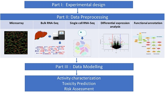
1. Introduction
2. Data Preprocessing
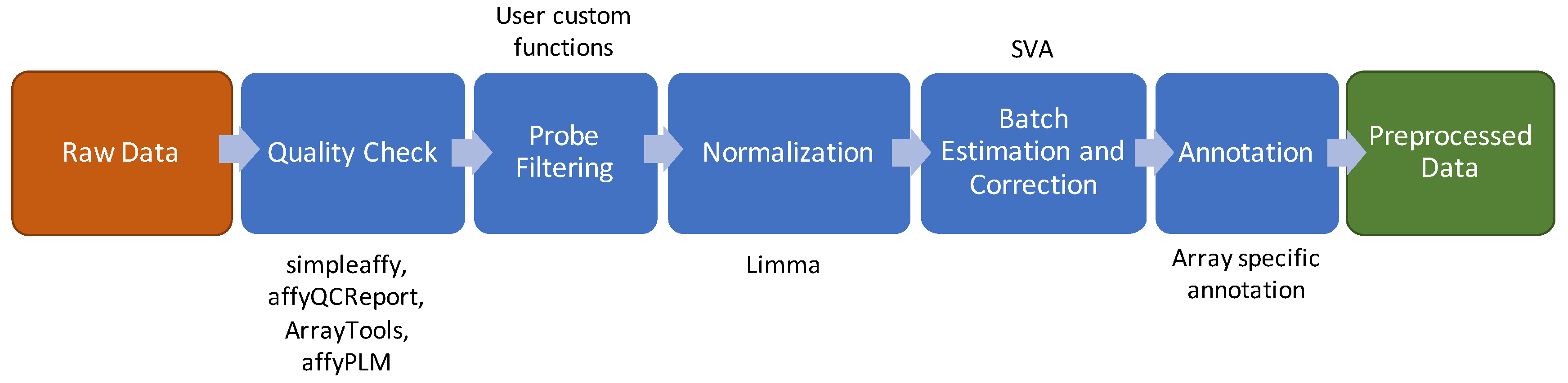
2.1. Microarray Experiments
2.2. Quality Check
2.3. Probe Prefiltering
2.4. Normalization
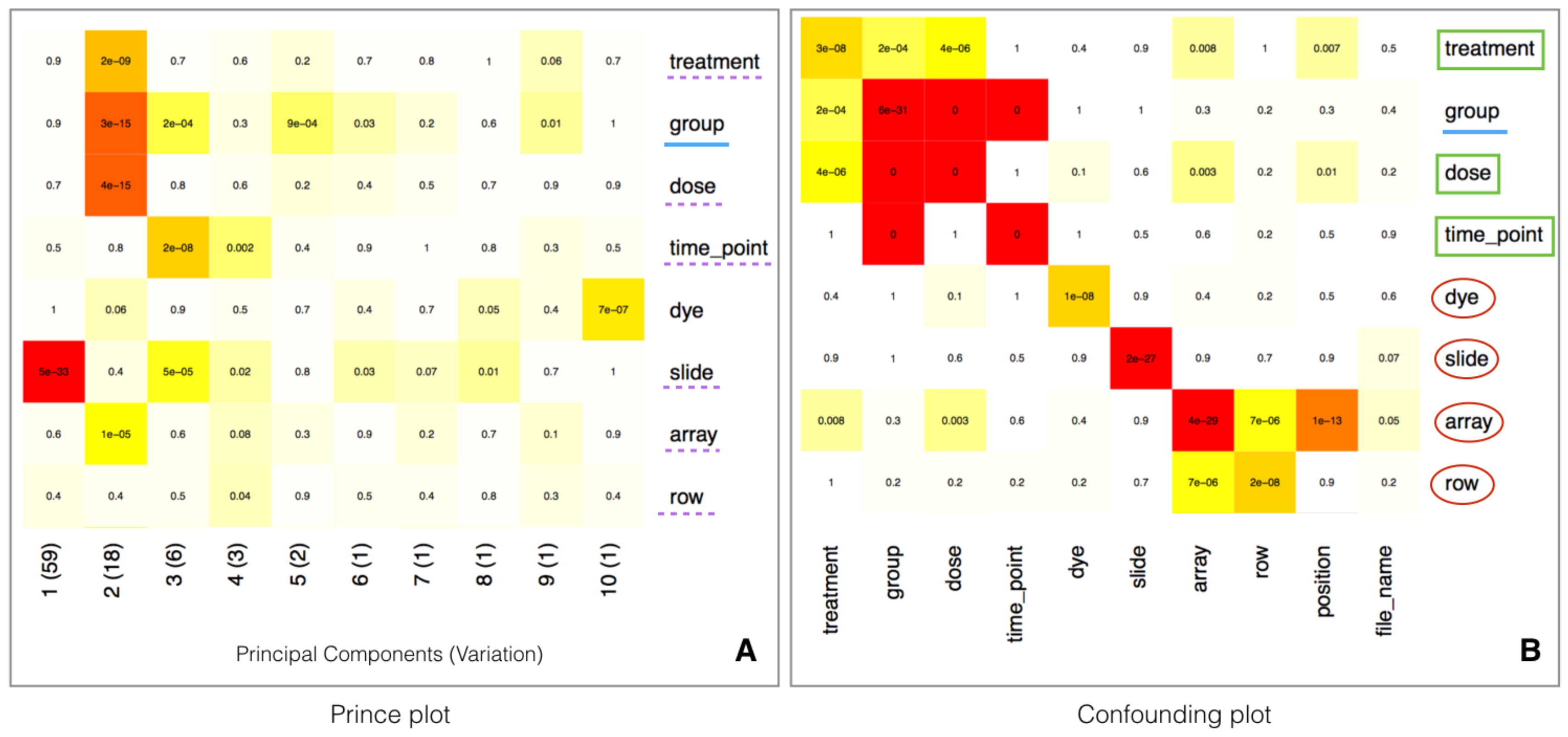
2.5. Batch Effect Estimation and Correction
2.6. Probe Annotation
2.7. Tools for Microarray Data Analysis
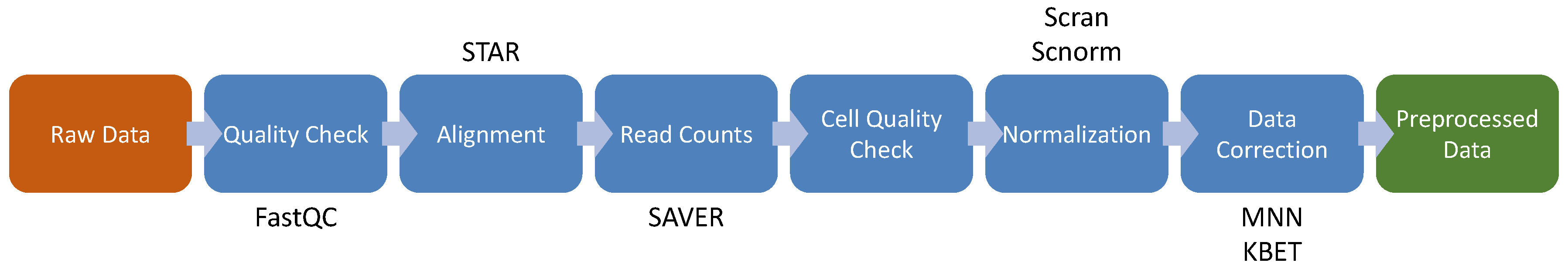
3. RNA Sequencing
3.1. Quality Check
3.2. Reads Alignment
3.3. Raw Counts Extraction
3.4. Normalization and Filtering
3.5. Batch Effect Estimation and Correction
4. Single Cell RNA-seq
4.1. Cell Quality Check
4.2. Feature Selection and Visualization
Cell Type Identification and Population Analysis
4.3. High-Throughput Transcriptomics
5. Differential Expression Analysis
6. Gene Functional Annotation and Pathway Analysis
7. Conclusions
Supplementary Materials
Author Contributions
Funding
Acknowledgments
Conflicts of Interest
Abbreviations
| AGA | Automated Genomics Analysis |
| BACA | Bubble Chart to Compare Biological Annotations |
| BWT | Burrow-Wheeler Transform |
| CAMERA | Correlation Adjusted MEan RAnk gene set test |
| CD | Cluster of Differentiation |
| CDF | Chip Description File |
| CEL-Seq | Cell Expression by Linear amplification and Sequencing |
| CMAP | Connectivity Map |
| DAVID | Database for Annotation, Visualization and Integrated Discovery |
| Drop-seq | Droplet sequencing |
| ENMs | Engineered Nanomaterials |
| eUTOPIA | solUTion for Omics data PreprocessIng and Analysis |
| FDR | False Discovery Rate |
| FPKM | Fragments Per Kilobase of exon model per Million mapped reads |
| FWER | Family-Wise Error Rate |
| GEO | Gene Expression Omnibus |
| GFM | Graph-based FM index |
| GLM | Generalized Linear Models |
| GO | Gene Ontology |
| GSEA | Gene Set Enrichment Analysis |
| HISAT2 | Hierarchical Indexing for Spliced Alignment of Transcripts 2 |
| HVGs | Highly Variable Genes |
| KBET | K-nearest neighbor Batch Effect Test |
| KEGG | Kyoto Encyclopedia of Genes and Genomes |
| L1000 | Library of Integrated Network-based Cellular Signatures 1000 |
| logCPM | log2-Counts Per Million |
| LOWESS | LOcally WEighted Scatterplot Smoothing |
| MARS-seq | MAssively parallel single-cell RNA-Sequencing |
| MeV | MultiExperiment Viewer |
| MNN | Mutual Nearest Neighbor |
| NCBI | National Center for Biotechnology Information |
| NGS | Next Generation Sequencing |
| Open TG-GATEs | ToxicoGenomics project-Genomics Assisted Toxicity Evaluation system |
| PCA | Principal Component Analysis |
| QC | Quality Check |
| RefSeq | Reference Sequence collection |
| RIN | RNA Integrity Number |
| RNA-seq | RNA sequencing |
| ROAST | ROtAtion Gene Set Tests |
| ROMER | ROtation testing using MEan Ranks |
| RPKM | Reads Per Kilobase of exon model per Million mapped reads |
| RSEM | RNA-Seq by Expectation Maximization |
| SAVER | Single-cell Analysis Via Expression Recovery |
| scRNA-seq | single cell RNA sequencing |
| SEQC | Sequence Quality Control |
| SVA | Surrogate Variable Analysis |
| SVM | Support Vector Machine |
| TGx | ToxicoGenomics |
| t-SNE | t-distributed Stochastic Neighbor Embedding |
| UMAP | Uniform Manifold Approximation and Projection |
| UMI | Unique Molecular Identifiers |
| UQUA | Upper Quantile |
References
- Waters, M.D.; Fostel, J.M. Toxicogenomics and systems toxicology: Aims and prospects. Nat. Rev. Genet. 2004, 5, 936–948. [Google Scholar] [CrossRef]
- Alexander-Dann, B.; Pruteanu, L.L.; Oerton, E.; Sharma, N.; Berindan-Neagoe, I.; Módos, D.; Bender, A. Developments in toxicogenomics: Understanding and predicting compound-induced toxicity from gene expression data. Mol. Omics 2018, 14, 218–236. [Google Scholar] [CrossRef] [PubMed] [Green Version]
- Casamassimi, A.; Federico, A.; Rienzo, M.; Esposito, S.; Ciccodicola, A. Transcriptome profiling in human diseases: New advances and perspectives. Int. J. Mol. Sci. 2017, 18, 1652. [Google Scholar] [CrossRef] [PubMed] [Green Version]
- Lamb, J. The Connectivity Map: A new tool for biomedical research. Nat. Rev. Cancer 2007, 7, 54–60. [Google Scholar] [CrossRef] [PubMed]
- Subramanian, A.; Narayan, R.; Corsello, S.M.; Peck, D.D.; Natoli, T.E.; Lu, X.; Gould, J.; Davis, J.F.; Tubelli, A.A.; Asiedu, J.K.; et al. A next generation connectivity map: L1000 platform and the first 1,000,000 profiles. Cell 2017, 171, 1437–1452. [Google Scholar] [CrossRef] [PubMed]
- Ganter, B.; Snyder, R.D.; Halbert, D.N.; Lee, M.D. Toxicogenomics in drug discovery and development: Mechanistic analysis of compound/class-dependent effects using the DrugMatrix® database. Future Med. 2006, 7. [Google Scholar] [CrossRef]
- Igarashi, Y.; Nakatsu, N.; Yamashita, T.; Ono, A.; Ohno, Y.; Urushidani, T.; Yamada, H. Open TG-GATEs: A large-scale toxicogenomics database. Nucleic Acids Res. 2015, 43, D921–D927. [Google Scholar] [CrossRef]
- Kolesnikov, N.; Hastings, E.; Keays, M.; Melnichuk, O.; Tang, Y.A.; Williams, E.; Dylag, M.; Kurbatova, N.; Brandizi, M.; Burdett, T.; et al. ArrayExpress update—Simplifying data submissions. Nucleic Acids Res. 2015, 43, D1113–D1116. [Google Scholar] [CrossRef]
- Edgar, R.; Domrachev, M.; Lash, A.E. Gene Expression Omnibus: NCBI gene expression and hybridization array data repository. Nucleic Acids Res. 2002, 30, 207–210. [Google Scholar] [CrossRef] [Green Version]
- Conesa, A.; Madrigal, P.; Tarazona, S.; Gomez-Cabrero, D.; Cervera, A.; McPherson, A.; Szcześniak, M.W.; Gaffney, D.J.; Elo, L.L.; Zhang, X.; et al. A survey of best practices for RNA-seq data analysis. Genome Biol. 2016, 17, 13. [Google Scholar] [CrossRef] [Green Version]
- Oshlack, A.; Robinson, M.D.; Young, M.D. From RNA-seq reads to differential expression results. Genome Biol. 2010, 11, 220. [Google Scholar] [CrossRef] [PubMed] [Green Version]
- Witten, D.M.; Tibshirani, R. Scientific research in the age of omics: The good, the bad, and the sloppy. J. Am. Med. Inform. Assoc. 2013, 20, 125–127. [Google Scholar] [CrossRef] [PubMed] [Green Version]
- Russo, F.; Righelli, D.; Angelini, C. Advantages and limits in the adoption of reproducible research and R-tools for the analysis of omic data. In International Meeting on Computational Intelligence Methods for Bioinformatics and Biostatistics; Springer: Berlin/Heidelberg, Germany, 2015; pp. 245–258. [Google Scholar]
- Quackenbush, J. Microarray data normalization and transformation. Nat. Genet. 2002, 32, 496–501. [Google Scholar] [CrossRef] [PubMed]
- Allison, D.B.; Cui, X.; Page, G.P.; Sabripour, M. Microarray data analysis: From disarray to consolidation and consensus. Nat. Rev. Genet. 2006, 7, 55–65. [Google Scholar] [CrossRef] [PubMed]
- Lee, E.K.; Park, T. Exploratory methods for checking quality of microarray data. Bioinformation 2007, 1, 423. [Google Scholar] [CrossRef] [PubMed] [Green Version]
- Bolstad, B.M.; Collin, F.; Simpson, K.M.; Irizarry, R.A.; Speed, T.P. Experimental design and low-level analysis of microarray data. Int. Rev. Neurobiol. 2004, 60, 25–58. [Google Scholar]
- Fasold, M.; Binder, H. AffyRNADegradation: Control and correction of RNA quality effects in GeneChip expression data. Bioinformatics 2013, 29, 129–131. [Google Scholar] [CrossRef] [Green Version]
- Eijssen, L.M.; Jaillard, M.; Adriaens, M.E.; Gaj, S.; de Groot, P.J.; Müller, M.; Evelo, C.T. User-friendly solutions for microarray quality control and pre-processing on ArrayAnalysis. org. Nucleic Acids Res. 2013, 41, W71–W76. [Google Scholar] [CrossRef] [Green Version]
- Gavin, A.J.S. Investigating the Mechanisms of Silver Nanoparticle Toxicity in Daphnia Magna: A Multi-Omics Approach. Ph.D. Thesis, University of Birmingham, Birmingham, UK, 2016. [Google Scholar]
- Yang, Y.H.; Dudoit, S.; Luu, P.; Lin, D.M.; Peng, V.; Ngai, J.; Speed, T.P. Normalization for cDNA microarray data: A robust composite method addressing single and multiple slide systematic variation. Nucleic Acids Res. 2002, 30, e15. [Google Scholar] [CrossRef] [Green Version]
- Bilban, M.; Buehler, L.K.; Head, S.; Desoye, G.; Quaranta, V. Normalizing DNA microarray data. Curr. Issues Mol. Biol. 2002, 4, 57–64. [Google Scholar]
- Yang, Y.H.; Dudoit, S.; Luu, P.; Speed, T.P. Normalization for cDNA microarry data. In Microarrays: Optical Technologies and Informatics; International Society for Optics and Photonics: Bellingham, WA, USA, 2001; Volume 4266, pp. 141–152. [Google Scholar]
- Cleveland, W.S. Robust locally weighted regression and smoothing scatterplots. J. Am. Stat. Assoc. 1979, 74, 829–836. [Google Scholar] [CrossRef]
- Hicks, S.C.; Irizarry, R.A. Quantro: A data-driven approach to guide the choice of an appropriate normalization method. Genome Biol. 2015, 16, 117. [Google Scholar] [CrossRef] [PubMed] [Green Version]
- Irizarry, R.A.; Bolstad, B.M.; Collin, F.; Cope, L.M.; Hobbs, B.; Speed, T.P. Summaries of Affymetrix GeneChip probe level data. Nucleic Acids Res. 2003, 31, e15. [Google Scholar] [CrossRef]
- Kupfer, P.; Guthke, R.; Pohlers, D.; Huber, R.; Koczan, D.; Kinne, R.W. Batch correction of microarray data substantially improves the identification of genes differentially expressed in rheumatoid arthritis and osteoarthritis. BMC Med. Genom. 2012, 5, 23. [Google Scholar] [CrossRef] [Green Version]
- Lazar, C.; Meganck, S.; Taminau, J.; Steenhoff, D.; Coletta, A.; Molter, C.; Weiss-Solís, D.Y.; Duque, R.; Bersini, H.; Nowé, A. Batch effect removal methods for microarray gene expression data integration: A survey. Briefings Bioinform. 2013, 14, 469–490. [Google Scholar] [CrossRef] [Green Version]
- Leek, J.T.; Johnson, W.E.; Parker, H.S.; Jaffe, A.E.; Storey, J.D. The sva package for removing batch effects and other unwanted variation in high-throughput experiments. Bioinformatics 2012, 28, 882–883. [Google Scholar] [CrossRef]
- Leek, J.T.; Scharpf, R.B.; Bravo, H.C.; Simcha, D.; Langmead, B.; Johnson, W.E.; Geman, D.; Baggerly, K.; Irizarry, R.A. Tackling the widespread and critical impact of batch effects in high-throughput data. Nat. Rev. Genet. 2010, 11, 733–739. [Google Scholar] [CrossRef] [Green Version]
- Johnson, W.E.; Li, C.; Rabinovic, A. Adjusting batch effects in microarray expression data using empirical Bayes methods. Biostatistics 2007, 8, 118–127. [Google Scholar] [CrossRef]
- Ritchie, M.E.; Phipson, B.; Wu, D.; Hu, Y.; Law, C.W.; Shi, W.; Smyth, G.K. limma powers differential expression analyses for RNA-sequencing and microarray studies. Nucleic Acids Res. 2015, 43, e47. [Google Scholar] [CrossRef]
- Arloth, J.; Bader, D.M.; Röh, S.; Altmann, A. Re-Annotator: Annotation pipeline for microarray probe sequences. PLoS ONE 2015, 10, e0139516. [Google Scholar] [CrossRef]
- Huber, W.; Carey, V.J.; Gentleman, R.; Anders, S.; Carlson, M.; Carvalho, B.S.; Bravo, H.C.; Davis, S.; Gatto, L.; Girke, T.; et al. Orchestrating high-throughput genomic analysis with Bioconductor. Nat. Methods 2015, 12, 115. [Google Scholar] [CrossRef] [PubMed]
- Considine, M.; Parker, H.; Wei, Y.; Xia, X.; Cope, L.; Ochs, M.; Fertig, E. AGA: Interactive pipeline for reproducible gene expression and DNA methylation data analyses. F1000Research 2015, 4, 28. [Google Scholar] [CrossRef] [PubMed]
- Howe, E.A.; Sinha, R.; Schlauch, D.; Quackenbush, J. RNA-Seq analysis in MeV. Bioinformatics 2011, 27, 3209–3210. [Google Scholar] [CrossRef] [PubMed] [Green Version]
- Cutts, R.J.; Dayem Ullah, A.Z.; Sangaralingam, A.; Gadaleta, E.; Lemoine, N.R.; Chelala, C. O-miner: An integrative platform for automated analysis and mining of-omics data. Nucleic Acids Res. 2012, 40, W560–W568. [Google Scholar] [CrossRef] [PubMed] [Green Version]
- Kallio, M.A.; Tuimala, J.T.; Hupponen, T.; Klemelä, P.; Gentile, M.; Scheinin, I.; Koski, M.; Käki, J.; Korpelainen, E.I. Chipster: User-friendly analysis software for microarray and other high-throughput data. BMC Genom. 2011, 12, 507. [Google Scholar] [CrossRef] [Green Version]
- Alonso, R.; Salavert, F.; Garcia-Garcia, F.; Carbonell-Caballero, J.; Bleda, M.; Garcia-Alonso, L.; Sanchis-Juan, A.; Perez-Gil, D.; Marin-Garcia, P.; Sanchez, R.; et al. Babelomics 5.0: Functional interpretation for new generations of genomic data. Nucleic Acids Res. 2015, 43, W117–W121. [Google Scholar] [CrossRef] [Green Version]
- Marwah, V.S.; Scala, G.; Kinaret, P.A.S.; Serra, A.; Alenius, H.; Fortino, V.; Greco, D. eUTOPIA: solUTion for Omics data PreprocessIng and Analysis. Source Code Biol. Med. 2019, 14, 1. [Google Scholar] [CrossRef] [Green Version]
- Auer, H.; Lyianarachchi, S.; Newsom, D.; Klisovic, M.I.; Marcucci, G.; Marcucci, U.; Kornacker, K. Chipping away at the chip bias: RNA degradation in microarray analysis. Nat. Genet. 2003, 35, 292–293. [Google Scholar] [CrossRef]
- Schroeder, A.; Mueller, O.; Stocker, S.; Salowsky, R.; Leiber, M.; Gassmann, M.; Lightfoot, S.; Menzel, W.; Granzow, M.; Ragg, T. The RIN: An RNA integrity number for assigning integrity values to RNA measurements. BMC Mol. Biol. 2006, 7, 3. [Google Scholar] [CrossRef] [Green Version]
- Gallego Romero, I.; Pai, A.A.; Tung, J.; Gilad, Y. RNA-seq: Impact of RNA degradation on transcript quantification. BMC Biol. 2014, 12, 42. [Google Scholar] [CrossRef] [Green Version]
- Ewing, B.; Green, P. Base-calling of automated sequencer traces using phred. II. Error probabilities. Genome Res. 1998, 8, 186–194. [Google Scholar] [CrossRef] [PubMed] [Green Version]
- Martin, M. Cutadapt removes adapter sequences from high-throughput sequencing reads. EMBnet. J. 2011, 17, 10–12. [Google Scholar] [CrossRef]
- Trapnell, C.; Pachter, L.; Salzberg, S.L. TopHat: Discovering splice junctions with RNA-Seq. Bioinformatics 2009, 25, 1105–1111. [Google Scholar] [CrossRef] [PubMed]
- Ameur, A.; Wetterbom, A.; Feuk, L.; Gyllensten, U. Global and unbiased detection of splice junctions from RNA-seq data. Genome Biol. 2010, 11, R34. [Google Scholar] [CrossRef] [Green Version]
- Kim, D.; Pertea, G.; Trapnell, C.; Pimentel, H.; Kelley, R.; Salzberg, S.L. TopHat2: Accurate alignment of transcriptomes in the presence of insertions, deletions and gene fusions. Genome Biol. 2013, 14, R36. [Google Scholar] [CrossRef] [Green Version]
- Pertea, M.; Kim, D.; Pertea, G.M.; Leek, J.T.; Salzberg, S.L. Transcript-level expression analysis of RNA-seq experiments with HISAT, StringTie and Ballgown. Nat. Protoc. 2016, 11, 1650. [Google Scholar] [CrossRef]
- Roberts, A.; Pimentel, H.; Trapnell, C.; Pachter, L. Identification of novel transcripts in annotated genomes using RNA-Seq. Bioinformatics 2011, 27, 2325–2329. [Google Scholar] [CrossRef]
- Pruitt, K.D.; Tatusova, T.; Maglott, D.R. NCBI reference sequences (RefSeq): A curated non-redundant sequence database of genomes, transcripts and proteins. Nucleic Acids Res. 2007, 35, D61–D65. [Google Scholar] [CrossRef] [Green Version]
- Wilming, L.G.; Gilbert, J.G.; Howe, K.; Trevanion, S.; Hubbard, T.; Harrow, J.L. The vertebrate genome annotation (Vega) database. Nucleic Acids Res. 2007, 36, D753–D760. [Google Scholar] [CrossRef] [Green Version]
- Liao, Y.; Smyth, G.K.; Shi, W. The R package Rsubread is easier, faster, cheaper and better for alignment and quantification of RNA sequencing reads. Nucleic Acids Res. 2019, 47, e47. [Google Scholar] [CrossRef] [Green Version]
- Anders, S.; Pyl, P.T.; Huber, W. HTSeq—A Python framework to work with high-throughput sequencing data. Bioinformatics 2015, 31, 166–169. [Google Scholar] [CrossRef] [PubMed]
- Mortazavi, A.; Williams, B.A.; McCue, K.; Schaeffer, L.; Wold, B. Mapping and quantifying mammalian transcriptomes by RNA-Seq. Nat. Methods 2008, 5, 621. [Google Scholar] [CrossRef] [PubMed]
- Evans, C.; Hardin, J.; Stoebel, D.M. Selecting between-sample RNA-Seq normalization methods from the perspective of their assumptions. Briefings Bioinform. 2018, 19, 776–792. [Google Scholar] [CrossRef] [PubMed]
- Bullard, J.H.; Purdom, E.; Hansen, K.D.; Dudoit, S. Evaluation of statistical methods for normalization and differential expression in mRNA-Seq experiments. BMC Bioinform. 2010, 11, 94. [Google Scholar] [CrossRef] [Green Version]
- Bourgon, R.; Gentleman, R.; Huber, W. Independent filtering increases detection power for high-throughput experiments. Proc. Natl. Acad. Sci. USA 2010, 107, 9546–9551. [Google Scholar] [CrossRef] [Green Version]
- Robinson, M.D.; McCarthy, D.J.; Smyth, G.K. edgeR: A Bioconductor package for differential expression analysis of digital gene expression data. Bioinformatics 2010, 26, 139–140. [Google Scholar] [CrossRef] [Green Version]
- Love, M.I.; Huber, W.; Anders, S. Moderated estimation of fold change and dispersion for RNA-seq data with DESeq2. Genome Biol. 2014, 15, 550. [Google Scholar] [CrossRef] [Green Version]
- Risso, D.; Ngai, J.; Speed, T.P.; Dudoit, S. Normalization of RNA-seq data using factor analysis of control genes or samples. Nat. Biotechnol. 2014, 32, 896. [Google Scholar] [CrossRef] [Green Version]
- Gagnon-Bartsch, J.A.; Speed, T.P. Using control genes to correct for unwanted variation in microarray data. Biostatistics 2012, 13, 539–552. [Google Scholar] [CrossRef] [Green Version]
- Jacob, L.; Gagnon-Bartsch, J.A.; Speed, T.P. Correcting gene expression data when neither the unwanted variation nor the factor of interest are observed. Biostatistics 2016, 17, 16–28. [Google Scholar] [CrossRef] [Green Version]
- Gagnon-Bartsch, J.A.; Jacob, L.; Speed, T.P. Removing Unwanted Variation from High Dimensional Data with Negative Controls; Technical Report; Department of Statistics, University of California: Berkeley, CA, USA, 2013; pp. 1–112. [Google Scholar]
- Tang, F.; Barbacioru, C.; Wang, Y.; Nordman, E.; Lee, C.; Xu, N.; Wang, X.; Bodeau, J.; Tuch, B.B.; Siddiqui, A.; et al. mRNA-Seq whole-transcriptome analysis of a single cell. Nat. Methods 2009, 6, 377. [Google Scholar] [CrossRef] [PubMed]
- Rostom, R.; Svensson, V.; Teichmann, S.A.; Kar, G. Computational approaches for interpreting scRNA-seq data. FEBS Lett. 2017, 591, 2213–2225. [Google Scholar] [CrossRef] [Green Version]
- Zappia, L.; Phipson, B.; Oshlack, A. Exploring the single-cell RNA-seq analysis landscape with the scRNA-tools database. PLoS Comput. Biol. 2018, 14, e1006245. [Google Scholar] [CrossRef] [PubMed]
- Zheng, G.X.; Terry, J.M.; Belgrader, P.; Ryvkin, P.; Bent, Z.W.; Wilson, R.; Ziraldo, S.B.; Wheeler, T.D.; McDermott, G.P.; Zhu, J.; et al. Massively parallel digital transcriptional profiling of single cells. Nat. Commun. 2017, 8, 1–12. [Google Scholar] [CrossRef] [Green Version]
- Klein, A.M.; Mazutis, L.; Akartuna, I.; Tallapragada, N.; Veres, A.; Li, V.; Peshkin, L.; Weitz, D.A.; Kirschner, M.W. Droplet barcoding for single-cell transcriptomics applied to embryonic stem cells. Cell 2015, 161, 1187–1201. [Google Scholar] [CrossRef] [Green Version]
- Azizi, E.; Carr, A.J.; Plitas, G.; Cornish, A.E.; Konopacki, C.; Prabhakaran, S.; Nainys, J.; Wu, K.; Kiseliovas, V.; Setty, M.; et al. Single-cell map of diverse immune phenotypes in the breast tumor microenvironment. Cell 2018, 174, 1293–1308. [Google Scholar] [CrossRef] [Green Version]
- Parekh, S.; Ziegenhain, C.; Vieth, B.; Enard, W.; Hellmann, I. zUMIs-a fast and flexible pipeline to process RNA sequencing data with UMIs. Gigascience 2018, 7, giy059. [Google Scholar] [CrossRef] [Green Version]
- Bacher, R.; Chu, L.F.; Leng, N.; Gasch, A.P.; Thomson, J.A.; Stewart, R.M.; Newton, M.; Kendziorski, C. SCnorm: Robust normalization of single-cell RNA-seq data. Nat. Methods 2017, 14, 584. [Google Scholar] [CrossRef] [Green Version]
- Lun, A.T.; Bach, K.; Marioni, J.C. Pooling across cells to normalize single-cell RNA sequencing data with many zero counts. Genome Biol. 2016, 17, 75. [Google Scholar] [CrossRef]
- Büttner, M.; Miao, Z.; Wolf, F.A.; Teichmann, S.A.; Theis, F.J. A test metric for assessing single-cell RNA-seq batch correction. Nat. Methods 2019, 16, 43–49. [Google Scholar] [CrossRef] [Green Version]
- Ilicic, T.; Kim, J.K.; Kolodziejczyk, A.A.; Bagger, F.O.; McCarthy, D.J.; Marioni, J.C.; Teichmann, S.A. Classification of low quality cells from single-cell RNA-seq data. Genome Biol. 2016, 17, 29. [Google Scholar] [CrossRef] [Green Version]
- Griffiths, J.A.; Scialdone, A.; Marioni, J.C. Using single-cell genomics to understand developmental processes and cell fate decisions. Mol. Syst. Biol. 2018, 14, e8046. [Google Scholar] [CrossRef] [PubMed]
- McGinnis, C.S.; Murrow, L.M.; Gartner, Z.J. DoubletFinder: Doublet detection in single-cell RNA sequencing data using artificial nearest neighbors. Cell Syst. 2019, 8, 329–337. [Google Scholar] [CrossRef] [PubMed]
- Luecken, M.D.; Theis, F.J. Current best practices in single-cell RNA-seq analysis: A tutorial. Mol. Syst. Biol. 2019, 15, e8746. [Google Scholar] [CrossRef] [PubMed]
- Brennecke, P.; Anders, S.; Kim, J.K.; Kołodziejczyk, A.A.; Zhang, X.; Proserpio, V.; Baying, B.; Benes, V.; Teichmann, S.A.; Marioni, J.C.; et al. Accounting for technical noise in single-cell RNA-seq experiments. Nat. Methods 2013, 10, 1093. [Google Scholar] [CrossRef] [PubMed]
- Maaten, L.; Hinton, G. Visualizing data using t-SNE. J. Mach. Learn. Res. 2008, 9, 2579–2605. [Google Scholar]
- Kobak, D.; Berens, P. The art of using t-SNE for single-cell transcriptomics. Nat. Commun. 2019, 10, 1–14. [Google Scholar] [CrossRef] [Green Version]
- Becht, E.; McInnes, L.; Healy, J.; Dutertre, C.A.; Kwok, I.W.; Ng, L.G.; Ginhoux, F.; Newell, E.W. Dimensionality reduction for visualizing single-cell data using UMAP. Nat. Biotechnol. 2019, 37, 38. [Google Scholar] [CrossRef]
- Abdelaal, T.; Michielsen, L.; Cats, D.; Hoogduin, D.; Mei, H.; Reinders, M.J.; Mahfouz, A. A comparison of automatic cell identification methods for single-cell RNA sequencing data. Genome Biol. 2019, 20, 194. [Google Scholar] [CrossRef] [Green Version]
- Pedregosa, F.; Varoquaux, G.; Gramfort, A.; Michel, V.; Thirion, B.; Grisel, O.; Blondel, M.; Prettenhofer, P.; Weiss, R.; Dubourg, V.; et al. Scikit-learn: Machine learning in Python. J. Mach. Learn. Res. 2011, 12, 2825–2830. [Google Scholar]
- Yeakley, J.M.; Shepard, P.J.; Goyena, D.E.; VanSteenhouse, H.C.; McComb, J.D.; Seligmann, B.E. A trichostatin A expression signature identified by TempO-Seq targeted whole transcriptome profiling. PLoS ONE 2017, 12, e0178302. [Google Scholar] [CrossRef] [PubMed] [Green Version]
- Mar, J.C.; Kimura, Y.; Schroder, K.; Irvine, K.M.; Hayashizaki, Y.; Suzuki, H.; Hume, D.; Quackenbush, J. Data-driven normalization strategies for high-throughput quantitative RT-PCR. BMC Bioinform. 2009, 10, 110. [Google Scholar] [CrossRef] [PubMed] [Green Version]
- Calza, S.; Valentini, D.; Pawitan, Y. Normalization of oligonucleotide arrays based on the least-variant set of genes. BMC Bioinform. 2008, 9, 140. [Google Scholar] [CrossRef] [PubMed] [Green Version]
- Cui, X.; Yu, S.; Tamhane, A.; Causey, Z.L.; Steg, A.; Danila, M.I.; Reynolds, R.J.; Wang, J.; Wanzeck, K.C.; Tang, Q.; et al. Simple regression for correcting ΔC t bias in RT-qPCR low-density array data normalization. BMC Genom. 2015, 16, 82. [Google Scholar] [CrossRef] [Green Version]
- Holm, S. A simple sequentially rejective multiple test procedure. Scand. J. Stat. 1979, 6, 65–70. [Google Scholar]
- Hommel, G. A stagewise rejective multiple test procedure based on a modified Bonferroni test. Biometrika 1988, 75, 383–386. [Google Scholar] [CrossRef]
- Hochberg, Y. A sharper Bonferroni procedure for multiple tests of significance. Biometrika 1988, 75, 800–802. [Google Scholar] [CrossRef]
- Benjamini, Y.; Hochberg, Y. Controlling the false discovery rate: A practical and powerful approach to multiple testing. J. R. Stat. Soc. Ser. B (Methodol.) 1995, 57, 289–300. [Google Scholar] [CrossRef]
- Goeman, J.J.; Solari, A. Multiple hypothesis testing in genomics. Stat. Med. 2014, 33, 1946–1978. [Google Scholar] [CrossRef]
- Benjamini, Y.; Yekutieli, D. The control of the false discovery rate in multiple testing under dependency. Ann. Stat. 2001, 29, 1165–1188. [Google Scholar]
- Law, C.W.; Chen, Y.; Shi, W.; Smyth, G.K. voom: Precision weights unlock linear model analysis tools for RNA-seq read counts. Genome Biol. 2014, 15, R29. [Google Scholar] [CrossRef] [PubMed] [Green Version]
- Liu, R.; Holik, A.Z.; Su, S.; Jansz, N.; Chen, K.; Leong, H.S.; Blewitt, M.E.; Asselin-Labat, M.L.; Smyth, G.K.; Ritchie, M.E. Why weight? Modelling sample and observational level variability improves power in RNA-seq analyses. Nucleic Acids Res. 2015, 43, e97. [Google Scholar] [CrossRef] [PubMed]
- McCarthy, D.J.; Chen, Y.; Smyth, G.K. Differential expression analysis of multifactor RNA-Seq experiments with respect to biological variation. Nucleic Acids Res. 2012, 40, 4288–4297. [Google Scholar] [CrossRef] [PubMed] [Green Version]
- Tarazona, S.; Furió-Tarí, P.; Turrà, D.; Pietro, A.D.; Nueda, M.J.; Ferrer, A.; Conesa, A. Data quality aware analysis of differential expression in RNA-seq with NOISeq R/Bioc package. Nucleic Acids Res. 2015, 43, e140. [Google Scholar] [CrossRef] [Green Version]
- Kanehisa, M.; Sato, Y.; Kawashima, M.; Furumichi, M.; Tanabe, M. KEGG as a reference resource for gene and protein annotation. Nucleic Acids Res. 2016, 44, D457–D462. [Google Scholar] [CrossRef] [Green Version]
- Croft, D.; Mundo, A.F.; Haw, R.; Milacic, M.; Weiser, J.; Wu, G.; Caudy, M.; Garapati, P.; Gillespie, M.; Kamdar, M.R.; et al. The Reactome pathway knowledgebase. Nucleic Acids Res. 2014, 42, D472–D477. [Google Scholar] [CrossRef]
- Ashburner, M.; Ball, C.A.; Blake, J.A.; Botstein, D.; Butler, H.; Cherry, J.M.; Davis, A.P.; Dolinski, K.; Dwight, S.S.; Eppig, J.T.; et al. Gene ontology: Tool for the unification of biology. Nat. Genet. 2000, 25, 25–29. [Google Scholar] [CrossRef] [Green Version]
- Slenter, D.N.; Kutmon, M.; Hanspers, K.; Riutta, A.; Windsor, J.; Nunes, N.; Mélius, J.; Cirillo, E.; Coort, S.L.; Digles, D.; et al. WikiPathways: A multifaceted pathway database bridging metabolomics to other omics research. Nucleic Acids Res. 2018, 46, D661–D667. [Google Scholar] [CrossRef]
- Alexa, A.; Rahnenführer, J.; Lengauer, T. Improved scoring of functional groups from gene expression data by decorrelating GO graph structure. Bioinformatics 2006, 22, 1600–1607. [Google Scholar] [CrossRef] [Green Version]
- Subramanian, A.; Tamayo, P.; Mootha, V.K.; Mukherjee, S.; Ebert, B.L.; Gillette, M.A.; Paulovich, A.; Pomeroy, S.L.; Golub, T.R.; Lander, E.S.; et al. Gene set enrichment analysis: A knowledge-based approach for interpreting genome-wide expression profiles. Proc. Natl. Acad. Sci. USA 2005, 102, 15545–15550. [Google Scholar] [CrossRef] [Green Version]
- Khatri, P.; Sirota, M.; Butte, A.J. Ten years of pathway analysis: Current approaches and outstanding challenges. PLoS Comput. Biol. 2012, 8, e1002375. [Google Scholar] [CrossRef] [PubMed]
- Grafström, R.C.; Nymark, P.; Hongisto, V.; Spjuth, O.; Ceder, R.; Willighagen, E.; Hardy, B.; Kaski, S.; Kohonen, P. Toward the replacement of animal experiments through the bioinformatics-driven analysis of ‘omics’ data from human cell cultures. Altern. Lab. Anim. 2015, 43, 325–332. [Google Scholar] [CrossRef]
- Dean, J.L.; Zhao, Q.J.; Lambert, J.C.; Hawkins, B.S.; Thomas, R.S.; Wesselkamper, S.C. Application of Gene Set Enrichment Analysis for Identification of Chemically-Induced, Biologically Relevant Transcriptomic Networks and Potential Utilization in Human Health Risk Assessment. Toxicol. Sci. 2017, 157, 85–99. [Google Scholar] [CrossRef]
- Rahmatallah, Y.; Emmert-Streib, F.; Glazko, G. Gene set analysis approaches for RNA-seq data: Performance evaluation and application guideline. Briefings Bioinform. 2016, 17, 393–407. [Google Scholar] [CrossRef] [PubMed]
- Reimand, J.; Isserlin, R.; Voisin, V.; Kucera, M.; Tannus-Lopes, C.; Rostamianfar, A.; Wadi, L.; Meyer, M.; Wong, J.; Xu, C.; et al. Pathway enrichment analysis and visualization of omics data using g: Profiler, GSEA, Cytoscape and EnrichmentMap. Nat. Protoc. 2019, 14, 482–517. [Google Scholar] [CrossRef]
- Scala, G.; Serra, A.; Marwah, V.S.; Saarimäki, L.A.; Greco, D. FunMappOne: A tool to hierarchically organize and visually navigate functional gene annotations in multiple experiments. BMC Bioinform. 2019, 20, 79. [Google Scholar] [CrossRef] [PubMed]
- Reimand, J.; Kull, M.; Peterson, H.; Hansen, J.; Vilo, J. g: Profiler—A web-based toolset for functional profiling of gene lists from large-scale experiments. Nucleic Acids Res. 2007, 35, W193–W200. [Google Scholar] [CrossRef] [PubMed]
- Huang, D.W.; Sherman, B.T.; Lempicki, R.A. Systematic and integrative analysis of large gene lists using DAVID bioinformatics resources. Nat. Protoc. 2009, 4, 44–57. [Google Scholar] [CrossRef]
- Chen, J.; Bardes, E.E.; Aronow, B.J.; Jegga, A.G. ToppGene Suite for gene list enrichment analysis and candidate gene prioritization. Nucleic Acids Res. 2009, 37, W305–W311. [Google Scholar] [CrossRef]
- Kuleshov, M.V.; Jones, M.R.; Rouillard, A.D.; Fernandez, N.F.; Duan, Q.; Wang, Z.; Koplev, S.; Jenkins, S.L.; Jagodnik, K.M.; Lachmann, A.; et al. Enrichr: A comprehensive gene set enrichment analysis web server 2016 update. Nucleic Acids Res. 2016, 44, W90–W97. [Google Scholar] [CrossRef] [Green Version]
- Yu, G.; Wang, L.G.; Han, Y.; He, Q.Y. clusterProfiler: An R package for comparing biological themes among gene clusters. Omics J. Integr. Biol. 2012, 16, 284–287. [Google Scholar] [CrossRef] [PubMed]
- Fortino, V.; Alenius, H.; Greco, D. BACA: Bubble chArt to compare annotations. BMC Bioinform. 2015, 16, 37. [Google Scholar] [CrossRef] [PubMed] [Green Version]


© 2020 by the authors. Licensee MDPI, Basel, Switzerland. This article is an open access article distributed under the terms and conditions of the Creative Commons Attribution (CC BY) license (http://creativecommons.org/licenses/by/4.0/).
Share and Cite
Federico, A.; Serra, A.; Ha, M.K.; Kohonen, P.; Choi, J.-S.; Liampa, I.; Nymark, P.; Sanabria, N.; Cattelani, L.; Fratello, M.; et al. Transcriptomics in Toxicogenomics, Part II: Preprocessing and Differential Expression Analysis for High Quality Data. Nanomaterials 2020, 10, 903. https://doi.org/10.3390/nano10050903
Federico A, Serra A, Ha MK, Kohonen P, Choi J-S, Liampa I, Nymark P, Sanabria N, Cattelani L, Fratello M, et al. Transcriptomics in Toxicogenomics, Part II: Preprocessing and Differential Expression Analysis for High Quality Data. Nanomaterials. 2020; 10(5):903. https://doi.org/10.3390/nano10050903
Chicago/Turabian StyleFederico, Antonio, Angela Serra, My Kieu Ha, Pekka Kohonen, Jang-Sik Choi, Irene Liampa, Penny Nymark, Natasha Sanabria, Luca Cattelani, Michele Fratello, and et al. 2020. "Transcriptomics in Toxicogenomics, Part II: Preprocessing and Differential Expression Analysis for High Quality Data" Nanomaterials 10, no. 5: 903. https://doi.org/10.3390/nano10050903
APA StyleFederico, A., Serra, A., Ha, M. K., Kohonen, P., Choi, J.-S., Liampa, I., Nymark, P., Sanabria, N., Cattelani, L., Fratello, M., Kinaret, P. A. S., Jagiello, K., Puzyn, T., Melagraki, G., Gulumian, M., Afantitis, A., Sarimveis, H., Yoon, T.-H., Grafström, R., & Greco, D. (2020). Transcriptomics in Toxicogenomics, Part II: Preprocessing and Differential Expression Analysis for High Quality Data. Nanomaterials, 10(5), 903. https://doi.org/10.3390/nano10050903