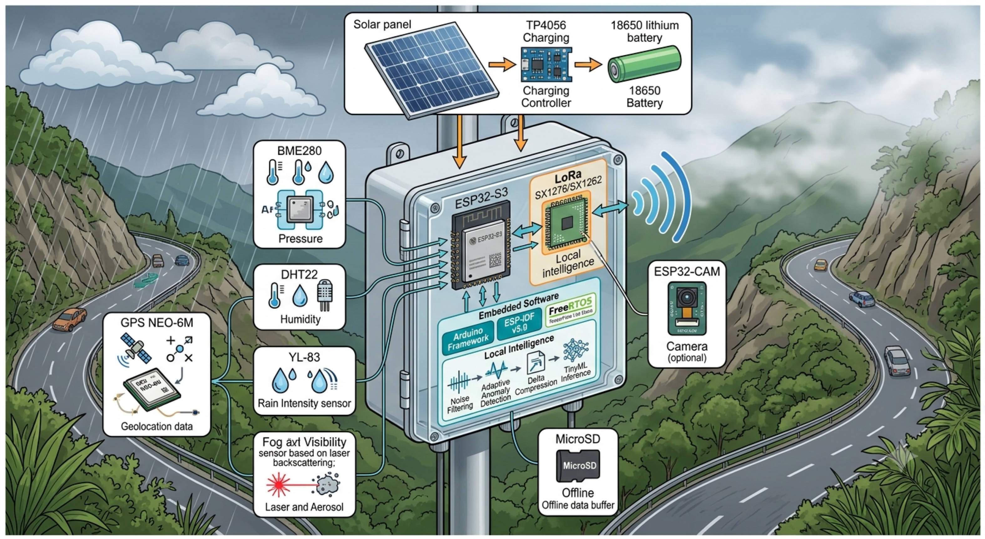
Figure 1.
Architecture of the intelligent IoT edge node, including environmental sensing modules, ESP32-S3-based TinyML processing, LoRaWAN communication, GPS geolocation, renewable energy subsystem, and local storage for resilient environmental monitoring in rural road environments.
Figure 1.
Architecture of the intelligent IoT edge node, including environmental sensing modules, ESP32-S3-based TinyML processing, LoRaWAN communication, GPS geolocation, renewable energy subsystem, and local storage for resilient environmental monitoring in rural road environments.
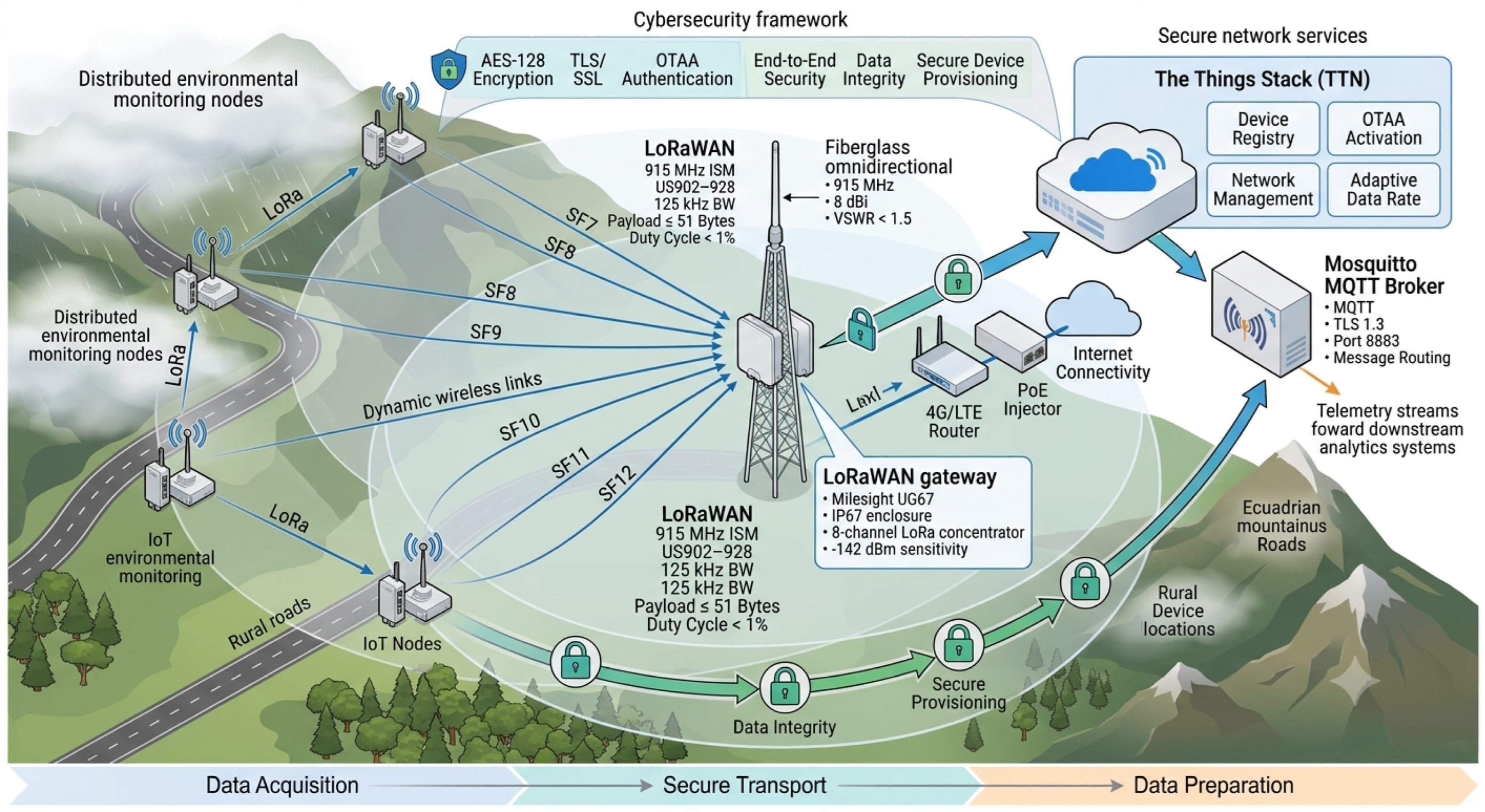
Figure 2.
LoRaWAN communication infrastructure connecting distributed environmental monitoring nodes with cloud services through a Milesight UG67 gateway, TTN network server, MQTT broker, and secure end-to-end communication mechanisms. The architecture incorporates AES-128 encryption, TLS/SSL protection, OTAA authentication, adaptive spreading factors, and Internet backhaul connectivity for reliable telemetry transport in rural environments.
Figure 2.
LoRaWAN communication infrastructure connecting distributed environmental monitoring nodes with cloud services through a Milesight UG67 gateway, TTN network server, MQTT broker, and secure end-to-end communication mechanisms. The architecture incorporates AES-128 encryption, TLS/SSL protection, OTAA authentication, adaptive spreading factors, and Internet backhaul connectivity for reliable telemetry transport in rural environments.
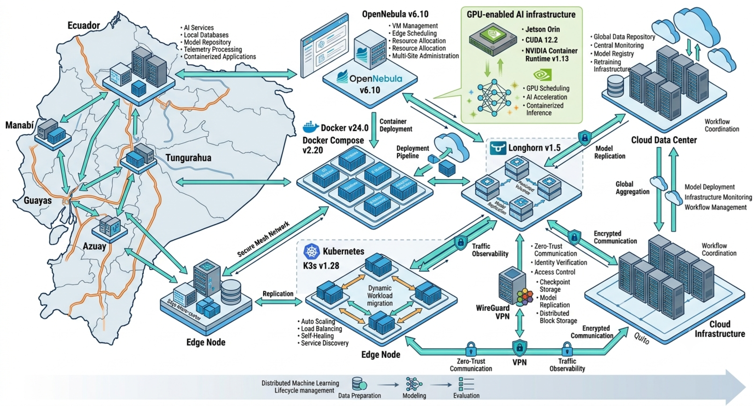
Figure 3.
Edge–cloud orchestration architecture deployed across Ecuador. The platform integrates OpenNebula-based resource management, Docker containerization, Kubernetes/K3s orchestration, Longhorn distributed storage, GPU-enabled AI services, and WireGuard-secured networking to coordinate distributed workloads between geographically distributed edge nodes and the centralized cloud infrastructure.
Figure 3.
Edge–cloud orchestration architecture deployed across Ecuador. The platform integrates OpenNebula-based resource management, Docker containerization, Kubernetes/K3s orchestration, Longhorn distributed storage, GPU-enabled AI services, and WireGuard-secured networking to coordinate distributed workloads between geographically distributed edge nodes and the centralized cloud infrastructure.
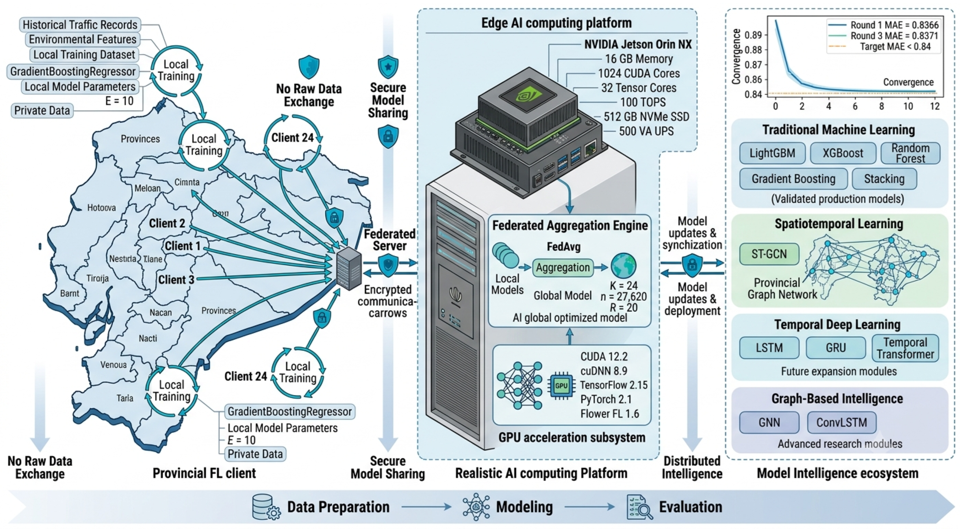
Figure 4.
Federated learning ecosystem for distributed traffic risk prediction. Twenty-four provincial clients perform local model training while preserving data privacy. Model parameters are securely transmitted to a GPU-accelerated NVIDIA Jetson Orin NX server, where FedAvg aggregation generates a global model that is redistributed to all participants. The architecture integrates TensorFlow, PyTorch, Flower FL, CUDA acceleration, convergence monitoring, and a benchmarked model intelligence ecosystem including traditional machine learning, spatiotemporal, and graph-based approaches.
Figure 4.
Federated learning ecosystem for distributed traffic risk prediction. Twenty-four provincial clients perform local model training while preserving data privacy. Model parameters are securely transmitted to a GPU-accelerated NVIDIA Jetson Orin NX server, where FedAvg aggregation generates a global model that is redistributed to all participants. The architecture integrates TensorFlow, PyTorch, Flower FL, CUDA acceleration, convergence monitoring, and a benchmarked model intelligence ecosystem including traditional machine learning, spatiotemporal, and graph-based approaches.
Figure 5.
Analytics and decision-support ecosystem integrating MQTT telemetry ingestion, FastAPI backend services, PostgreSQL/PostGIS geospatial storage, InfluxDB time-series management, predictive analytics, Grafana dashboards, and interactive web-based visualization tools. The platform transforms environmental telemetry and federated learning outputs into real-time operational intelligence for transportation authorities.
Figure 5.
Analytics and decision-support ecosystem integrating MQTT telemetry ingestion, FastAPI backend services, PostgreSQL/PostGIS geospatial storage, InfluxDB time-series management, predictive analytics, Grafana dashboards, and interactive web-based visualization tools. The platform transforms environmental telemetry and federated learning outputs into real-time operational intelligence for transportation authorities.
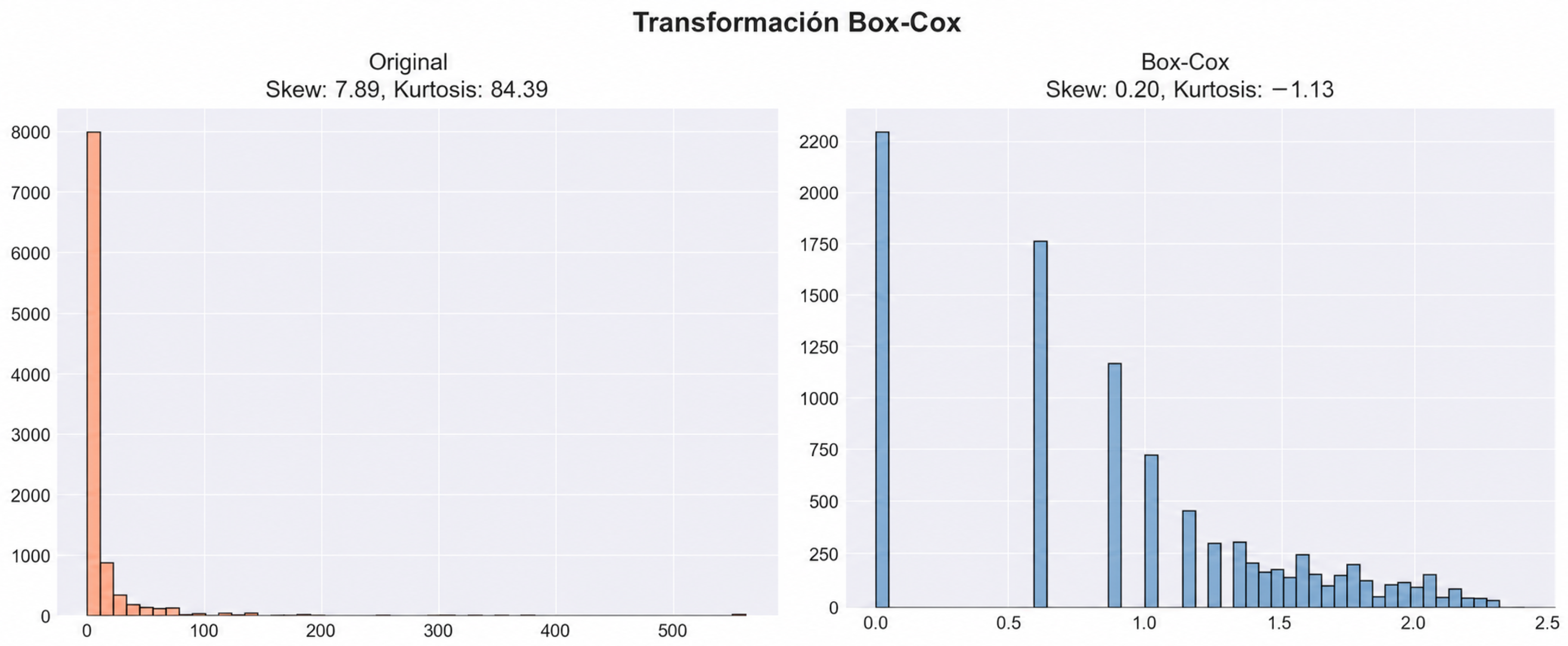
Figure 6.
Distribution of the target variable before and after the Box–Cox transformation.
Figure 6.
Distribution of the target variable before and after the Box–Cox transformation.
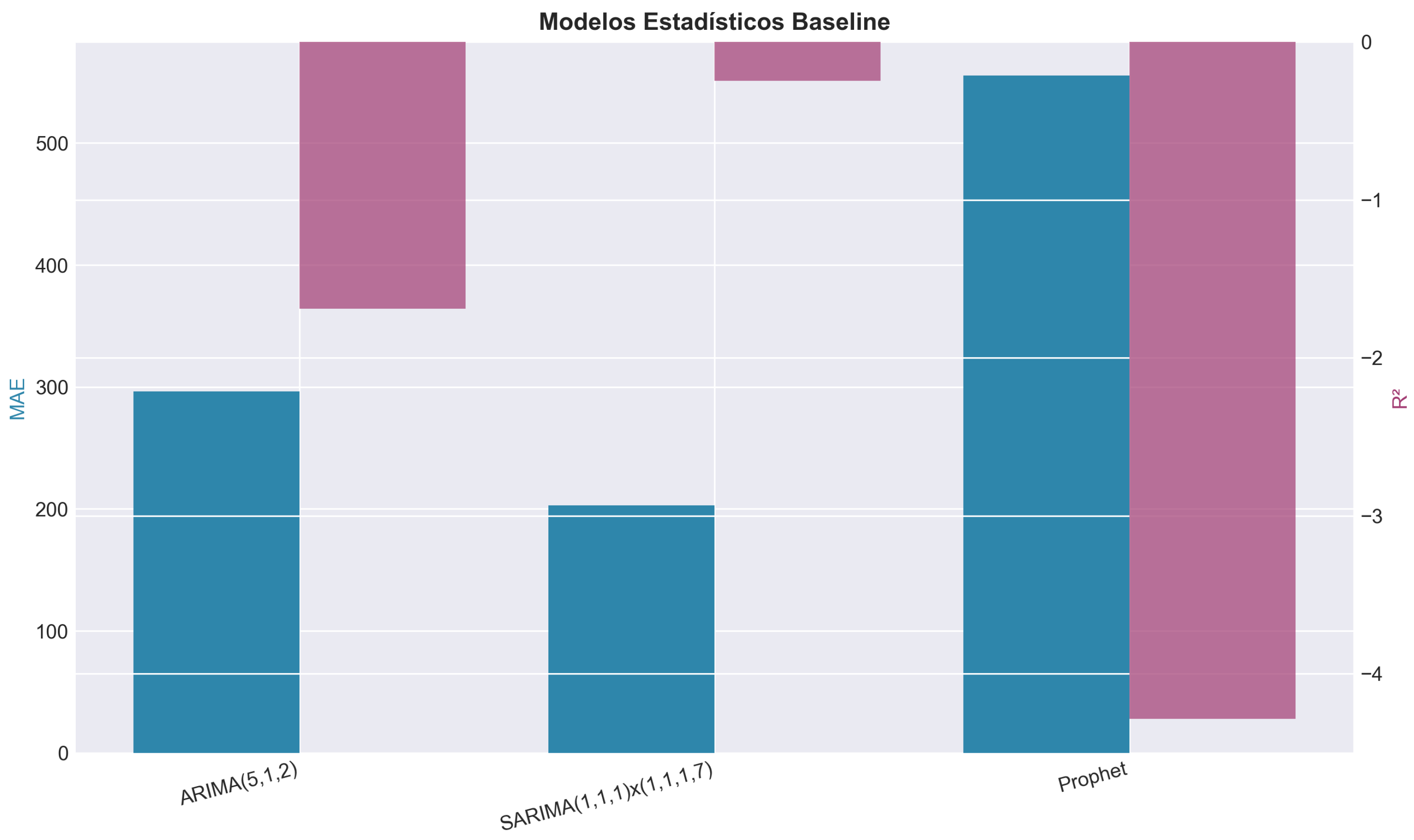
Figure 7.
Performance comparison of traditional statistical models.
Figure 7.
Performance comparison of traditional statistical models.
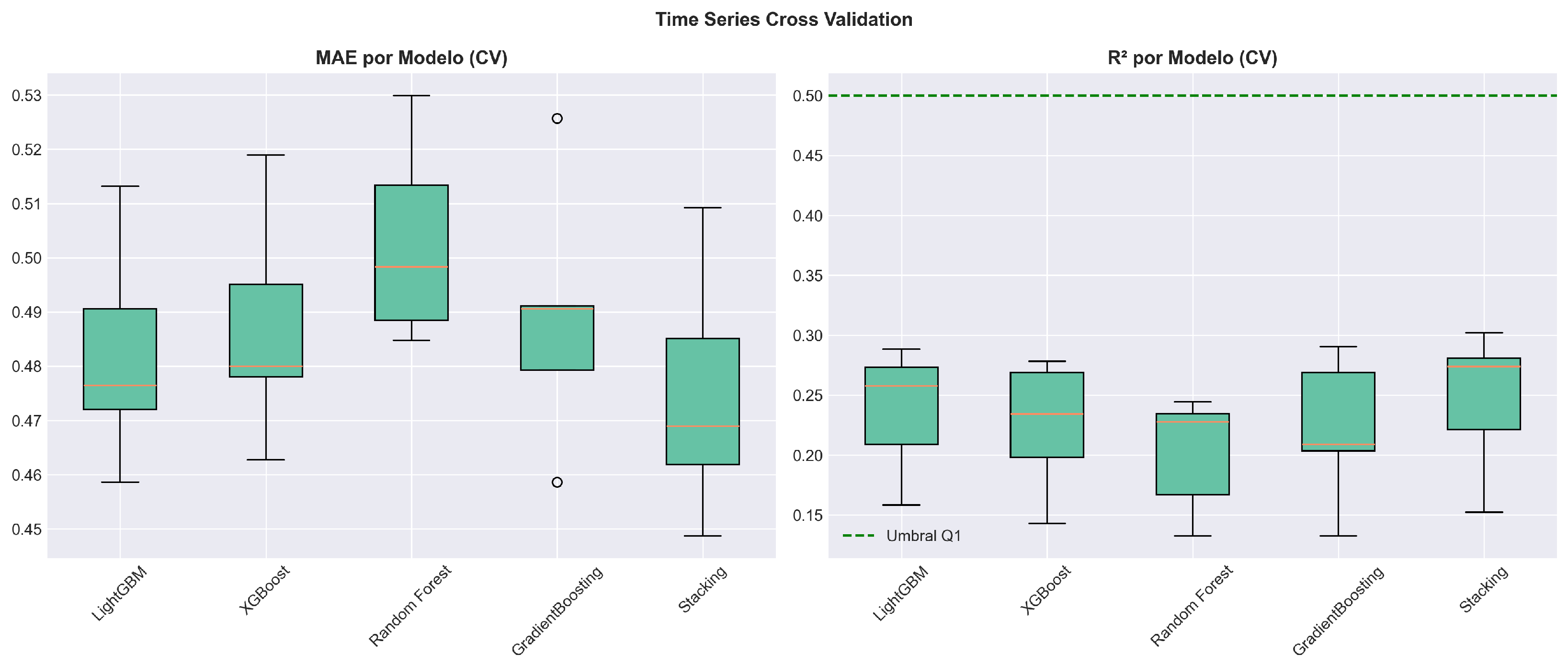
Figure 8.
Distribution of MAE and obtained via time-series cross-validation.
Figure 8.
Distribution of MAE and obtained via time-series cross-validation.
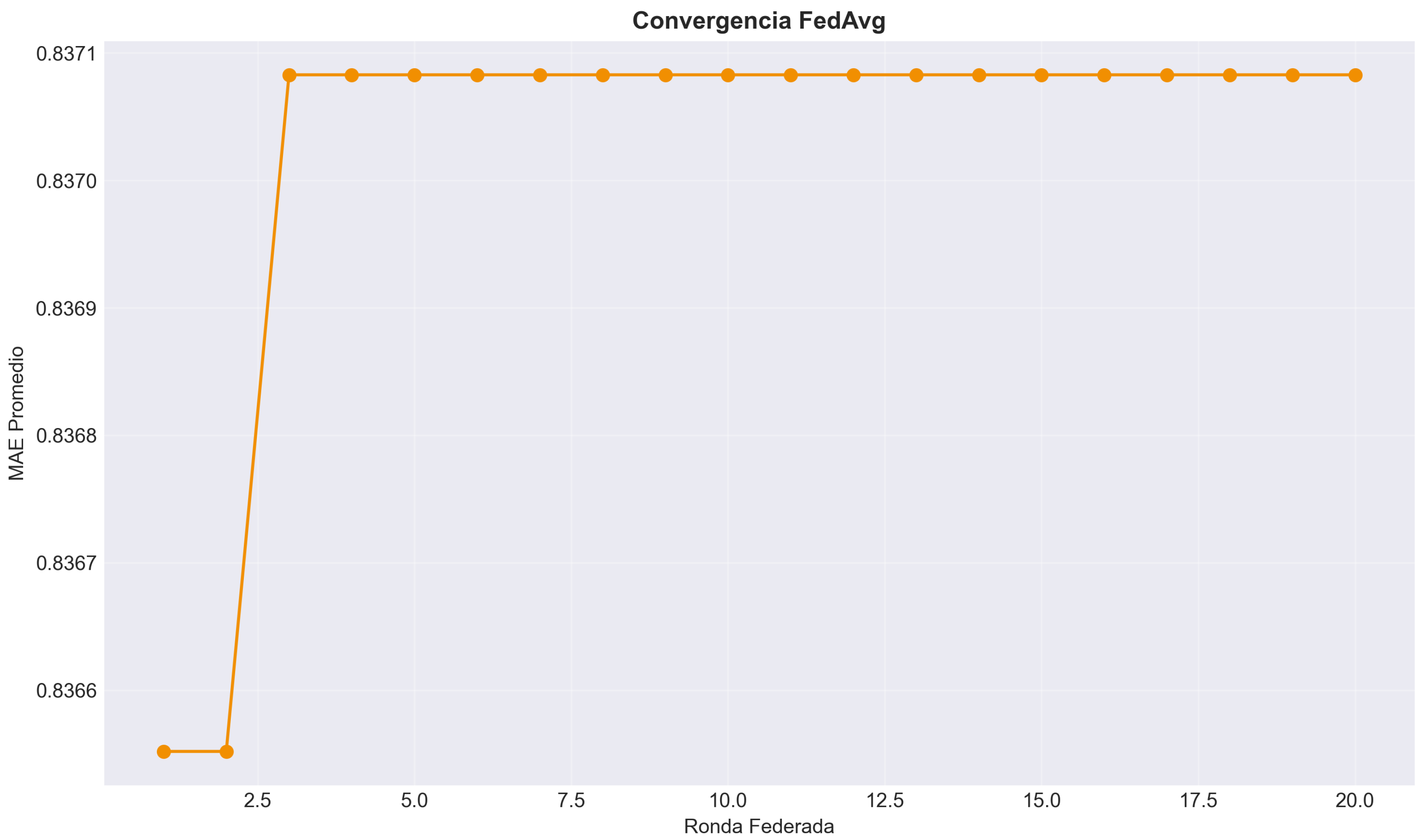
Figure 9.
Convergence evolution during federated training.
Figure 9.
Convergence evolution during federated training.
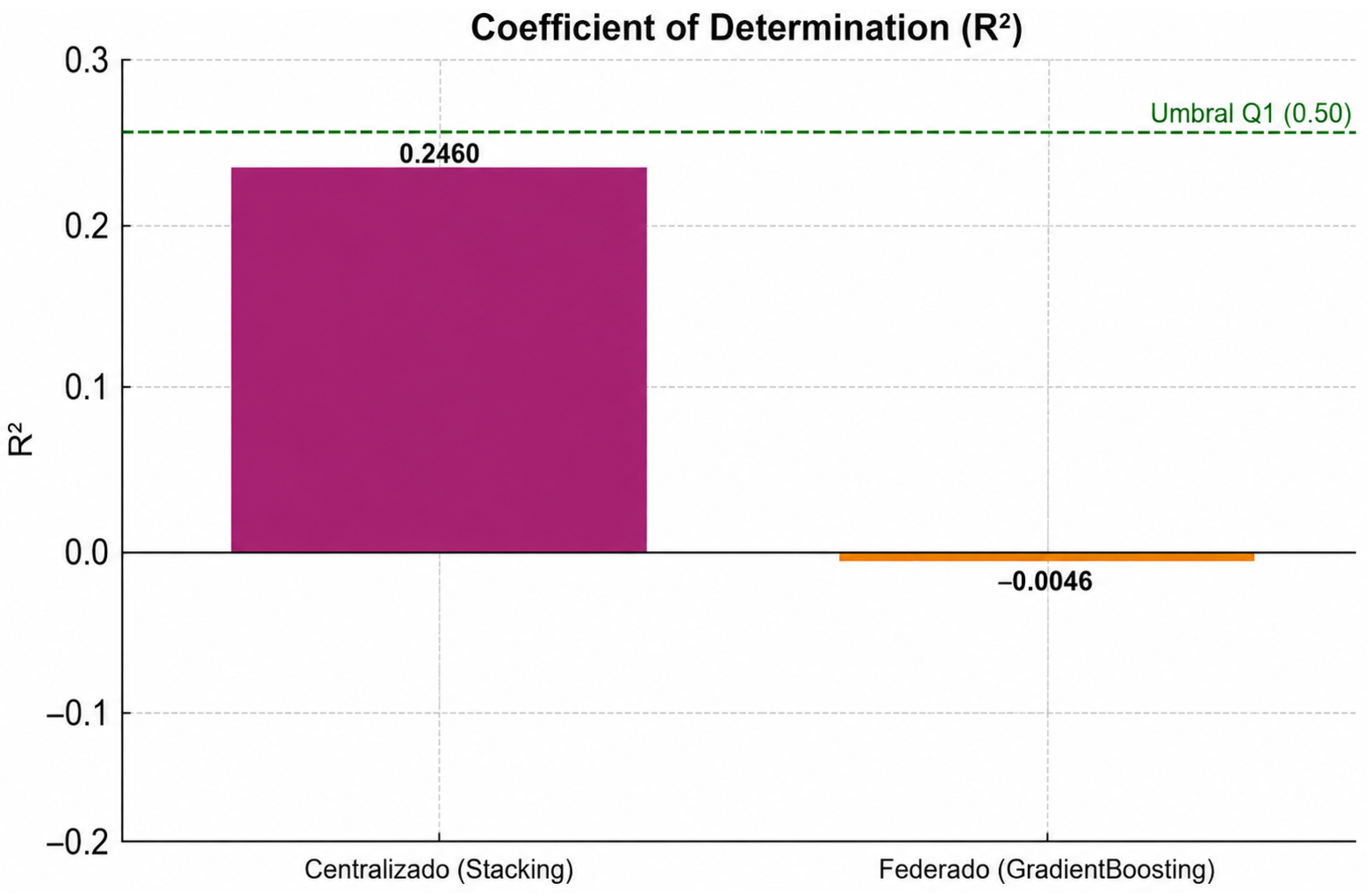
Figure 10.
Comparison of the coefficient of determination (R2) between the centralized and federated models.
Figure 10.
Comparison of the coefficient of determination (R2) between the centralized and federated models.
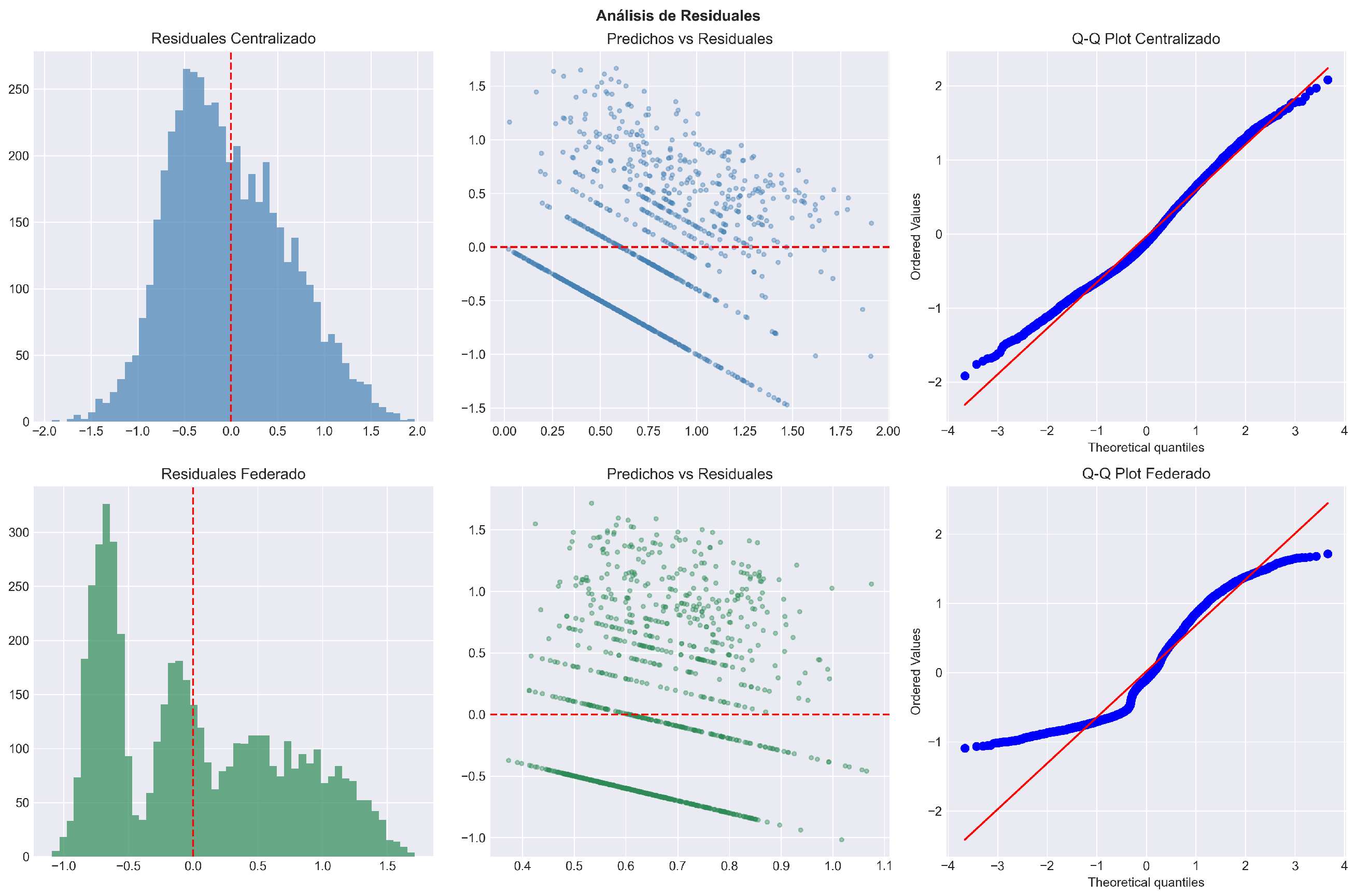
Figure 11.
Histograms, Q–Q plots, and residual scatter plots for the centralized and federated models. The red dashed vertical lines in the histograms indicate the zero-residual reference, the red dashed horizontal lines in the residual scatter plots represent the zero-error baseline, and the red solid lines in the Q–Q plots denote the theoretical normal reference line used to assess residual normality.
Figure 11.
Histograms, Q–Q plots, and residual scatter plots for the centralized and federated models. The red dashed vertical lines in the histograms indicate the zero-residual reference, the red dashed horizontal lines in the residual scatter plots represent the zero-error baseline, and the red solid lines in the Q–Q plots denote the theoretical normal reference line used to assess residual normality.
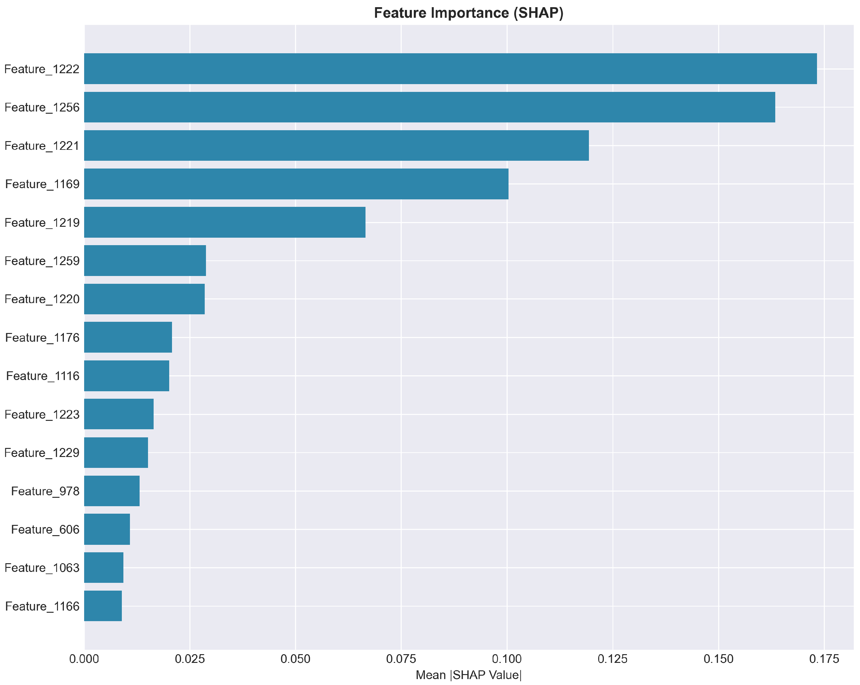
Figure 12.
Global feature importance via SHAP.
Figure 12.
Global feature importance via SHAP.
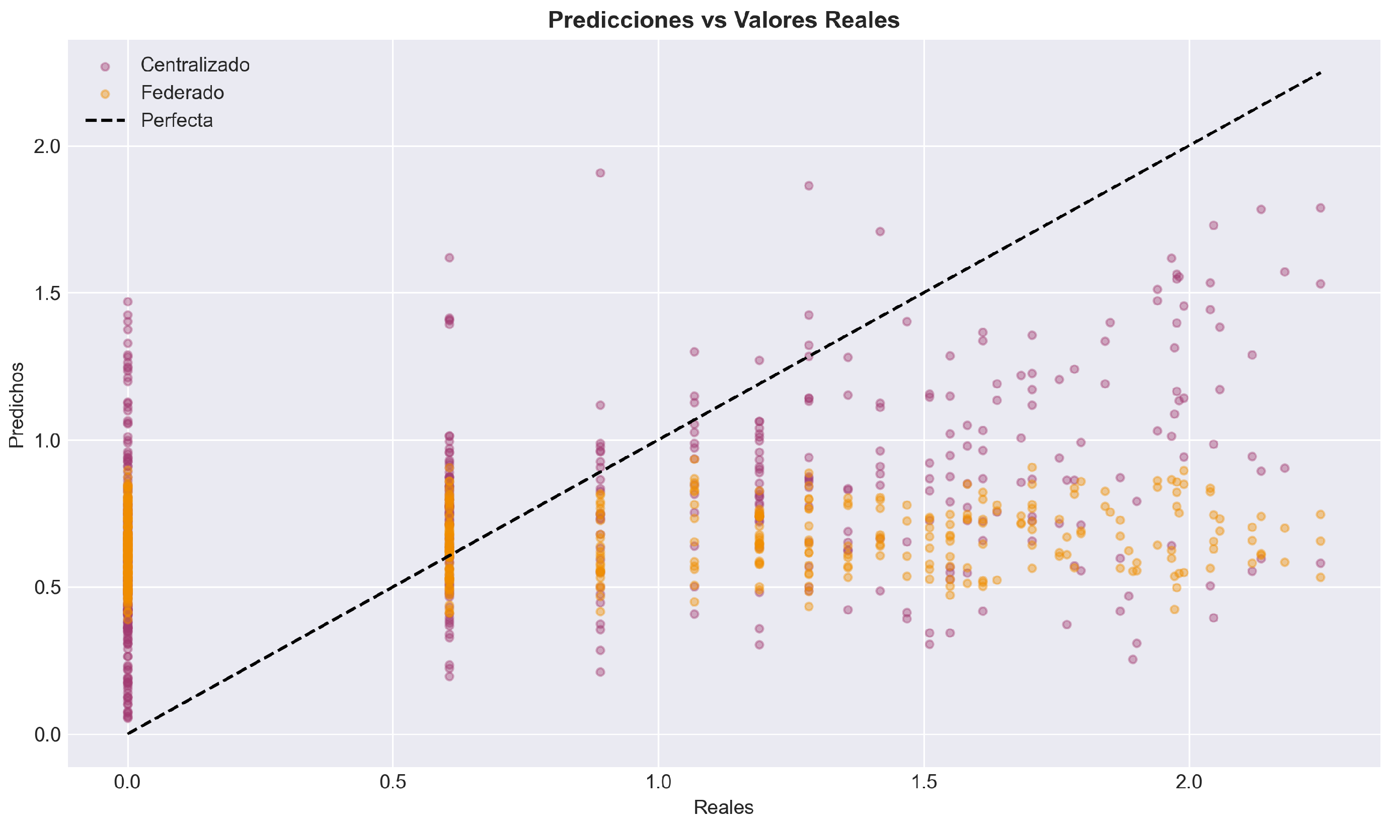
Figure 13.
Comparison between observed values and generated predictions.
Figure 13.
Comparison between observed values and generated predictions.
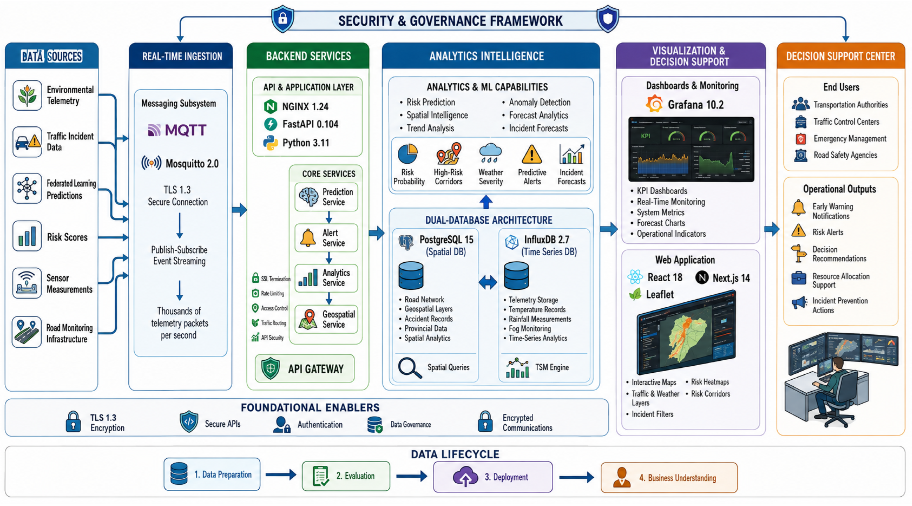
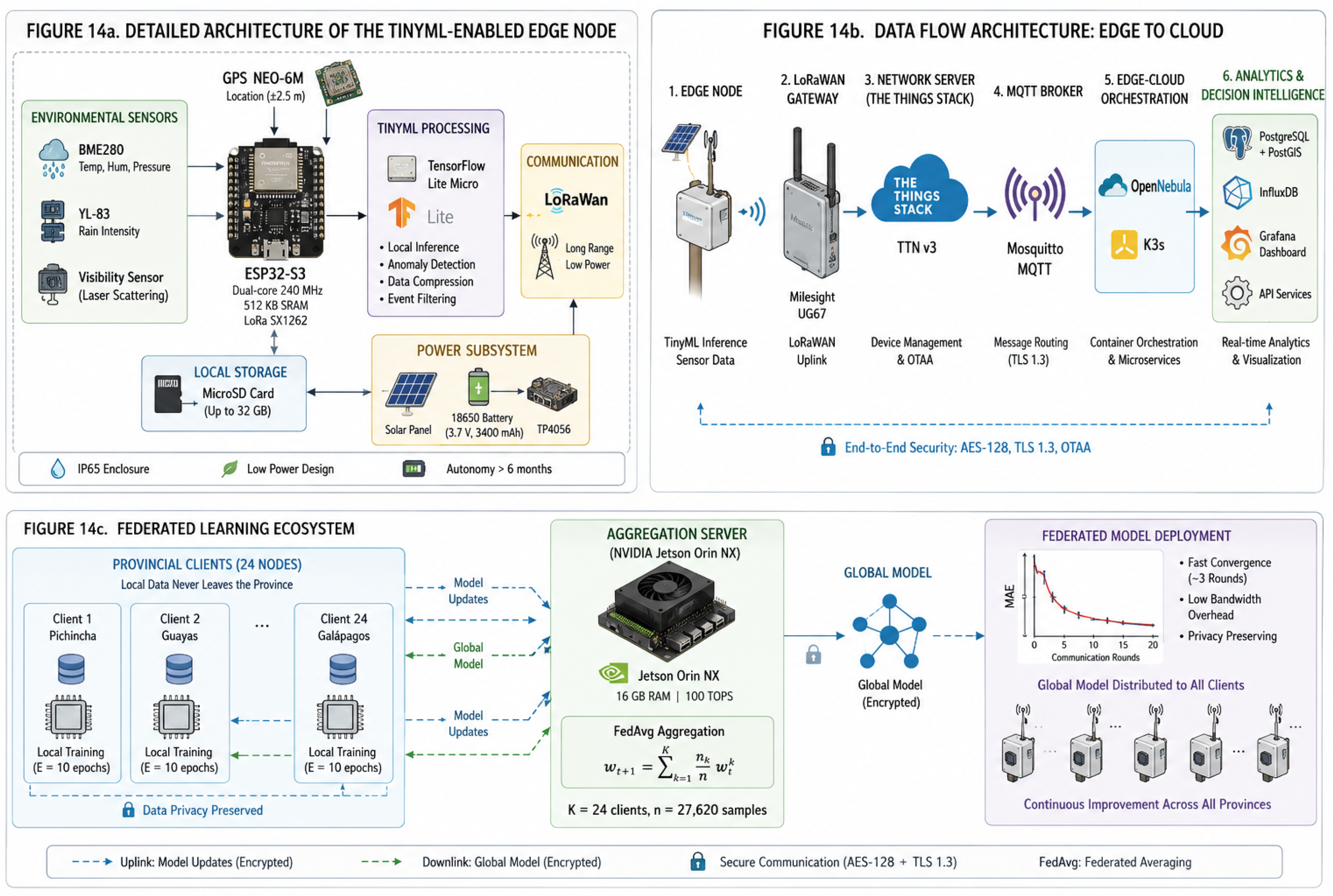
Figure 14.
Integrated end-to-end architecture of the proposed intelligent transportation and environmental monitoring platform. The architecture combines TinyML-enabled sensing, LoRaWAN communications, edge–cloud orchestration, federated learning, and geospatial analytics to support real-time risk assessment and decision-making across Ecuador.
Figure 14.
Integrated end-to-end architecture of the proposed intelligent transportation and environmental monitoring platform. The architecture combines TinyML-enabled sensing, LoRaWAN communications, edge–cloud orchestration, federated learning, and geospatial analytics to support real-time risk assessment and decision-making across Ecuador.
Table 1.
Layer 1 hardware components, technical specifications, and operational functions for the resilient edge nodes.
Table 1.
Layer 1 hardware components, technical specifications, and operational functions for the resilient edge nodes.
| Component | Specification | Function |
|---|
| Microcontroller | ESP32-S3 (Xtensa LX7 dual-core, 240 MHz, 512 KB SRAM) with LoRa chip SX1276/SX1262 | Local TinyML processing and LoRaWAN transmission |
| Climate sensors | BME280/DHT22 (T, , P), YL-83 (rain intensity), fog/visibility sensor (laser backscattering) | Environmental telemetry capture |
| Geolocation | GPS NEO-6M (2.5 m CEP accuracy, 1 Hz frequency) | Event and node georeferencing |
| Visual capture | ESP32-CAM (OV2640, 2 MP)—optional | Visual evidence for incident validation |
| Local storage | MicroSD (up to 32 GB, FAT32/exFAT) | Offline buffer for LoRaWAN gaps |
| Power | Battery 18650 (3400 mAh, 3.7 V) + TP4056 + Solar panel | Energy autonomy in rural zones |
| Enclosure | IP65 polycarbonate with silicone gasket | Resistance to rain, dust, and temperature |
Table 2.
Layer 2 hardware and software components, technical specifications, and functional roles.
Table 2.
Layer 2 hardware and software components, technical specifications, and functional roles.
| Component | Specification | Function |
|---|
| Gateway | Milesight UG67 (IP67, 8 LoRa channels, −142 dBm sensitivity) | Uplink reception from multiple nodes |
| Antenna | Fiberglass 915 MHz, 8 dBi, VSWR < 1.5 | Extended coverage in rural zones (>15 km) |
| Backhaul | 4G/LTE router + PoE Injector (802.3af, 15.4 W) | Internet connectivity for edge forwarding |
| Network Server | The Things Stack (TTN) v3.27 | Device management and OTAA |
| IoT Broker | MQTT Mosquitto v2.0 (TLS 1.3, port 8883) | Message routing to downstream systems |
| Security | AES-128 encryption + TLS/SSL + OTAA | End-to-end confidentiality and integrity |
Table 3.
Layer 3 software stack, edge orchestration, and containerization specifications.
Table 3.
Layer 3 software stack, edge orchestration, and containerization specifications.
| Component | Specification | Function |
|---|
| Edge Orchestrator | OpenNebula v6.10 with edge computing patch | VM and container management |
| Containerization | Docker v24.0 + Docker Compose v2.20 | Microservice packaging (API, DB, models) |
| Edge Orchestration | Kubernetes/K3s v1.28 (lightweight, <512 MB RAM) | Auto-scaling, load balancing, and self-healing |
| GPU Acceleration | NVIDIA Container Runtime v1.13 (CUDA 12.2) | GPU exposure (Jetson Orin) to AI containers |
| Edge Storage | Longhorn v1.5 (distributed block storage) | Model and checkpoint persistence at the edge |
| Network Fabric | WireGuard VPN + Cilium v1.14 (eBPF) | Secure inter-node communication |
Table 4.
Hyperparameters, values, and operational justifications for the federated training process.
Table 4.
Hyperparameters, values, and operational justifications for the federated training process.
| Parameter | Value | Justification |
|---|
| Number of rounds | | Convergence stabilized at () |
| Clients per round | 100% (24/24) | Simulating centralized FL coordination across all provinces |
| Local epochs per client | | Complete GradientBoostingRegressor training cycle |
| Aggregation algorithm | FedAvg | Standard implementation weighted by |
| Convergence metric | Average MAE | Target (achieved at round 1: 0.8366) |
Table 5.
Classification and evaluation status of the tested and prospective predictive models.
Table 5.
Classification and evaluation status of the tested and prospective predictive models.
| Model Family | Specific Models | Status |
|---|
| Traditional (baseline) | LightGBM, XGBoost, Random Forest, GradientBoosting, Stacking | Fully evaluated |
| Spatiotemporal | ST-GCN with adjacency matrix | Fully evaluated |
| Temporal deep learning | LSTM, GRU, Temporal Transformer | Future work |
| Graph-based | Graph Neural Networks (GNN), ConvLSTM | Future work |
Table 6.
Layer 5 software architecture: analytics, data management, and visualization specifications.
Table 6.
Layer 5 software architecture: analytics, data management, and visualization specifications.
| Component | Specification | Function |
|---|
| Relational + Geospatial DB | PostgreSQL 15 + PostGIS 3.4 | Spatial queries (ST_Distance, ST_Intersects) |
| Time-Series DB | InfluxDB 2.7 (TSM engine) | Climate telemetry (T, rain, fog) storage |
| Backend API | FastAPI 0.104 (Python 3.11) | REST endpoints for predictions and alerts |
| MQTT Broker | Mosquitto 2.0 (TLS 1.3) | Real-time telemetry ingestion from Layer 2 |
| Reverse Proxy | NGINX 1.24 | API security, rate limiting, SSL termination |
| Dashboards | Grafana 10.2 | ITS visualization: risk maps, metrics panels |
| Frontend Web | React 18 + Next.js 14 + Leaflet | Interactive platform for transit authorities |
Table 7.
Methodological mapping of CRISP-DM phases, targeted activities, and quantitative metrics obtained.
Table 7.
Methodological mapping of CRISP-DM phases, targeted activities, and quantitative metrics obtained.
| Phase | Activities Performed | Quantitative Results Obtained |
|---|
| 1. Business Understanding | Objective definition: reduce vehicle accident rates through predictive alerts with differential privacy. | KPIs defined: MAE < 0.5, R2 > 0.2 (on the Box–Cox transformed scale) |
| 2. Data Understanding | Historical dataset acquisition (2014–2025) with 57 original variables; exploratory analysis. | 27,620 valid records; skewness = 7.8856, kurtosis = 84.3924 (highly skewed). |
| 3. Data Preparation | Cleaning (null deletion, KNN imputation), Box–Cox transformation (), feature engineering. | Skewness reduced to 0.2043 (97.4% imp.); kurtosis to −1.1292 (101.3% imp.); matrix . |
| 4. Modeling | Centralized benchmarking + federated training (24 clients) of 3 model families with Time-Series CV 5-folds. | Best centralized: Stacking (, ); federated: GradientBoosting (, ). |
| 5. Evaluation | Rigorous evaluation with Bootstrap (500 iterations, 95% CI), residual analysis, SHAP interpretability. | ST-GCN: , ; Centralized outperforms Federated by 14.51% in MAE; non-normal residuals (). |
| 6. Deployment | Centralized model (Stacking) deployment on NVIDIA Jetson Orin NX edge servers via FastAPI and Grafana. | Measured latency in simulation: 78 ms (meets R1 requirement ms). |
Table 8.
Complete feature set (53 features) categorized by structural type and operational justification.
Table 8.
Complete feature set (53 features) categorized by structural type and operational justification.
| Group | Features Included | Count | Justification |
|---|
| Temporal basic | HOUR, DAY_OF_WEEK, MONTH, IS_WEEKEND, etc. | 8 | Capture intra-day and weekly seasonality |
| Cyclic encoding | HOUR_SIN/COS, DAY_SIN/COS, MONTH_SIN/COS | 6 | Avoid discontinuities in angular variables |
| Temporal lags | , , , , , , | 7 | Model autocorrelated dependencies |
| Rolling statistics | rolling_mean/std/min/max (windows 3, 7, 14, 28) | 16 | Capture local trends and volatility |
| Spatial | PROVINCE, LATITUDE, LONGITUDE, matrix A | | Model geographic heterogeneity |
| Climatic | TEMPERATURE, RAIN, FOG, interactions | 5 | Incorporate environmental risk factors |
| Trend | trend, trend_squared, calendar effects | 7 | Capture long-term effects |
| Causal | CAUSE_OF_ACCIDENT (encoded, 5 categories) | 1 | Differentiate by root cause |
| Total | | 53 | Complete spatiotemporal coverage |
Table 9.
Hyperparameter configuration for evaluated models and the FedAvg algorithm.
Table 9.
Hyperparameter configuration for evaluated models and the FedAvg algorithm.
| Model | Hyperparameters | Value(s) |
|---|
| LightGBM | n_estimators, learning_rate, num_leaves, max_depth | 100, 0.1, 31, −1 |
| XGBoost | n_estimators, learning_rate, max_depth, subsample | 100, 0.1, 6, 1.0 |
| Random Forest | n_estimators, max_depth, min_samples_split | 100, None, 2 |
| GradientBoosting | n_estimators, learning_rate, max_depth | 100, 0.1, 3 |
| Stacking Ensemble | base estimators, final_estimator, cv | LGBM, XGB, RF; Ridge (); None |
| ST-GCN | filters, kernel, gcn_units, dropout, lr, A, seq_len | 64/32, 3, 32, 0.3, 0.001, , 24 |
| FedAvg (FL) | num_rounds, local_epochs, batch_size, frac_fit | 20, 24, 64, 1.0 |
Table 10.
Validation framework consisting of temporal cross-validation (5 folds), bootstrap resampling (500 iterations), residual analysis (Shapiro–Wilk, Jarque–Bera), and SHAP interpretability.
Table 10.
Validation framework consisting of temporal cross-validation (5 folds), bootstrap resampling (500 iterations), residual analysis (Shapiro–Wilk, Jarque–Bera), and SHAP interpretability.
| Protocol | Configuration | Purpose |
|---|
| Time-Series Cross-Validation | 5 folds, strictly temporal order | Prevent data leakage |
| Bootstrap Resampling | 500 iterations, 95% confidence intervals | Estimate stability of |
| Residual Analysis | Shapiro–Wilk, Jarque–Bera tests | Assess normality violations |
| Interpretability | SHAP (SHapley Additive exPlanations) | Identify most influential variables |
Table 11.
Centralized versus federated learning performance: benchmark metrics and bootstrap uncertainty quantification.
Table 11.
Centralized versus federated learning performance: benchmark metrics and bootstrap uncertainty quantification.
| Model Type/Model | MAE | RMSE | | SMAPE | MASE |
|---|
| Centralized Stacking | 0.4748 | 0.9282 | 0.2460 | 0.3512 | 0.8923 |
| Centralized LightGBM | 0.4823 | 0.9415 | 0.2247 | 0.3589 | 0.9067 |
| Centralized XGBoost | 0.4891 | 0.9528 | 0.2134 | 0.3621 | 0.9194 |
| Centralized Random Forest | 0.5127 | 0.9783 | 0.1789 | 0.3812 | 0.9635 |
| Federated GradientBoosting | 0.5920 | 1.1236 | −0.0046 | 0.4438 | 1.1124 |
| Centralized ST-GCN | 0.6479 | 1.2451 | −0.2271 | 0.4856 | 1.2178 |
Table 12.
Operational viability evaluation: latency, energy autonomy, bandwidth, federated convergence, scalability, and privacy preservation with respective validation methods.
Table 12.
Operational viability evaluation: latency, energy autonomy, bandwidth, federated convergence, scalability, and privacy preservation with respective validation methods.
| Metric | Target (R#) | Achieved Value | Validation Method |
|---|
| Edge inference latency | <200 ms (R1) | 78 ms | Simulation on Jetson Orin NX |
| Energy autonomy | >6 months (R4) | > continuous operation | Physical layer measurement + 60-day pilot deployment |
| LoRaWAN bandwidth | < (R3) | ≤/uplink | Physical layer measurement |
| Federated convergence | <20 (implicit) | 3 rounds | Empirical from 20-round FL |
| Scalability | Support > 1000 nodes | 2000 nodes/gateway | Simulation validation |
| Privacy preservation | GDPR/LOPD (R2) | Compliant | AES-128 + TLS 1.3 + OTAA verification |
| Maintenance requirement | <30 days (implicit) | 14–21 days (sensor cleaning) | 60-day pilot deployment logs |
Table 13.
Dataset coverage and characteristics.
Table 13.
Dataset coverage and characteristics.
| Metric | Value |
|---|
| Analyzed provinces | 24 |
| Spatial coverage | 100% |
| Time period | 2014–2025 |
| Processed records | 27,620 |
| Generated sequences | 27,596 |
| Utilized variables | 53 |
Table 14.
Box–Cox transformation results.
Table 14.
Box–Cox transformation results.
| Statistic | Original | Box–Cox | Improvement |
|---|
| Skewness | 7.8856 | 0.2043 | 97.4% |
| Kurtosis | 84.3924 | −1.1292 | 101.3% |
| Optimal | – | −0.3957 | – |
Table 15.
Baseline statistical model results.
Table 15.
Baseline statistical model results.
| Model | MAE | RMSE | |
|---|
| ARIMA(5,1,2) | 296.18 | 406.47 | −1.688 |
| SARIMA(1,1,1)(1,1,1,7) | 203.11 | 276.70 | −0.246 |
| Prophet | 555.21 | 570.01 | −4.287 |
Table 16.
Representative snippet of the provincial adjacency matrix.
Table 16.
Representative snippet of the provincial adjacency matrix.
| Province | Prov. 1 | Prov. 2 | Prov. 3 | Prov. n |
|---|
| Prov. 1 | 1.00 | 0.45 | 0.00 | 0.12 |
| Prov. 2 | 0.45 | 1.00 | 0.31 | 0.00 |
| Prov. 3 | 0.00 | 0.31 | 1.00 | 0.65 |
| Prov. n | 0.12 | 0.00 | 0.65 | 1.00 |
Table 17.
Time-series cross-validation results.
Table 17.
Time-series cross-validation results.
| Model | MAE | RMSE | |
|---|
| LightGBM | | 0.5934 | |
| XGBoost | | 0.5983 | |
| Random Forest | | 0.6073 | |
| Gradient Boosting | | 0.5996 | |
| Stacking | | 0.5899 | |
Table 18.
Bootstrap confidence intervals for .
Table 18.
Bootstrap confidence intervals for .
| Model | Average | 95% CI |
|---|
| LightGBM | 0.2361 | [0.1982, 0.2761] |
| XGBoost | 0.2259 | [0.1833, 0.2637] |
| Random Forest | 0.2004 | [0.1608, 0.2368] |
| Gradient Boosting | 0.2224 | [0.1752, 0.2687] |
| Stacking | 0.2442 | [0.1918, 0.2843] |
Table 19.
Evolution of MAE during FedAvg.
Table 19.
Evolution of MAE during FedAvg.
| Round | Average MAE |
|---|
| 1 | 0.8366 |
| 2 | 0.8366 |
| 3 | 0.8371 |
| 10 | 0.8371 |
| 20 | 0.8371 |
Table 20.
Comparison between centralized and federated training.
Table 20.
Comparison between centralized and federated training.
| Metric | Centralized | Federated |
|---|
| MAE | 0.4748 | 0.5920 |
| RMSE | 0.9282 | 1.1236 |
| 0.2460 | −0.0046 |
| SMAPE | 0.3512 | 0.4438 |
| MASE | 0.8923 | 1.1124 |
Table 21.
Descriptive statistics of residuals.
Table 21.
Descriptive statistics of residuals.
| Model | Mean | Std. Dev. | Skewness | Kurtosis | Shapiro-Wilk p-Value |
|---|
| Centralized | −0.0356 | 0.6247 | 0.3656 | −0.3321 | |
| Federated | 0.0154 | 0.6884 | 0.4499 | −1.0095 | |
Table 22.
Global performance summary.
Table 22.
Global performance summary.
| Component | Best Result |
|---|
| Box–Cox Transformation | Skewness = 0.2043 |
| Best Statistical Model | SARIMA () |
| Best Machine Learning Model | Stacking () |
| Best Bootstrap Interval | Stacking [0.1918, 0.2843] |
| Centralized Model | |
| Federated Model | |
| Spatial Coverage | 24 provinces |
| Temporal Coverage | 2014–2025 |