Adjoint-Based Joint Reconstruction of Heat Source and Initial Condition with Uncertainty Quantification

Abstract

This paper develops an adjoint-based framework for jointly reconstructing a space–time-dependent internal heat source and an unknown initial temperature field from sparse, noisy measurements. A single adjoint solve supplies the gradients with respect to both fields, so each iteration requires one forward and one adjoint solve. Deterministically, CGLS with discrepancy-principle stopping reaches a comparable regularized solution in about an order of magnitude fewer iterations than Landweber–Fridman. In the Bayesian formulation, Gaussian noise and Matérn priors yield an exact Gaussian posterior; prior-preconditioned conjugate gradients compute the maximum a posteriori estimate, while a low-rank approximation of the prior-preconditioned data-misfit Hessian provides pointwise credible bands. The exact discrete adjoint gives machine-precision gradients, and prior-predictive experiments verify nominal pointwise coverage. Numerical experiments compare the reconstructions and assess sensitivity to noise, discretization, and prior hyperparameters. The Bayesian reconstruction is more accurate and mesh-robust in the reported tests. A calibrated generalized-${\chi }^2$ discrepancy diagnostic detects misspecification caused by an omitted initial-temperature offset and, less strongly, by discontinuous sources outside the prior model. These experiments demonstrate joint reconstruction and scalable uncertainty quantification using only forward and adjoint heat-equation solves.

1. Introduction

Internal heat generation in a conducting body is usually not measurable directly. What can be measured is temperature at a small number of locations and over a finite time window, and the source must then be inferred by inverting the heat equation. This inverse source problem has a long history, both in the heat transfer literature [1,2,3] and in the theory of inverse problems for parabolic equations [4,5,6]. A complication that arises in practice is that the initial temperature field is rarely known: experiments often begin before the specimen reaches equilibrium, or the initial state is instrumented only at the sensor locations. The unknown initial condition must therefore be estimated together with the source, since errors in the assumed initial state propagate into the source estimate.

Both unknowns enter the parabolic problem linearly; nevertheless, the joint reconstruction is severely ill-posed. Diffusion strongly attenuates high spatial frequencies—exponentially for initial-condition modes across a positive observation lag—and finitely many temperature measurements cannot uniquely identify an unrestricted space–time source [6,7]. Iterative regularization is a natural tool for problems of this type, attractive for problems constrained by partial differential equations (PDEs) because each step requires only one forward and one adjoint solve. Its classical instance is the Landweber–Fridman iteration [8,9], which applies the adjoint of the forward map to the data residual and takes a fixed-point step, with regularization supplied by stopping early, typically through Morozov’s discrepancy principle [10]. The convergence theory is well established [11,12,13]; the iteration is robust but slow, and Krylov subspace methods, namely conjugate-gradient least squares (CGLS) and its numerically stable implementation least-squares QR (LSQR) [14,15,16], reach the same regularized solution in far fewer adjoint solves and are the modern method of choice. Iterations of this kind have been used extensively for heat conduction problems, including the reconstruction of spacewise-dependent sources [17,18], source terms identified from final-time data [19,20], and Cauchy problems treated by the alternating method of Kozlov et al. [21]. Johansson and Lesnic [22] reconstructed a spacewise-dependent source, which is closest to the present setting, together with the initial temperature from two temperature snapshots, using a sequence of well-posed direct problems with discrepancy-principle stopping.

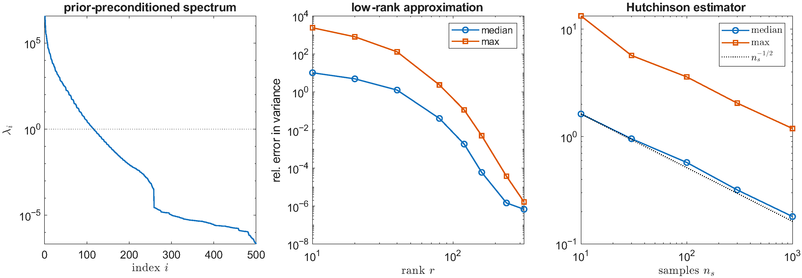
These deterministic schemes return a point estimate. They treat the noise only through the stopping rule and say nothing about the uncertainty that remains in the reconstruction, which matters whenever the estimate feeds a subsequent decision or design step. The statistical theory of inverse problems [23,24,25] supplies the missing layer: the unknowns are modeled as random fields, the noise enters through a likelihood, and the posterior distribution carries both the estimate and its uncertainty. For linear forward maps with Gaussian noise and Gaussian priors the posterior is Gaussian, and its covariance can be explored at scale through low-rank approximations of the data-misfit Hessian [26,27,28]. Bayesian formulations of thermal inverse problems, in particular, have been developed for parabolic equations with uncertain boundary data and for the calibration of wall thermal properties [29,30,31].

The contribution of this paper is an adjoint-based framework that treats the joint space–time source and initial-condition problem both deterministically and probabilistically and equips the reconstruction with calibrated uncertainty. Existing joint reconstructions are deterministic and restrict the source to a spacewise-dependent profile recovered from temperature snapshots [22]; here the source varies in both space and time, and the method returns point estimates together with calibrated pointwise credible bands for both unknown fields, at the cost of forward and adjoint solves of the heat equation. 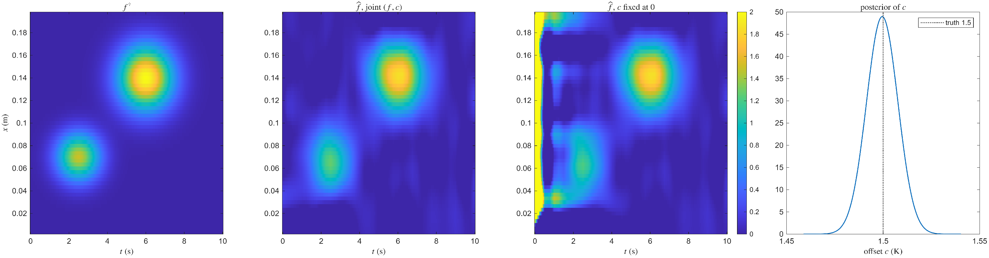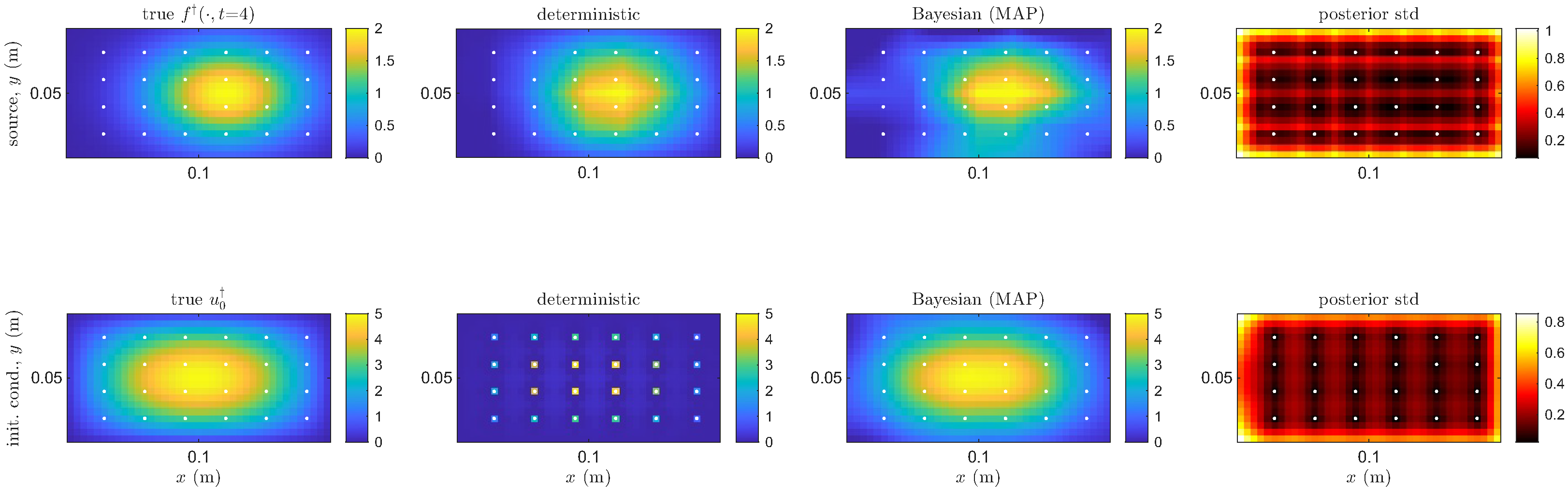The technical basis is an elementary fact that has not, to our knowledge, been exploited for this purpose: a single adjoint solve provides the gradient of the data misfit with respect to both unknowns, because the adjoint state in the interior is the gradient with respect to the source, while its trace at $t=0$ is the gradient with respect to the initial condition. On this joint gradient we build two reconstructions that share the same forward and adjoint machinery. The first is deterministic: the data misfit is minimized by conjugate-gradient least squares with statistical discrepancy-principle stopping, with the Landweber–Fridman iteration being retained as a baseline. The second is Bayesian: Gaussian priors render the posterior exactly Gaussian, its maximum a posteriori (MAP) estimate is computed by prior-preconditioned conjugate gradients, and the linearity of the forward map is exploited to obtain pointwise variances from a low-rank decomposition of the prior-preconditioned data-misfit Hessian. Because the discrete adjoint of the Crank–Nicolson scheme is implemented exactly, every gradient is correct to machine precision for the discrete objective, and the credible intervals are verified by a coverage experiment over truths drawn from the prior. We compare the deterministic and Bayesian reconstructions and study their robustness to the noise level and to the discretization; and a final example illustrates the practical value of the probabilistic viewpoint, in which a misspecified initial condition that a deterministic least-squares fit silently absorbs into the source is exposed by the calibrated discrepancy diagnostic. Although developed in one spatial dimension for clarity, the method is formulated for arbitrary dimension in Section 2 and demonstrated on a two-dimensional plate in Section 6.4; nothing in the construction is specific to one dimension.

The remainder of this paper is organized as follows. Section 2 states the forward and inverse problems. Section 3 derives the adjoint equation and the joint gradient. Section 4 presents the adjoint-based iterative reconstruction, comparing the Landweber–Fridman, steepest-descent, and conjugate-gradient methods and their stopping rule. Section 5 develops the statistical formulation and uncertainty quantification: the priors, the Gaussian posterior, the computation of the maximum a posteriori estimate and the low-rank posterior covariance, a calibrated discrepancy diagnostic, and the resulting algorithm. Finally, Section 6 reports the numerical experiments (deterministic versus Bayesian reconstruction, and their sensitivity to noise and discretization), and Section 7 concludes the paper.

2. Forward and Inverse Problem

We first state the problem in its general, multidimensional form. Let $\mathrm{\Omega }\subset {\mathbb{R}}^d$ be a bounded domain with Lipschitz boundary $\partial \mathrm{\Omega }$, and let $T>0$ be the final time. The temperature $u:\overline{\mathrm{\Omega }}\times [0,T]\to \mathbb{R}$ solves the linear heat equation with prescribed, in general nonhomogeneous, Dirichlet data,

$$\left\{\begin{array}{cc}{\partial }_{t}u-\kappa \mathrm{\Delta }u=f(x,t),\hfill & (x,t)\in \mathrm{\Omega }\times (0,T],\hfill \\ u(x,t)=b(x,t),\hfill & (x,t)\in \partial \mathrm{\Omega }\times (0,T],\hfill \\ u(x,0)=u_0\left(x\right),\hfill & x\in \mathrm{\Omega },\hfill \end{array}\right.$$

(1)

where $\kappa >0$ is a known constant diffusivity, $\mathrm{\Delta }$ the spatial Laplacian, f the internal heat source, $u_0$ the initial temperature, b the boundary data, and d the spatial dimension. The source f and the initial condition $u_0$ are the unknowns to be recovered, while $\kappa$ and b are known; both unknowns enter (1) linearly. We assume $f\in L^2(\mathrm{\Omega }\times (0,T))$ and $u_0\in L^2\left(\mathrm{\Omega }\right)$, and that b admits a sufficiently regular extension into $\mathrm{\Omega }$ (in the experiments of Section 6 it is constant). Under these assumptions the forward problem possesses a unique weak solution

$$u\in L^2\left(0,T;H^1\left(\mathrm{\Omega }\right)\right)\cap C\left([0,T];L^2\left(\mathrm{\Omega }\right)\right),$$

which depends linearly on $(f,u_0)$ for fixed b and continuously on the data [32]. In one space dimension, interior parabolic regularity makes u continuous on $\mathrm{\Omega }\times (0,T]$, so its pointwise values away from the initial instant are classically defined; for $d\ge 2$ and f merely square integrable this is no longer guaranteed. The precise standing of the pointwise observations used below is therefore fixed explicitly when they are introduced.

For clarity of exposition we develop the method in one spatial dimension; the construction carries over to $d>1$ essentially unchanged, as the two-dimensional example of Section 6.4 confirms. Moreover, because the boundary data are known and enter linearly, their contribution can be removed by superposition (made precise in (3) below), leaving the unknown-driven part of the temperature to satisfy a heat equation with homogeneous Dirichlet conditions. We therefore take the boundary data to be homogeneous without loss of generality; nonzero data are reintroduced through the known term $d_{\mathrm{fix}}$ identified below, and are used in the experiments of Section 6. Accordingly, let $D=(0,L)$ and $Q=D\times (0,T)$, and consider

$$\left\{\begin{array}{cc}{\partial }_{t}u-\kappa {\partial }_{xx}u=f(x,t),\hfill & (x,t)\in D\times (0,T],\hfill \\ u(0,t)=u(L,t)=0,\hfill & t\in (0,T],\hfill \\ u(x,0)=u_0\left(x\right),\hfill & x\in D.\hfill \end{array}\right.$$

(2)

The unknowns are the source $f\in L^2\left(Q\right)$ and the initial condition $u_0\in L^2\left(D\right)$, collected in the joint parameter $\theta =(f,u_0)\in \mathcal{H}=L^2\left(Q\right)\times L^2\left(D\right)$. The parameter space $\mathcal{H}$ is a Hilbert space under the inner product

$${\langle \theta ,\tilde{\theta }\rangle }_{\mathcal{H}}={\langle f,\tilde{f}\rangle }_{L^2\left(Q\right)}+{\langle u_0,{\tilde{u}}_0\rangle }_{L^2\left(D\right)},\theta =(f,u_0),\tilde{\theta }=(\tilde{f},{\tilde{u}}_0).$$

The space $\mathcal{H}$ is the Cartesian product of the natural energy spaces of the two unknowns: the first inner-product term is the $L^2$ pairing of space–time source densities over Q, the second pairs initial-temperature profiles over D. The second term is not a regularization device; it makes $\mathcal{H}$ a Hilbert space and fixes the metric in which gradients with respect to $u_0$ are defined, so that the joint gradient of Section 3 acquires its two components—the adjoint state in the interior and its trace at $t=0$—as the Riesz representative of the misfit derivative in this product inner product. The point observations introduced below are interpreted formally at the continuum level and rigorously in the finite-dimensional inference problem.

Temperatures are recorded at interior sensor locations $x_1,\dots ,x_J\in D$ and times $0\le t_1<\cdots <t_N\le T$, giving $m=JN$ scalar measurements collected by the linear observation operator

$$C:u⟼{\left(u(x_j,t_n)\right)}_{j=1,\dots ,J,n=1,\dots ,N}\in {\mathbb{R}}^m.$$

Point evaluation is not a bounded functional on $L^2\left(D\right)$, so C and the continuum maps built from it are formal on the stated parameter space. All computations and quantitative claims use the finite-dimensional discretization of Section 3, where nodal evaluation is well defined and $A_h:{\mathbb{R}}^n\to {\mathbb{R}}^m$ is a bounded linear map. Composing the solution map $\theta \mapsto u\left(\theta \right)$ with C defines the parameter-to-observable map $\mathcal{G}:\mathcal{H}\to {\mathbb{R}}^m$, $\mathcal{G}\left(\theta \right)=Cu\left(\theta \right)$, understood here as formal continuum notation.

Because the boundary data are known, $\mathcal{G}$ is affine. Indeed, by superposition we split $u=u_{\theta }+u_{\mathrm{fix}}$, where $u_{\theta }$ solves (2) for the given $(f,u_0)$ under homogeneous boundary conditions and $u_{\mathrm{fix}}$ solves the heat equation with zero source and zero initial condition but the prescribed Dirichlet data $u(0,t)=b_0\left(t\right)$, $u(L,t)=b_L\left(t\right)$ of the general problem (1); this gives

$$\mathcal{G}\left(\theta \right)=A\theta +d_{\mathrm{fix}},A\theta :=C{u}_{\theta },d_{\mathrm{fix}}:=C{u}_{\mathrm{fix}}\in {\mathbb{R}}^m,$$

(3)

with $A:\mathcal{H}\to {\mathbb{R}}^m$ linear in this formal continuum notation; its operative discrete counterpart is $A_h$ and $d_{\mathrm{fix}}$ the known boundary contribution. Since we focus on homogeneous boundary data, $d_{\mathrm{fix}}=0$ and the forward map is linear, $\mathcal{G}\left(\theta \right)=A\theta$; we adopt this throughout and record the modification for known nonhomogeneous data in the remark at the end of this section. The measurements are then modeled as

$$y=\mathcal{G}\left({\theta }^{†}\right)+\epsilon =A{\theta }^{†}+\epsilon ,$$

(4)

where ${\theta }^{†}=(f^{†},u_0^{†})\in \mathcal{H}$ is the true parameter and $\epsilon \in {\mathbb{R}}^m$ is the measurement noise, whose distribution is specified in Section 5.

The inverse problem is to recover the joint unknown $\theta =(f,u_0)$ from the noisy data y, and it is ill-posed. Because the continuum point-observation map is not bounded on $\mathcal{H}$, we do not claim that it is compact there. The operative map $A_h$ is bounded and compact automatically in finite dimensions, while its singular values typically decay rapidly because diffusion strongly attenuates high spatial frequencies [11]. The joint unknown is, in addition, not identifiable from finitely many observations: at the continuum level, m scalar data cannot determine an unrestricted element of the infinite-dimensional space $\mathcal{H}$, and after discretization $dimker{A}_h\ge n-m$ when $n>m$. A space–time source can therefore be altered in an unresolved direction without changing the measurements. Uniqueness results for parabolic source problems accordingly restrict the source class, for instance to separable or time-independent sources [4,5,7]. We impose no such restriction; instead, the prior information introduced in Section 5 selects a particular solution, and the posterior covariance quantifies how poorly the data constrain the directions that diffusion has erased.

Remark (Nonhomogeneous Boundary Data)

The development that follows is written for homogeneous Dirichlet data, for which the forward map is linear, $\mathcal{G}\left(\theta \right)=A\theta$. Known nonhomogeneous data are recovered by the single substitution $y\mapsto y-d_{\mathrm{fix}}$, equivalently $A\theta \mapsto A\theta +d_{\mathrm{fix}}$, with $d_{\mathrm{fix}}=C{u}_{\mathrm{fix}}$ the boundary contribution of (3). The data misfit of Section 3 then becomes $\frac{1}{2}{\parallel {\mathrm{\Sigma }}^{-1/2}(A\theta +d_{\mathrm{fix}}-y)\parallel }^2$ and the maximum a posteriori estimate of Section 5 shifts accordingly, while the gradients, the iterations of Section 4, and the posterior covariance of Section 5.4 are unchanged, because $d_{\mathrm{fix}}$ enters only as a fixed offset of the data. The numerical experiments of Section 6 use boundary data of this kind.

3. Adjoint Equation and Joint Gradient

Let $W\in {\mathbb{R}}^{m\times m}$ be a symmetric positive definite weighting matrix (later $W={\mathrm{\Sigma }}^{-1}$, with $\mathrm{\Sigma }$ the noise covariance), and recall the parameter-to-observable map $\mathcal{G}\left(\theta \right)=Cu\left(\theta \right)=A\theta$ of Section 2. We quantify the data misfit by the weighted least-squares functional

$$\mathrm{\Phi }\left(\theta \right)=\frac{1}{2}{\left(\mathcal{G}\left(\theta \right)-y\right)}^{\mathrm{\top }}W\left(\mathcal{G}\left(\theta \right)-y\right)=\frac{1}{2}\parallel \mathcal{G}\left(\theta \right)-y{\parallel }_W^2,{\parallel v\parallel }_W^2:=v^{\mathrm{\top }}Wv,$$

(5)

and abbreviate the residual by $r=r\left(\theta \right)=\mathcal{G}\left(\theta \right)-y=A\theta -y\in {\mathbb{R}}^m$. Gradients are taken in the inner product of $\mathcal{H}$ from Section 2: $\nabla \mathrm{\Phi }\left(\theta \right)\in \mathcal{H}$ is the Riesz representative defined by $\mathrm{d}\mathrm{\Phi }\left(\theta \right)\left[\delta \theta \right]={\langle \nabla \mathrm{\Phi }\left(\theta \right),\delta \theta \rangle }_{\mathcal{H}}$ for every $\delta \theta \in \mathcal{H}$. To compute the gradient of $\mathrm{\Phi }$, we enforce the PDE and the initial condition through the multipliers p and q,

$$\mathcal{L}(\theta ,u,p,q)=\mathrm{\Phi }-{\int }_0^T{\int }_0^{L}p\left({\partial }_{t}u-\kappa {\partial }_{xx}u-f\right)\mathrm{d}x\mathrm{d}t-{\int }_0^{L}q\left(x\right)\left(u(x,0)-u_0\left(x\right)\right)\mathrm{d}x,$$

(6)

where the multiplier p vanishes on the lateral boundary. Equation (6) is the Lagrangian of the PDE-constrained minimization of $\mathrm{\Phi }$, the misfit augmented by the state equation and the initial condition through the multipliers p and q; stationarity in the state u yields the adjoint equation below. This is the classical adjoint-state (Lagrange-multiplier) technique of PDE-constrained optimization [33,34]. Let $\delta u$ be a variation with $\delta u(0,t)=\delta u(L,t)=0$ and $\delta u(·,0)$ free. The variation of the misfit is $\mathrm{d}\mathrm{\Phi }={\langle Wr,C\delta u\rangle }_{{\mathbb{R}}^m}=\langle C^{*}Wr,\delta u\rangle$, where the last bracket denotes distributional duality and $C^{*}w={\sum }_{j,n}{w}_{j,n}\delta (x-x_j)\delta (t-t_n)$ is the formal transpose of the observation operator, a sum of point masses at the sensor positions and measurement times. In keeping with Section 2, this continuum computation is formal; its rigorous discrete counterpart follows in Section 3. Integrating by parts in time, $-{\int }_{Q}p{\partial }_t\delta u=-{\int }_0^L{\left[p\delta u\right]}_{t=0}^{t=T}\mathrm{d}x+{\int }_Q{\partial }_{t}p\delta u$, and twice in space, $\kappa {\int }_{Q}p{\partial }_{xx}\delta u=\kappa {\int }_Q{\partial }_{xx}p\delta u$, the boundary terms vanishing by the conditions on $\delta u$ and p. Collecting terms,

$${\delta }_u\mathcal{L}={\int }_Q\left(C^{*}Wr+{\partial }_{t}p+\kappa {\partial }_{xx}p\right)\delta u\mathrm{d}x\mathrm{d}t-{\int }_0^{L}p(x,T)\delta u(x,T)\mathrm{d}x+{\int }_0^L\left(p(x,0)-q\left(x\right)\right)\delta u(x,0)\mathrm{d}x.$$

Setting ${\delta }_u\mathcal{L}=0$ for all admissible $\delta u$ then yields the terminal-boundary value problem

$$\left\{\begin{array}{cc}-{\partial }_{t}p-\kappa {\partial }_{xx}p=\left(C^{*}Wr\right)(x,t),\hfill & (x,t)\in D\times [0,T),\hfill \\ p(0,t)=p(L,t)=0,\hfill & t\in [0,T),\hfill \\ p(x,T)=0,\hfill & x\in D,\hfill \end{array}\right.$$

(7)

and identifies $q=p(·,0)$. Equation (7) is a backward heat equation in the variable $T-t$; with its point-mass right-hand side, it is understood in the weak sense, and it is well posed.

Because the forcing is impulsive in time, the adjoint state is smooth between measurement times and jumps across them. Writing $c_n={\sum }_j{\left[Wr\right]}_{j,n}\delta (x-x_j)$ for the datum injected at $t_n$, integration of (7) across $t_n$ gives the jump condition

$$p(·,t_n^{-})=p(·,t_n^{+})+c_n,$$

between which p solves the homogeneous backward equation. Observations at the temporal endpoints are covered by the same rule and deserve explicit mention. A measurement at $t_N=T$ enters as the effective terminal value $p(·,T^{-})=c_N$, the stated condition $p(·,T)=0$ holding beyond the jump; a measurement at $t_1=0$ sits at the end of the backward sweep and contributes directly to the initial-condition gradient, ${\nabla }_{u_0}\mathrm{\Phi }=p(·,0^{+})+c_1$, rather than through the interior equation. The discrete adjoint recursion of Section 3 reproduces exactly these jumps, including both endpoint cases.

With u the forward solution and p the adjoint solution, the constraint terms in (6) vanish and $\mathcal{L}=\mathrm{\Phi }$, so that the variations of $\mathcal{L}$ with respect to the parameters deliver the gradient of $\mathrm{\Phi }$: $\mathrm{d}\mathrm{\Phi }\left[\delta f\right]={\int }_{Q}p\delta f\mathrm{d}x\mathrm{d}t$ and $\mathrm{d}\mathrm{\Phi }\left[\delta u_0\right]={\int }_0^{L}q\delta u_0\mathrm{d}x={\int }_0^{L}p(x,0)\delta u_0\mathrm{d}x$, that is,

$${\nabla }_f\mathrm{\Phi }=p\mathrm{in}Q,{\nabla }_{u_0}\mathrm{\Phi }=p(·,0)\mathrm{in}D$$

(8)

(when $t_1=0$ carries a measurement, $p(·,0)$ is understood as $p(·,0^{+})+c_1$, per the jump rule above). Formally, the variation may be denoted by $A^{*}Wr$, where $A^{*}$ represents the distributional transpose action; a single adjoint solve supplies its source and initial-condition components. These continuum formulas are not $\mathcal{H}$-valued in general for point sensors: the adjoint forcing is a measure, and an observation at $t=0$ introduces point masses into the formal initial-condition component. The rigorous objects used in every computation are the discrete gradients of Section 3, $\nabla {\mathrm{\Phi }}_h=A_h^{\mathrm{\top }}Wr$, which are exact for the discrete objective.

Discrete Adjoint of the Crank–Nicolson Scheme

In the computations, we discretize (2) by second-order central differences in space and the Crank–Nicolson scheme in time, and we differentiate the discrete misfit exactly. From this subsection onward the inverse problem is finite-dimensional: $A_h:{\mathbb{R}}^n\to {\mathbb{R}}^m$ denotes the discrete parameter-to-observable map, the Crank–Nicolson solve composed with nodal observation, and $A_h^{\mathrm{\top }}$ its Euclidean transpose. The continuum symbols A and $A^{*}$ are reserved for the preceding formal derivation; Section 4, Section 5, Section 6 and Section 7 use $A_h$ and $A_h^{\mathrm{\top }}$ throughout. Let $u^n\in {\mathbb{R}}^{N_x-1}$ denote the interior values at time level n, and let $B_{\pm }=I\pm {\displaystyle \frac{\rho }{2}}{\mathrm{\Delta }}_h$, with $\rho =\kappa \mathrm{\Delta }t/\mathrm{\Delta }{x}^2$ and ${\mathrm{\Delta }}_h$ the scaled second-difference matrix. The forward step is then $B_{-}{u}^{n+1}=B_{+}{u}^n+{\displaystyle \frac{\mathrm{\Delta }t}{2}}(f^n+f^{n+1})+g^n$, where $g^n$ is the boundary contribution. For the discrete misfit $\mathrm{\Phi }$, whose first variation is $\delta \mathrm{\Phi }={\sum }_n{\left(c^n\right)}^{\mathrm{\top }}\delta u^n$ with $c^n=\partial \mathrm{\Phi }/\partial u^n$ the vector that injects the weighted residuals at the observation nodes at time level n, the adjoint recursion is

$${\lambda }^{N_t}=c^{N_t},{\lambda }^n=B_{+}{B}_{-}^{-1}{\lambda }^{n+1}+c^n,n=N_t-1,\dots ,0,$$

where we have used that $B_{\pm }$ are symmetric and commute, and the gradients are

$${\displaystyle \frac{\partial \mathrm{\Phi }}{\partial f^n}}={\displaystyle \frac{\mathrm{\Delta }t}{2}}{B}_{-}^{-1}\left({\lambda }^n{\mathbf{1}}_{\{n\ge 1\}}+{\lambda }^{n+1}{\mathbf{1}}_{\{n\le N_t-1\}}\right),{\displaystyle \frac{\partial \mathrm{\Phi }}{\partial u^0}}={\lambda }^0.$$

If the source is represented by a coefficient vector a through $f^n=P_{n}a$, as in the coarser nodal bases used in Section 6, the coefficient gradient is obtained by the chain rule,

$${\nabla }_a\mathrm{\Phi }={\displaystyle \sum _{n=0}^{N_t}}{P}_n^{\mathrm{\top }}{\displaystyle \frac{\partial \mathrm{\Phi }}{\partial f^n}}.$$

Thus, the transposes of the interpolation or basis-evaluation operators are part of the implemented $A_h^{\mathrm{\top }}$; the displayed derivatives with respect to $f^n$ are the intermediate state-grid derivatives. This recursion is precisely the Crank–Nicolson discretization of the adjoint PDE (7) run backward in time, so that discretizing the adjoint and transposing the discretized forward map coincide for this scheme; the observation data enter exactly as the jumps derived above, the final-time datum as the terminal value ${\lambda }^{N_t}=c^{N_t}$, interior data added between steps, and an initial-time datum appearing directly in ${\lambda }^0$, the gradient with respect to $u^0$. The trapezoidal factor ${\displaystyle \frac{\mathrm{\Delta }t}{2}}({\lambda }^n+{\lambda }^{n+1})$ is the quadrature weight that converts the continuous gradient p into the gradient with respect to the discrete source values, while the gradient with respect to the initial values is the terminal state of the backward sweep. As a result, the implemented gradients satisfy the adjoint identity ${\langle A_h\theta ,w\rangle }_{{\mathbb{R}}^m}={\langle \theta ,A_h^{\mathrm{\top }}w\rangle }_{{\mathbb{R}}^n}$ to machine precision (Section 6.1), the transpose taken in the Euclidean inner products on the coefficient spaces; the relation of this algebraic transpose to the continuous $L^2$ adjoint is summarized below.

The recursion returns, up to roundoff, the exact gradient of the discrete objective because the discrete adjoint is the Euclidean transpose $A_h^{\mathrm{\top }}$ of the discretized forward map. For sufficiently smooth solutions, the Crank–Nicolson/central-difference discretization is second order, $O(\mathrm{\Delta }{t}^2+\mathrm{\Delta }{x}^2)$; this order is not asserted for rough sources. The matrices $B_{\pm }=I\pm (\rho /2){\mathrm{\Delta }}_h$ are symmetric commuting polynomials in ${\mathrm{\Delta }}_h$, and $B_{-}$ is positive definite. Their common eigenvectors give the forward and adjoint amplification factors

$$g_j={\displaystyle \frac{1-2\rho {sin}^2\left(j\pi /\left(2N_x\right)\right)}{1+2\rho {sin}^2\left(j\pi /\left(2N_x\right)\right)}},\left|g_j\right|\le 1,$$

which proves unconditional stability. Crank–Nicolson is not L-stable, so very stiff modes may alternate without being strongly damped, but they do not grow. All transposes above are Euclidean coefficient transposes; the corresponding $L^2$ gradients require the appropriate mass matrices, and the coarse source basis is handled through the maps $P_n^{\mathrm{\top }}$.

4. Adjoint-Based Iterative Reconstruction

The deterministic reconstruction problem is to minimize the weighted misfit (5) with $W={\mathrm{\Sigma }}^{-1}$, that is, to solve the linear least-squares problem

$$\underset{\theta }{min}\frac{1}{2}\parallel {\mathrm{\Sigma }}^{-1/2}\left(A_h\theta -y\right){\parallel }^2.$$

(9)

Every method in this section accesses the forward model only through the two operations supplied by the adjoint calculus of Section 3: an application of $A_h$, costing one forward solve, and an application of $A_h^{\mathrm{\top }}$, costing one adjoint solve. We first state the adjoint-state gradient and the normal equations, and on them compare three solvers: the fixed-point (Landweber–Fridman) iteration, steepest descent, and the conjugate-gradient (Krylov) method. All three are matrix-free and regularize the ill-posed problem (9); they differ only in how quickly they extract the information the data contain.

4.1. Adjoint-State Gradient and Normal Equations

The minimizer of (9) solves the normal equations

$$H_{\mathrm{mis}}\theta =A_h^{\mathrm{\top }}{\mathrm{\Sigma }}^{-1}y,H_{\mathrm{mis}}:=A_h^{\mathrm{\top }}{\mathrm{\Sigma }}^{-1}{A}_h,$$

(10)

where the data-misfit Hessian $H_{\mathrm{mis}}$ is self-adjoint and positive semidefinite on the parameter space. The adjoint-state method of Section 3 returns the gradient

$$\nabla \mathrm{\Phi }\left(\theta \right)=A_h^{\mathrm{\top }}{\mathrm{\Sigma }}^{-1}\left(A_h\theta -y\right)=H_{\mathrm{mis}}\theta -A_h^{\mathrm{\top }}{\mathrm{\Sigma }}^{-1}y$$

(11)

with one forward and one adjoint solve, and the same pair of solves applies $H_{\mathrm{mis}}$ to a vector; neither operator is ever assembled. Because $A_h$ inherits the ill-posedness of the continuum map (Section 2), with a null space of dimension at least $n-m$, $H_{\mathrm{mis}}$ is rank-deficient and its small singular values are masked by the noise, so (10) is ill-posed and is not solved directly. Let $s_1\ge s_2\ge \cdots$ denote the singular values of ${\mathrm{\Sigma }}^{-1/2}{A}_h$, which decay rapidly toward zero; they serve the analysis below and are never computed. The iterative methods that follow regularize (10) by assembling the solution from the dominant singular directions and stopping before the noise is amplified. Early stopping selects a regularized least-squares solution, whereas the prior of Section 5 selects instead the maximum a posteriori element. The discrepancy-stopped iterations are iterative regularization methods, not unregularized fits [11,14]. The Bayesian objective (20) is a generalized Tikhonov functional whose penalty is supplied by the prior.

4.2. Landweber–Fridman Iteration

The simplest solver inserts the gradient (11) into a fixed-point (Richardson) iteration. This is the Landweber–Fridman method [8,9,11],

$${\theta }^{k+1}={\theta }^k-\omega A_h^{\mathrm{\top }}{\mathrm{\Sigma }}^{-1}\left(A_h{\theta }^k-y\right),0<\omega <{\displaystyle \frac{2}{\parallel {\mathrm{\Sigma }}^{-1/2}{A}_h{\parallel }^2}},$$

(12)

with $\parallel ·\parallel$ the operator norm. Realized through discrete PDE solves, each step takes $(f^k,u_0^k)$, applies $A_h$ to form $r^k=A_h{\theta }^k-y$, applies $A_h^{\mathrm{\top }}{\mathrm{\Sigma }}^{-1}{r}^k$ through the discrete adjoint sweep, and updates 

$${\theta }^{k+1}={\theta }^k-\omega A_h^{\mathrm{\top }}{\mathrm{\Sigma }}^{-1}{r}^k.$$

(13)

The two blocks of $A_h^{\mathrm{\top }}{\mathrm{\Sigma }}^{-1}{r}^k$ are the projected source coefficient gradient from the discrete formulas above (including the $P_n^{\mathrm{\top }}$ maps) and the initial adjoint value ${\lambda }^0$, respectively; in the continuum shorthand they correspond to $p^k$ and $p^k(·,0)$. Thus, one forward and one adjoint solve advance both unknowns. The step bound is estimated once by power iteration on $H_{\mathrm{mis}}$, again using only forward and adjoint solves.

Started from ${\theta }^0=0$, the iterate after k steps applies to the singular component with singular value $s_i$ the fixed spectral filter

$${\varphi }_k^{\mathrm{LF}}\left(s_i\right)=1-{(1-\omega s_i^2)}^k,$$

(14)

so that directions with $s_i^2\gg {\left(\omega k\right)}^{-1}$ are recovered while those with smaller $s_i$ remain near the initial guess. The reconstruction error therefore decreases at first and then, once the iteration begins to fit the noise, grows again in what is known as the semiconvergence characteristic of Landweber-type methods [11], which is visible in the experiments of Section 6.2. The weakness is the rate. The iteration count grows like the square of the singular-value ratio, so even the modes the data inform can require many thousands of steps. This slow linear convergence, rather than the cost per step, is what makes the plain iteration unattractive.

We regularize by stopping, using the discrepancy principle in its statistical form. The iteration is stopped at the first index $k_{*}$ for which

$$\parallel {\mathrm{\Sigma }}^{-1/2}\left(A_h{\theta }^k-y\right){\parallel }^2\le {\tau }^{2}m,$$

(15)

with a tolerance $\tau$ slightly above one ($\tau =1.05$ in the experiments). This is Morozov’s rule [10], the noise level being read from the ${\chi }_m^2$ statistics of the whitened residual rather than prescribed by hand. The same rule stops the conjugate-gradient iteration below.

4.3. Conjugate-Gradient (Krylov) Method

The conjugate-gradient method extracts far more from each adjoint solve by choosing, at step k, the best iterate in the whole Krylov subspace

$${\mathcal{K}}_k=\mathrm{span}\left\{g,H_{\mathrm{mis}}g,\dots ,H_{\mathrm{mis}}^{k-1}g\right\},g=A_h^{\mathrm{\top }}{\mathrm{\Sigma }}^{-1}y,$$

(16)

instead of taking one fixed step along the gradient. Applied to the normal Equation (10), CGLS selects ${\theta }^k\in {\mathcal{K}}_k$ minimizing the weighted residual $\parallel {\mathrm{\Sigma }}^{-1/2}(A_h\theta -y)\parallel$, at the cost of one application of $A_h$ and one of $A_h^{\mathrm{\top }}$ per step, exactly that of a Landweber step.

This minimization is equivalent to applying the spectral filter ${\varphi }_k^{\mathrm{CG}}\left(s_i\right)=1-q_k\left(s_i^2\right)$, where $q_k$ is the degree-k polynomial with $q_k\left(0\right)=1$ that the method selects optimally for the spectrum actually present; the contrast with Landweber–Fridman is that its filter (14) uses the single, predetermined polynomial ${(1-\omega s^2)}^k$. 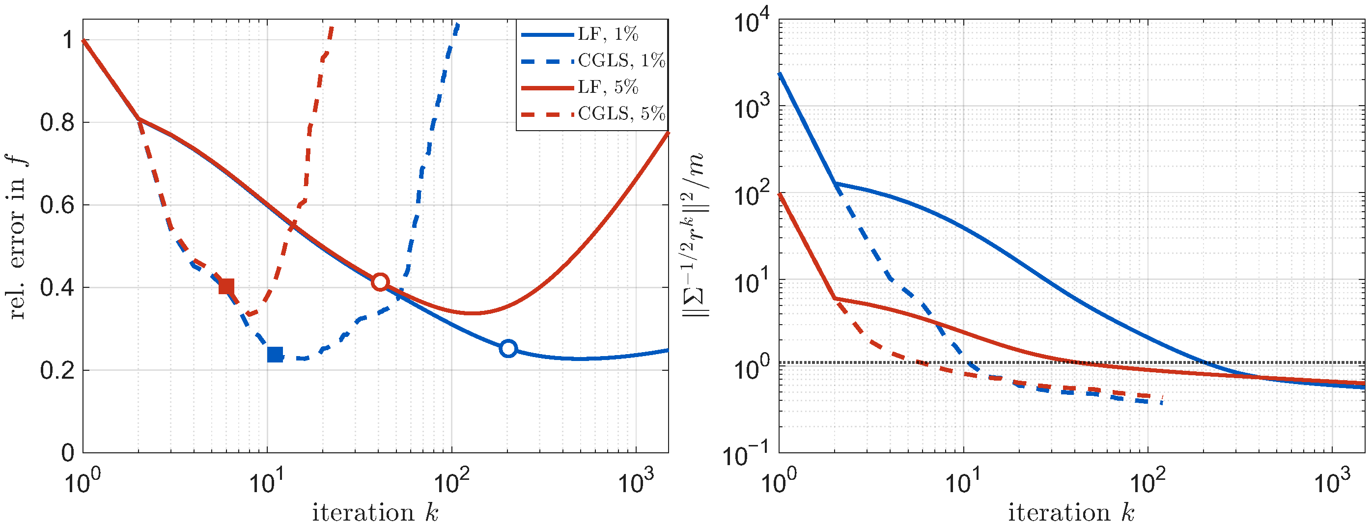Because the conjugate-gradient polynomial adapts to the singular values, the method in practice resolves the informative subspace in a number of iterations comparable to its dimension, the count of singular values above the noise level, rather than the ${(s_1/s_i)}^2$ of Landweber–Fridman. In the experiments, CGLS reaches the discrepancy in 11 iterations rather than 203 at $1\%$ noise, and in 6 iterations rather than 41 at $5\%$ noise (Section 6.2). Like Landweber, CGLS is a regularization method: the iteration index is the regularization parameter, the error semiconverges, and the iteration is stopped by the discrepancy principle (15) [14].

4.4. Similarities and Differences

The three methods differ in the polynomial filter they apply to the singular values, and hence in the number of iterations required, as summarized in

Table 1. Adjoint-based iterative solvers for the least-squares problem (9). Every method costs one forward and one adjoint solve per iteration and is stopped by the discrepancy principle (15); $s_1$ is the largest singular value of ${\mathrm{\Sigma }}^{-1/2}{A}_h$ and $s_{*}$ the smallest one above the noise level. Conjugate gradients trades the dependence on the condition number $s_1/s_{*}$ for a dependence on the effective rank.

Method	Iterations to Reach (15)	Free Parameters
Landweber–Fridman	$O\left({(s_1/s_{*})}^2\right)$	step $\omega$
steepest descent	$O\left({(s_1/s_{*})}^2\right)$	none
conjugate gradient (CGLS/LSQR)	$O\left(\#\{i:s_i\gtrsim s_{*}\}\right)$	none

; steepest descent, which replaces the fixed step $\omega$ of (12) by the locally optimal one but still moves along a single gradient direction, retains essentially the Landweber–Fridman rate.

Landweber’s geometric filter is fixed before the spectrum is seen and damps the slow modes only algebraically; steepest descent takes the locally optimal step but, still searching along a single gradient direction, inherits essentially the same asymptotic rate. The conjugate-gradient method optimizes over the entire Krylov subspace and applies an adaptive degree-k polynomial to the spectrum. For the rapidly decaying, clustered spectra considered here, it reaches the discrepancy in far fewer iterations than Landweber–Fridman. We therefore use CGLS as the deterministic solver and retain the Landweber–Fridman iteration as the historical and conceptual baseline.

The same hierarchy carries over to the statistical formulation of Section 5. There the prior-preconditioned Landweber and conjugate-gradient iterations compute the maximum a posteriori estimate with the identical forward and adjoint solves, and a separate matrix-free Lanczos or randomized eigensolve yields the dominant eigenpairs of the prior-preconditioned Hessian on which the posterior covariance depends (Section 5.4).

5. Statistical Formulation and Uncertainty Quantification

The deterministic solvers of Section 4 return a point estimate and control the noise through early stopping. We now take the Bayesian view in which the same adjoint machinery additionally delivers a calibrated quantification of the uncertainty that the data leave in the reconstruction. We model the noise in (4) as $\epsilon \sim \mathcal{N}(0,\mathrm{\Sigma })$ and place Gaussian priors on the unknowns,

$$f\sim \mathcal{N}(\overline{f},{\mathrm{\Gamma }}_f),u_0\sim \mathcal{N}({\overline{u}}_0,{\mathrm{\Gamma }}_0),$$

(17)

independent of each other and of $\epsilon$, so that $\theta \sim \mathcal{N}(\overline{\theta },\mathrm{\Gamma })$ with $\overline{\theta }=(\overline{f},{\overline{u}}_0)$ and $\mathrm{\Gamma }=diag({\mathrm{\Gamma }}_f,{\mathrm{\Gamma }}_0)$. After discretization $\theta \in {\mathbb{R}}^n$ collects the coefficients of f in a nodal space–time basis together with the values of $u_0$, and $A_h$, $\mathrm{\Gamma }$, $\mathrm{\Sigma }$ are matrices.

5.1. Prior Specification

The prior covariances encode the smoothness expected of the two fields. We use Matérn operators [35,36,37], whose covariance kernel

$$c_{\nu }(z,z^{\prime })={\sigma }^2{\displaystyle \frac{2^{1-\nu }}{\mathrm{\Gamma }\left(\nu \right)}}{\left(\frac{\sqrt{2\nu }\parallel z-z^{\prime }\parallel }{\ell }\right)}^{\nu }{K}_{\nu }\left(\frac{\sqrt{2\nu }\parallel z-z^{\prime }\parallel }{\ell }\right)$$

(18)

is set by a marginal variance ${\sigma }^2$, a correlation length ℓ, and a smoothness index $\nu$ (with $K_{\nu }$ the modified Bessel function and $\mathrm{\Gamma }$ here the gamma function). Three features make this family well suited to the problem. First, the smoothness is explicit: a Matérn-$\nu$ field has sample paths in $C^k$ for every integer $k<\nu -d/2$, so that $\nu >d/2$ already yields continuous realizations and the point observations of Section 2 are almost surely well defined; we take $\nu =5/2$, which gives continuously differentiable draws in one space dimension. Second, the hyperparameters $\sigma$ and ℓ are physically interpretable. Third, through the stochastic partial differential equation representation of Matérn fields [36], the precision ${\mathrm{\Gamma }}^{-1}$ is a sparse elliptic differential operator; this both explains its poor conditioning, which motivates the preconditioning of Section 5.3, and renders the action of ${\mathrm{\Gamma }}^{1/2}$ inexpensive. For the source we use the separable space–time covariance ${\mathrm{\Gamma }}_f={\sigma }_f^2(R_x\otimes R_t)$, where $R_x$ and $R_t$ are unit-marginal-variance Matérn correlation operators with lengths ${\ell }_x$ and ${\ell }_t$. This normalization ensures that the Kronecker product has marginal variance ${\sigma }_f^2$, rather than multiplying the scale once in each factor. For the initial condition, ${\mathrm{\Gamma }}_0$ is a spatial Matérn operator with variance ${\sigma }_0^2$ and length ${\ell }_0$, and ${\overline{u}}_0$ is the known boundary level.

The prior is thus determined by the hyperparameters $\eta =({\sigma }_f,{\ell }_x,{\ell }_t,{\sigma }_0,{\ell }_0)$ together with the noise level in $\mathrm{\Sigma }$. These may be fixed from physical knowledge, as in our experiments, or estimated from the data by empirical Bayes: because the model is linear and Gaussian, the marginal likelihood is available in closed form,

$$p(y\mid \eta )=\mathcal{N}\left(y;A_h\overline{\theta },A_h\mathrm{\Gamma }{A}_h^{\mathrm{\top }}+\mathrm{\Sigma }\right),$$

(19)

and maximizing it over $\eta$ selects the hyperparameters without reference to the truth [38]; the same forward and adjoint solves, and the low-rank structure of Section 5.4, keep each evaluation affordable. Section 6.2.8 quantifies the sensitivity of the errors and credible-band widths to one-at-a-time variations of $({\sigma }_f,{\ell }_x,{\ell }_t,{\sigma }_0)$ around the nominal values, and reports the marginal likelihood (19) that the empirical-Bayes route would maximize.

5.2. The Posterior

With the hyperparameters fixed, Bayes’ theorem gives a posterior density proportional to $exp(-J(\theta \left)\right)$, where

$$J\left(\theta \right)=\frac{1}{2}\parallel {\mathrm{\Sigma }}^{-1/2}(A_h\theta -y){\parallel }^2+\frac{1}{2}{(\theta -\overline{\theta })}^{\mathrm{\top }}{\mathrm{\Gamma }}^{-1}(\theta -\overline{\theta })=\mathrm{\Phi }\left(\theta \right)+\frac{1}{2}{(\theta -\overline{\theta })}^{\mathrm{\top }}{\mathrm{\Gamma }}^{-1}(\theta -\overline{\theta }),$$

(20)

the data misfit $\mathrm{\Phi }$ of (5) augmented by the prior term. Because the forward map is linear, J is quadratic and the posterior is exactly Gaussian, $\theta |y\sim \mathcal{N}({\theta }_{\mathrm{MAP}},H^{-1})$, with

$$H=A_h^{\mathrm{\top }}{\mathrm{\Sigma }}^{-1}{A}_h+{\mathrm{\Gamma }}^{-1}=H_{\mathrm{mis}}+{\mathrm{\Gamma }}^{-1},{\theta }_{\mathrm{MAP}}=\overline{\theta }+H^{-1}{A}_h^{\mathrm{\top }}{\mathrm{\Sigma }}^{-1}\left(y-A_h\overline{\theta }\right),$$

(21)

where $H_{\mathrm{mis}}=A_h^{\mathrm{\top }}{\mathrm{\Sigma }}^{-1}{A}_h$ is the data-misfit Hessian of Section 4.1. No Laplace or Gauss–Newton approximation is involved: H is the exact Hessian of J and (21) is the exact posterior, which are the only approximations entering through the discretization and the low-rank covariance of Section 5.4. Being Gaussian, the posterior mean coincides with the MAP estimate (maximum a posteriori, the mode of the posterior density) (and with the conditional mean), so one linear solve already yields the Bayes estimator.

The exact Gaussian formulas rely on a linear forward map and fixed hyperparameters. For a nonlinear forward model, replacing $A_h$ by the Jacobian gives a Gauss–Newton approximation, whereas the exact Hessian also contains residual-weighted second derivatives; the accuracy of such approximations is not assessed here [27,29]. Unknown hyperparameters may instead be estimated by maximizing the evidence (19); a fully hierarchical treatment would produce a non-Gaussian joint posterior [39,40]. The experiments below remain in the linear fixed-hyperparameter setting.

5.3. Computing the MAP Estimate

The MAP estimate minimizes J and hence solves the regularized normal equations

$$H(\theta -\overline{\theta })=A_h^{\mathrm{\top }}{\mathrm{\Sigma }}^{-1}\left(y-A_h\overline{\theta }\right),H=H_{\mathrm{mis}}+{\mathrm{\Gamma }}^{-1}.$$

(22)

Its gradient $\nabla J\left(\theta \right)=A_h^{\mathrm{\top }}{\mathrm{\Sigma }}^{-1}(A_h\theta -y)+{\mathrm{\Gamma }}^{-1}(\theta -\overline{\theta })$ is, by (8), available from one forward and one adjoint solve, so the adjoint-based iterations of Section 4 carry over to (22) unchanged, now regularized by the prior rather than by early stopping. Gradient descent on J,

$${\theta }^{k+1}={\theta }^k-\omega \left(A_h^{\mathrm{\top }}{\mathrm{\Sigma }}^{-1}\left(A_h{\theta }^k-y\right)+{\mathrm{\Gamma }}^{-1}\left({\theta }^k-\overline{\theta }\right)\right),$$

(23)

is the prior-augmented Landweber iteration and converges to ${\theta }_{\mathrm{MAP}}$ for $0<\omega <2/{\lambda }_{max}\left(H\right)$; preconditioning by the prior covariance yields the better-scaled iteration

$${\theta }^{k+1}={\theta }^k-\omega \left(\mathrm{\Gamma }{A}_h^{\mathrm{\top }}{\mathrm{\Sigma }}^{-1}\left(A_h{\theta }^k-y\right)+{\theta }^k-\overline{\theta }\right),$$

(24)

whose convergence is governed by the spectrum of $I+\tilde{H}$, with

$$\tilde{H}={\mathrm{\Gamma }}^{1/2}{A}_h^{\mathrm{\top }}{\mathrm{\Sigma }}^{-1}{A}_h{\mathrm{\Gamma }}^{1/2}={\mathrm{\Gamma }}^{1/2}{H}_{\mathrm{mis}}{\mathrm{\Gamma }}^{1/2}$$

(25)

the prior-preconditioned data-misfit Hessian. Exactly as in Section 4, this first-order iteration is slow when the data are informative: with ${\lambda }_1={\lambda }_{max}\left(\tilde{H}\right)=3.7\times {10}^6$ in Section 6.2 the per-step contraction factor is $1-2/(2+{\lambda }_1)$, whereas prior-preconditioned conjugate gradients on (22) reaches ${\theta }_{\mathrm{MAP}}$ in a number of solves set by the effective rank [14]. We therefore compute ${\theta }_{\mathrm{MAP}}$ by symmetrically prior-preconditioned conjugate gradients (equivalently, conjugate gradients in prior-whitened coordinates). The dominant eigenpairs of $\tilde{H}$ needed for the posterior covariance are then computed by the separate matrix-free Lanczos or randomized eigensolve described in Section 5.4; the timing table reports this eigensolve as a distinct stage.

5.4. Posterior Covariance and Pointwise Uncertainty

The posterior covariance $H^{-1}$ quantifies the uncertainty that the data leave in $\theta$. Its diagonal yields the pointwise variances of the source and the initial condition, while the off-diagonal blocks give the correlation between the two fields. For the moderate problem sizes considered in this paper, H can be formed and factorized directly, and we do so in order to obtain reference values. At a larger scale, however, one never assembles H explicitly; the structure that makes its inverse accessible is the rapid spectral decay of $\tilde{H}$ in (25).

The action of $\tilde{H}$ on a vector costs one forward and one adjoint solve, together with applications of ${\mathrm{\Gamma }}^{1/2}$. Let ${({\lambda }_i,v_i)}_{i=1}^r$ denote the dominant eigenpairs of $\tilde{H}$, computed by a Krylov or randomized method [27,41]. Writing $V_r=[v_1,\dots ,v_r]$ and $D_r=diag\left({\lambda }_i/(1+{\lambda }_i)\right)$, the Sherman–Morrison–Woodbury identity gives

$$H^{-1}={\mathrm{\Gamma }}^{1/2}{\left(I+\tilde{H}\right)}^{-1}{\mathrm{\Gamma }}^{1/2}\approx \mathrm{\Gamma }-\left({\mathrm{\Gamma }}^{1/2}{V}_r\right)D_r{\left({\mathrm{\Gamma }}^{1/2}{V}_r\right)}^{\mathrm{\top }},$$

(26)

with an error controlled by ${\lambda }_{r+1}$: the directions with ${\lambda }_i\ll 1$ are dominated by the prior and contribute negligibly to the correction. This approximation is optimal, in a well-defined sense, among all rank-r updates of the prior covariance [28], and it underlies large-scale linear Bayesian inversion [26]. The number of eigenvalues above one, 116 in Example 1 and 262 in the two-dimensional example, measures how many directions in the n-dimensional parameter space the data actually inform. The remaining directions, with ${\lambda }_i\ll 1$, span the near-null space of $A_h$ that diffusion and the sparse sampling leave uninformed; there the posterior reverts to the prior, which is precisely what regularizes the reconstruction and what the wide credible bands in those regions report.

The pointwise posterior variance of the fields follows by projecting the coefficient covariance onto the evaluation functionals: for the source at $(x,t)$, $Var\left(f(x,t)|y\right)=\varphi {(x,t)}^{\mathrm{\top }}{\left(H^{-1}\right)}_{ff}\varphi (x,t)$, where $\varphi (x,t)$ is the vector of basis function values, and similarly for $u_0$. An alternative that avoids the eigendecomposition is Hutchinson’s randomized estimator of the diagonal [42], which averages $z\odot H^{-1}z$ over Rademacher probes z and requires one linear solve with H per probe. Its error decays only as $n_s^{-1/2}$ in the number of probes; as shown in Section 6.2, it is therefore far less efficient here than the low-rank approach, which exploits the spectral decay rather than working against it.

5.5. A Calibrated Discrepancy Diagnostic

The whitened discrepancy at the MAP estimate,

$$Q_{\mathrm{MAP}}=\parallel {\mathrm{\Sigma }}^{-1/2}\left(A_h{\theta }_{\mathrm{MAP}}-y\right){\parallel }^2,$$

(27)

is a natural truth-free, prior-predictive check of the model: gross inconsistency between the data and the assumed forward model, noise level, or prior mean inflates it. Its reference distribution requires care. Because ${\theta }_{\mathrm{MAP}}$ is estimated from the same data, $Q_{\mathrm{MAP}}$ is not ${\chi }_m^2$: the fit shrinks the residual in precisely the directions the data inform. The correct null law is available in closed form. Under the joint prior-predictive model, $z=y-A_h\overline{\theta }\sim \mathcal{N}(0,S)$ with $S=A_h\mathrm{\Gamma }{A}_h^{\mathrm{\top }}+\mathrm{\Sigma }$, and (21) gives $A_h{\theta }_{\mathrm{MAP}}-y=-\mathrm{\Sigma }{S}^{-1}z$; whitening z then yields

$$Q_{\mathrm{MAP}}\stackrel{d}{=}{\displaystyle \sum _{i=1}^m}{\displaystyle \frac{{\chi }_{1,i}^2}{1+{\lambda }_i}},\mathbb{E}{Q}_{\mathrm{MAP}}=m-{\displaystyle \sum _{i=1}^m}{\displaystyle \frac{{\lambda }_i}{1+{\lambda }_i}},Var{Q}_{\mathrm{MAP}}=2{\displaystyle \sum _{i=1}^m}{\displaystyle \frac{1}{{(1+{\lambda }_i)}^2}},$$

(28)

a generalized ${\chi }^2$ law, where ${\chi }_{1,i}^2$ are independent and ${\lambda }_i$ are the eigenvalues of ${\mathrm{\Sigma }}^{-1/2}{A}_h\mathrm{\Gamma }{A}_h^{\mathrm{\top }}{\mathrm{\Sigma }}^{-1/2}$, equivalently, the nonzero spectrum of (25) padded with zeros. These moments are byproducts of the low-rank spectrum. With only its leading $r<m$ eigenvalues retained and the omitted eigenvalues approximated by zero, we use

$${\mu }_r=m-{\displaystyle \sum _{i=1}^r}{\displaystyle \frac{{\lambda }_i}{1+{\lambda }_i}},v_r=2\left[(m-r)+{\displaystyle \sum _{i=1}^r}{\displaystyle \frac{1}{{(1+{\lambda }_i)}^2}}\right].$$

The $(m-r)$ term retains the unresolved directions. We flag misspecification when $Q_{\mathrm{MAP}}>{\mu }_r+2.58\sqrt{v_r}$, using the normal approximation to (28); the reported flags lie well beyond this threshold. This diagnostic does not alter the discrepancy stopping rule (15), which is calibrated to the noise residual of the true parameter.

5.6. Summary: The Reconstruction and Uncertainty-Quantification (UQ) Algorithm

Algorithm 1 collects the complete procedure used in the experiments. Every step accesses the heat equation only through the forward and adjoint solves of Section 3; no operator is assembled, and the dominant cost is the $O\left(r\right)$ forward/adjoint pairs of the eigenvalue computation.

Algorithm 1 Adjoint-based MAP reconstruction and Gaussian uncertainty quantification for the joint source and initial-condition problem.

Input: data y; noise covariance $\mathrm{\Sigma }$; prior mean $\overline{\theta }$ and covariance $\mathrm{\Gamma }$ (hyperparameters $\eta$ fixed or set by empirical Bayes); forward and adjoint solvers for $A_h$ and $A_h^{\mathrm{\top }}$. 1. (Optional) hyperparameters. Maximize the closed-form evidence (19) over $\eta$ (empirical Bayes). 2. MAP estimate. Solve $H(\theta -\overline{\theta })=A_h^{\mathrm{\top }}{\mathrm{\Sigma }}^{-1}(y-A_h\overline{\theta })$ by symmetrically $\mathrm{\Gamma }$-preconditioned conjugate gradients (one forward and one adjoint solve per step) to obtain ${\theta }_{\mathrm{MAP}}$. 3. Dominant spectrum. Compute the leading eigenpairs ${({\lambda }_i,v_i)}_{i=1}^r$ of $\tilde{H}={\mathrm{\Gamma }}^{1/2}{H}_{\mathrm{mis}}{\mathrm{\Gamma }}^{1/2}$ by a matrix-free Lanczos or randomized method, with r chosen so that ${\lambda }_{r+1}\ll 1$. 4. Posterior covariance. Form $H^{-1}\approx \mathrm{\Gamma }-\left({\mathrm{\Gamma }}^{1/2}{V}_r\right)D_r{\left({\mathrm{\Gamma }}^{1/2}{V}_r\right)}^{\mathrm{\top }}$ with $D_r=diag\left({\lambda }_i/(1+{\lambda }_i)\right)$ [Equation (26)]. 5. Model check. Evaluate the whitened discrepancy $Q_{\mathrm{MAP}}={\parallel {\mathrm{\Sigma }}^{-1/2}(A_h{\theta }_{\mathrm{MAP}}-y)\parallel }^2$ and refer it to its prior-predictive null law (28). With the rank-r spectrum of step 3 and the omitted eigenvalues approximated by zero, use ${\mu }_r=m-{\sum }_{i=1}^r{\lambda }_i/(1+{\lambda }_i)$ and $v_r=2[(m-r)+{\sum }_{i=1}^r{(1+{\lambda }_i)}^{-2}]$; flag misspecification when $Q_{\mathrm{MAP}}>{\mu }_r+2.58\sqrt{v_r}$. 6. Pointwise uncertainty. For each $(x,t)$ form $Var\left(f(x,t)\mid y\right)=\varphi {(x,t)}^{\mathrm{\top }}{\left(H^{-1}\right)}_{ff}\varphi (x,t)$, and analogously for $u_0$. Output: MAP estimate ${\theta }_{\mathrm{MAP}}$; pointwise posterior standard deviations; and ${\theta }_{\mathrm{MAP}}\pm 1.96\mathrm{sd}$ credible bands. Every step uses only forward and adjoint solves of the heat equation.

6. Numerical Experiments

6.1. Setup and Verification

In Examples 1 and 2, we set $D=(0,0.2)$ m, $T=10$ s and $\kappa ={10}^{-3} {\mathrm{m}}^2/\mathrm{s}$. The forward problem is discretized with $N_x=60$ intervals ($\mathrm{\Delta }x\approx 3.3$ mm) and $N_t=200$ Crank–Nicolson steps ($\mathrm{\Delta }t=0.05$ s). Six sensors are placed at $x=0.03,0.06,\dots ,0.18$ m and sampled at every second time step, including $t=0$, which gives $m=606$ observations. The source is represented on a bilinear nodal basis with 30 nodes in space and 41 in time ($n_f=1230$ coefficients), and the initial condition is represented by its values at the 59 interior grid nodes, so that $n=1289$. The boundary temperature is held at 20 K above ambient at both ends. The priors are of Matérn-5/2 type: for the source, a separable covariance with standard deviation 1.5 K/s and correlation lengths 0.03 m and 1.5 s; for the initial condition, standard deviation 1 K, correlation length 0.05 m, and mean equal to the boundary value of 20 K. These values reflect the physical setting: the correlation lengths are of the order of the expected width of a heating event and of the sensor spacing, and the marginal standard deviations of the expected source amplitude and initial-state uncertainty; their influence is quantified in Section 6.2.8. The noise is independent and identically distributed (i.i.d.) Gaussian, $\mathrm{\Sigma }={\sigma }^{2}I$, with $\sigma$ set to 1% of the dynamic range of the clean data unless stated otherwise ($\sigma =0.019$ K in Example 1). All computations were performed in MATLAB; wall-clock times are collected in Section 6.5.

Before any inversion, we verify the underlying machinery. The adjoint identity $\langle A_h\theta ,w\rangle =\langle \theta ,A_h^{\mathrm{\top }}w\rangle$ (in the Euclidean coefficient inner products of Section 3) holds with relative error below $5\times {10}^{-15}$ over random probes, and the matrix-free maps agree with an independently assembled matrix $A_h$ to the same precision. Central finite differences of the objective (20) match the adjoint gradient with relative error $9\times {10}^{-11}$ at step $h={10}^{-3}$, which is consistent with the accuracy floor of second-order differences in double precision. The preconditioned iterations converge to the closed-form MAP estimate (21), and the credible intervals are verified by the coverage experiment described below.

6.2. Example 1: Deterministic Versus Bayesian Reconstruction

The true source is the separable Gaussian pulse $f^{†}(x,t)=2exp\left(-{(x-0.12)}^2/(2·0.{02}^2)\right)exp\left(-{(t-4)}^2/(2·1^2)\right)$ K/s, and the true initial condition is the parabola $u_0^{†}\left(x\right)=20+5(x/L)(1-x/L)$ K, which deviates from the prior mean by up to 1.25 K. Figure 1 displays the configuration and the data. We contrast the deterministic reconstruction, a point estimate from the data misfit alone, regularized by early stopping (Section 4), with the Bayesian reconstruction, which adds the prior and returns calibrated uncertainty (Section 5).

6.2.1. Deterministic Reconstruction

The deterministic estimate minimizes the data misfit (9) by the Landweber–Fridman and conjugate-gradient (CGLS) iterations of Section 4, started from $f\equiv 0$, $u_0\equiv 20$ and stopped by the discrepancy principle (15). Both exhibit the classical semiconvergence (Figure 2): the source error first falls and then rises as the iteration begins to fit the noise. The two methods differ sharply in cost. At 1% noise the Landweber–Fridman iteration reaches the discrepancy only at $k_{*}=203$, whereas conjugate-gradient least squares reaches it at $k_{*}=11$; at 5% noise, the counts are 41 and 6. Conjugate gradients thus attains the same discrepancy and a comparable source error, 0.24 at 1% and 0.40 at 5% noise, in roughly an order of magnitude fewer forward and adjoint solves. The initial condition is recovered to about 1% relative error in both cases, reflecting its direct observation at $t=0$.

6.2.2. Bayesian Reconstruction

Adding the Gaussian priors of Section 5.1 and computing the posterior (21) lowers the source error to 0.12 (about half the deterministic value at the same noise level) and the initial-condition error to 0.002. The smoothness prior removes the oscillatory artifacts that early stopping leaves in the deterministic estimate, as Figure 3 and Figure 4 show. Beyond the improved point estimate, the Bayesian formulation supplies pointwise credible bands, which behave as the sensor geometry dictates: narrow for the initial condition everywhere, narrow for the source near the sensors (hence across the well-instrumented region in which the pulse happens to lie), and wide near the spatial boundaries, which the sensors barely observe; the widening at the temporal ends of the source window is mild because the observations extend to $t=T$ and the prior correlates the source in time. For fixed $A_h$, $\mathrm{\Gamma }$, and $\mathrm{\Sigma }$ the posterior covariance is independent of the observed data, so the bands narrow where the forward operator and the prior make the data informative, not because a source is present there. The posterior standard deviation field of Figure 3 renders the sensor geometry directly visible.

Figure 4 displays the two estimates against the truth along two time slices and for the initial condition. The discrepancy-stopped deterministic estimate (orange, dashed) oscillates around the truth: at the stopping index the iteration has recovered the singular directions the data resolve and left the rest at zero, and this near-truncation of the spectrum rings around the pulse, much as a truncated singular-value expansion would (the conjugate-gradient filter factors are adaptive polynomials, close to one on the resolved directions and close to zero on the rest, not an exact 0–1 cutoff). It is nevertheless the correct benchmark, fitting the data to the discrepancy tolerance (15) while using no prior beyond the stopping rule. The posterior mean replaces the truncation by the smooth spectral weights ${\lambda }_i/(1+{\lambda }_i)$ of (26), suppressing the ringing, and its 95% band, narrow near sensors and wide toward the domain corners, prices the undetermined directions. The initial condition (right panel) is recovered accurately by both, being observed directly at $t=0$; only the Bayesian band certifies this without reference to the truth.

6.2.3. Convergence to the MAP Point

We compared the preconditioned first-order iteration (24) with preconditioned conjugate gradients, both matrix-free at one forward and one adjoint solve per step. With ${\lambda }_1=3.7\times {10}^6$, the first-order method contracts by roughly $1-5\times {10}^{-7}$ per step in the worst direction and reaches a relative error of $6\times {10}^{-2}$ after 600 steps, whereas conjugate gradients reaches $2\times {10}^{-7}$ in the same number of forward/adjoint solve pairs. The practical implication is that the adjoint structure of the Landweber–Fridman method carries over to the statistical setting unchanged, but the fixed-point iteration itself should be replaced by a Krylov method once a prior term is present.

6.2.4. Low-Rank Posterior Covariance

Figure 5 shows the eigenvalues of $\tilde{H}$: they fall below one near index 117 and decay by thirteen orders of magnitude within the first 500 indices, so that the data inform roughly 116 of the 1289 directions. Truncating (26) at rank 120 reproduces the pointwise variances with a median relative error of $1.8\times {10}^{-3}$, and rank 160 reaches $5.9\times {10}^{-5}$. By contrast, Hutchinson’s estimator still has a median relative error of 0.18 after 1000 probe solves and follows the $n_s^{-1/2}$ rate: a budget three orders of magnitude costlier in time than the low-rank route while still more than three orders of magnitude less accurate, and matching $5.9\times {10}^{-5}$ at that rate would take $1000\times {\left(0.18/(5.9\times {10}^{-5})\right)}^2\approx {10}^{10}$ probes (each probe requires a full linear solve with H; in wall-clock terms, ten measured probes take 16 s, extrapolating to $\approx 1.6\times {10}^3$ s for 1000, against 1.2 s for the rank-160 route; Section 6.5). When the spectrum decays in this manner, the eigendecomposition is clearly the more appropriate tool.

To perform an end-to-end verification of the linear-Gaussian implementation, we drew 300 parameter vectors from the prior, simulated data for each, and computed the corresponding posterior. Across the 1289 parameter components, the pointwise 95% credible intervals attained a mean empirical coverage of 0.9496, with componentwise coverage ranging from 0.910 to 0.980, consistent with binomial variation at 300 replicates. Robustness to prior misspecification is examined next.

6.2.5. Coverage Under Prior Misspecification and a Discontinuous Source

We assess prior misspecification, with the prior, sensors, and noise level ($\sigma =0.019$ K) of Example 1 held fixed. We first consider the discontinuous source

$$f^{†}(x,t)=2{\mathbf{1}}_{\left\{\right|x-0.12|\le 0.02\}}{\mathbf{1}}_{\{3\le t\le 5\}}\mathrm{K}/\mathrm{s},$$

which violates the smoothness assumption of the Matérn-5/2 prior while leaving the forward problem linear. The posterior mean recovers the location and magnitude of the block but smooths its edges, giving a relative source error of 0.41, compared with 0.43 for the deterministic estimate. Although the pointwise 95% bands cover 96.3% of the full space–time grid, their coverage falls to 0.63 over the block and 0.03 within one grid cell of its boundary, where the smoothing bias is concentrated (Figure 6).

The normalized discrepancy is $Q_{\mathrm{MAP}}/m=1.00$. Its prior-predictive null distribution (28) has normalized mean 0.81 and standard deviation 0.051, placing the observed value approximately 3.8 standard deviations above the null mean and above the calibrated threshold $0.81+2.58\left(0.051\right)\approx 0.94$. By contrast, the inappropriate ${\chi }_m^2$ threshold $1+2.58\sqrt{2/m}\approx 1.15$ would not flag the misspecification. The discrepancy is nevertheless much smaller than the value of approximately 53 in Section 6.3, indicating that the diagnostic is more sensitive to forward-model inconsistency than to prior mismatch in weakly informed directions.

We next repeat the experiment over 300 realizations from each of two out-of-prior ensembles: narrow pulses, with random amplitudes in $[1,3]$ K/s, random locations, and widths $s_x\in [8,15]$ mm and $s_t\in [0.3,0.8]$ s; and discontinuous blocks of the form above. These scales are smaller than the prior correlation lengths ${\ell }_x=30$ mm and ${\ell }_t=1.5$ s. Because these truths need not lie in the source basis span, coverage is evaluated on the space–time grid rather than for the basis coefficients.

Table 2. Coverage under prior misspecification for 300 replicates per ensemble, with the nominal prior and $\sigma =0.019$ K fixed. The columns report the mean (minimum) field-level coverage of the pointwise $95\%$ bands for f, the mean coverage for $u_0$, the mean normalized discrepancy $Q_{\mathrm{MAP}}/m$, and the fraction exceeding the calibrated MAP-residual threshold $0.94$ from (28).

Truth Ensemble	Coverage f, Mean (min)	Coverage ${\mathit{u}}_0$	Discrepancy/m	Flag Rate
prior draws (reference)	0.950 (0.79)	0.952	0.80	0.01
narrow pulses	0.996 (0.97)	0.995	0.79	0.00
discontinuous blocks	0.957 (0.91)	0.995	0.97	0.53

reports a mean field-level coverage of 0.950 for the prior-drawn reference, 0.996 for the narrow pulses, and 0.957 for the blocks. The high aggregate values partly reflect that the compact sources are zero or negligible over most of the domain. For the block ensemble, mean coverage restricted to the active support is only 0.48 and falls to 0.11 within one grid cell of the discontinuity. The calibrated discrepancy diagnostic flags none of the narrow-pulse realizations and 53% of the block realizations, compared with 1% of the prior draws. Thus, global coverage can mask substantial local undercoverage near sharp interfaces. When such interfaces are expected, an edge-preserving prior, such as a Besov or hierarchical prior [23,25], is more appropriate, at the cost of losing the exact Gaussian posterior.

6.2.6. Effect of the Noise Level

Table 3. Example 1: relative $L^2$ reconstruction errors of the deterministic (CGLS, discrepancy-stopped) and the Bayesian (MAP) estimate at four noise levels.

Noise Level	0.5%	1%	2%	5%
$\sigma$ (K)	0.0095	0.019	0.038	0.095
deterministic, f	0.208	0.219	0.266	0.414
deterministic, $u_0$	0.012	0.013	0.012	0.013
Bayesian, f	0.086	0.119	0.187	0.371
Bayesian, $u_0$	0.002	0.003	0.002	0.004

and the left panel of Figure 7 report the reconstruction errors of both methods for noise between 0.5% and 5% of the data range, at a fixed realization per level. The Bayesian source error is about half the deterministic one at the lower noise levels (ratios 0.41 at 0.5% and 0.53 at 1%), the advantage narrowing as the noise grows (0.70 at 2% and 0.90 at 5%, where the heavily regularized deterministic estimate is nearly as accurate); the gap on the initial condition is larger still: the prior, together with the direct observation at $t=0$, holds $u_0$ to ∼${10}^{-3}$ relative error, whereas the unregularized deterministic estimate stalls near ${10}^{-2}$. Both source errors grow sublinearly: over the tenfold noise increase, the deterministic error roughly doubles, while the Bayesian error grows by about a factor of four.

6.2.7. Effect of Numerical Error

We probe the influence of the discretization by generating the data on a fine mesh ($N_x=240$, $N_t=800$) and inverting them on a sequence of coarser meshes, so that no inverse crime is committed: inverting data with the same discretization that generated them would artificially remove the forward-model error. The right panel of Figure 7 shows the result. The Bayesian source error is essentially flat ($\approx 0.12$) from $N_x=20$ to 120: the prior supplies a mesh-independent, scale-selective regularization, so refining the grid neither helps nor harms. The deterministic error, by contrast, is markedly discretization-sensitive (about 0.16 at $N_x=40$ but rising to 0.33 at $N_x=120$) because early stopping does not control the finer parameter modes that refinement introduces, and the iteration expends its budget fitting noise into them. Inverting data generated on the same mesh (the inverse crime, crosses in Figure 7) changes the deterministic error by less than 0.01, confirming that the Crank–Nicolson model resolves the forward problem well enough that the fine-mesh data are honest: the discretization sensitivity is a property of the regularization, not of the forward solver. Figure 7 summarizes both studies. In the left panel the initial-condition curves are flat across the noise range, since $u_0$ is observed directly at $t=0$, and the Bayesian advantage on the source is a factor of about two at moderate noise, narrowing at 5% (Table 3); each level uses a single fixed noise realization, so the precise ratios carry sampling variability; in the right panel the monotone rise of the deterministic curve under refinement, against the flat Bayesian one, is the practical warning of this section: for discrepancy-stopped iterations the discretization acts as an implicit regularization parameter, so refining the mesh without strengthening the regularization degrades the reconstruction.

6.2.8. Sensitivity to the Prior Hyperparameters

The hyperparameters $\eta =({\sigma }_f,{\ell }_x,{\ell }_t,{\sigma }_0)$ were fixed in Section 6.1 based on physical considerations, with the correlation lengths, in particular, controlling how aggressively the prior smooths the source. To quantify the dependence we repeat the Bayesian reconstruction of Example 1 with each hyperparameter halved and doubled, relative to its nominal value, one at a time, with the data, noise, and other hyperparameters fixed.

Table 4. Example 1, $1\%$ noise: sensitivity of the Bayesian reconstruction to one-at-a-time variations of the prior hyperparameters about their nominal values (${\sigma }_f=1.5$ K/s, ${\ell }_x=0.03$ m, ${\ell }_t=1.5$ s, ${\sigma }_0=1$ K; ${\ell }_0=0.05$ m fixed). Columns: relative $L^2$ errors of the posterior mean, mean $95\%$ band widths, and the log marginal likelihood (19).

Prior Setting	Error f	Error ${\mathit{u}}_0$	Band f (K/s)	Band ${\mathit{u}}_0$ (K)	$log\mathit{p}\left(\mathit{y}\right|\mathit{\eta })$
nominal	0.119	0.002	1.214	0.313	1269.6
${\ell }_x\times \frac{1}{2}$	0.115	0.002	2.525	0.325	1267.5
${\ell }_x\times 2$	0.134	0.002	0.431	0.300	1292.2
${\ell }_t\times \frac{1}{2}$	0.170	0.002	1.223	0.333	1183.9
${\ell }_t\times 2$	0.090	0.002	1.207	0.299	1334.2
${\sigma }_f\times \frac{1}{2}$	0.100	0.002	0.622	0.299	1325.4
${\sigma }_f\times 2$	0.146	0.002	2.402	0.333	1198.5
${\sigma }_0\times \frac{1}{2}$	0.120	0.002	1.213	0.197	1272.1
${\sigma }_0\times 2$	0.119	0.002	1.215	0.499	1263.6

reports the source and initial-condition errors, the mean 95% band width for each field, and the log marginal likelihood (19) that the empirical-Bayes route of Section 5.1 would maximize.

The source error stays between 0.090 and 0.170 across the eight perturbed settings, against 0.119 nominal—at most a factor of about 1.4 under any twofold change—and the initial-condition error remains 0.002 throughout, so the reconstruction is stable and not an artifact of a prior tuned to the truth, ${\ell }_t$ being the most influential parameter. The band widths respond as the prior dictates, scaling with the marginal variances (mean 95% band for f from 0.62 to 2.40 K/s across ${\sigma }_f$, for $u_0$ from 0.20 to 0.50 K across ${\sigma }_0$) and widening as ${\ell }_x$ shortens (2.53 against 0.43 K/s), which makes explicit that credible bands are conditional on the prior scales. The evidence ranks the settings usefully: its two largest values, at ${\ell }_t\times 2$ and ${\sigma }_f\times \frac{1}{2}$, are precisely the two smallest source errors (0.090 and 0.100), both better than nominal. The one-at-a-time evidence thus broadly tracks the reconstruction quality, suggesting that empirical-Bayes maximization of (19)—a joint optimization we have not performed—may improve on the physically chosen values. This is an indication from the one-at-a-time study, not an established consequence of joint evidence maximization; we recommend empirical Bayes when physical knowledge is weak, while full propagation of hyperparameter uncertainty lies beyond the present study.

6.3. Example 2: Two-Component Source and an Initial Condition Offset

The second example mimics an experiment in which the nominal initial state is known only up to a uniform offset, a common situation when sensors are calibrated to relative rather than absolute temperature. The true source is a sum of two Gaussian pulses, located at $(x,t)=(0.07\mathrm{m},2.5\mathrm{s})$ with amplitude 1.5 K/s and at $(0.14\mathrm{m},6\mathrm{s})$ with amplitude 2 K/s. The true initial condition is the nominal parabolic profile of Example 1 shifted by $c^{†}=1.5$ K, and the unknowns are the source coefficients together with the scalar offset c, to which we assign the prior $c\sim \mathcal{N}(0,2^2)$. The noise level is 1% ($\sigma =0.023$ K).

Joint estimation recovers the offset as $c=1.500\pm 0.008$ K and the source with relative error 0.25, and the normalized discrepancy at the MAP point is 0.83, in agreement with its null expectation of 0.83 for this configuration (Section 5.5). Fixing $c=0$ instead, as a deterministic formulation with a trusted initial state would do, drives the source error to 2.81: the inversion fabricates a strong spurious source sheet at early times near the boundaries in order to mimic the missing initial heat, as is clearly visible in the third panel of Figure 8. The statistical formulation flags this problem without reference to the truth, since the normalized discrepancy of the misspecified fit is approximately 53, three orders of magnitude beyond the spread of the null law of Section 5.5 (mean 0.83, standard deviation 0.05). The discrepancy diagnostic is thus a model-error indicator, and the joint formulation removes the bias at the cost of one additional scalar parameter.

6.4. Example 3: A Two-Dimensional Plate

To confirm that the framework and its uncertainty quantification carry over to higher dimensions, we repeat the joint reconstruction on a rectangular plate $\mathrm{\Omega }=(0,0.2)\times (0,0.1)$ m with homogeneous Dirichlet conditions, discretized by $N_x=40$ and $N_y=20$ cells and $N_t=80$ Crank–Nicolson steps (741 interior nodes). The true source is a localized space–time pulse centered at $(0.12,0.05)$ m and $t=4$ s, and the true initial condition is the smooth interior bump $u_0^{†}=5sin(\pi x/L_x)sin(\pi y/L_y)$ K; both are unknown. Temperatures are recorded at a $6\times 4$ grid of 24 interior sensors, sampled at every second step including $t=0$, giving $m=984$ observations of a parameter of dimension $n=1326$ (a $9\times 5\times 13$ nodal source basis together with the initial condition on the interior grid). The priors are of Matérn-5/2 type as before, and the discrete adjoint again satisfies the identity ${\langle A_h\theta ,w\rangle }_{{\mathbb{R}}^m}={\langle \theta ,A_h^{\mathrm{\top }}w\rangle }_{{\mathbb{R}}^n}$ to machine precision.

The reconstructions of Figure 9 reproduce the one-dimensional picture. The deterministic CGLS estimate, stopped by the discrepancy principle at $k_{*}=8$, recovers the source to relative error 0.41 but leaves the initial condition essentially unrecovered away from the sensors (relative error 0.97), because the data constrain $u_0$ only at the few observation points. The Bayesian posterior mean is more accurate on both fields (source error 0.38 and initial-condition error 0.08) because the smoothness prior fills in the unobserved interior, and it additionally supplies the pointwise standard-deviation fields of the right-hand panels, which narrow near the sensors (the source region being well instrumented) and widen where the plate is poorly observed. The prior-preconditioned data-misfit Hessian retains its rapid spectral decay, with ${\lambda }_1=4.5\times {10}^5$ and the eigenvalues falling below one at index 263: of the 1326 parameter directions, only about 262 are informed by the data, so the low-rank covariance of Section 5.4 is as effective in two dimensions as in one. Every step uses the same forward and adjoint solves, now of the two-dimensional heat equation. The pipeline is inexpensive at this resolution: the deterministic reconstruction takes 0.07 s, the matrix-free MAP estimate 3.3 s, and 300 dominant eigenpairs with the pointwise variances a further 2.7 s (

Table 5. Wall-clock times (s) for the deterministic reconstruction, the MAP solve, the posterior uncertainty quantification, and the complete Bayesian pipeline. The posterior-UQ time includes the low-rank covariance computation and pointwise variance projection.

Example	Deterministic CGLS	MAP	Posterior UQ	Total Bayesian
1 (1D, $n=1289$, $m=606$)	0.04	1.4	1.2	2.6
2 (1D offset, $n=1231$, $m=606$)	–	0.3	–	0.3
3 (2D, $n=1326$, $m=984$)	0.07	3.3	2.7	6.0

), the matrix-free quantities agreeing with the dense reference to ${10}^{-5}$ or better. We emphasize the scope: with $n=1326$ unknowns this example shows that the formulation, the discrete adjoint, and the low-rank uncertainty quantification transfer unchanged to $d=2$, not that the pipeline has been exercised at large scale; the ingredients required at ${10}^5$–${10}^6$ parameters (finite element discretizations, mesh-independent prior operators, randomized eigensolvers) are established in the literature [26,27,28] and not re-demonstrated here.

6.5. Computational Cost

Table 5 reports the wall-clock times for the deterministic reconstruction, the MAP solve, the posterior uncertainty quantification, and the complete Bayesian pipeline. Example 2 uses a direct posterior computation, so its MAP and uncertainty-quantification costs are included in a single reported time. All runs used MATLAB R2025b on two threads of an Intel Core i7-1355U (1.70 GHz, 16 GB RAM). The complete Bayesian pipeline costs 2.6 s in Example 1 and 6.0 s for the plate; the Hutchinson timing comparison is reported in Section 6.2.

7. Conclusions

The contributions of this work are fourfold. First, a single adjoint solve of the heat equation yields the misfit gradient with respect to both an internal space–time source and the initial temperature—the adjoint state in the interior and its trace at $t=0$—so the joint reconstruction costs no more per iteration than the source-only problem, whereas existing joint procedures were restricted to spacewise-dependent sources from temperature snapshots. Second, on this gradient we build a unified framework in which a deterministic estimate (conjugate-gradient least squares stopped by the statistical discrepancy principle) and a Bayesian estimate (the MAP point of an exactly Gaussian posterior, by prior-preconditioned conjugate gradients) share the identical forward and adjoint machinery, with Landweber–Fridman retained as a baseline. Third, the framework delivers an exact finite-dimensional Gaussian posterior with verifiable uncertainty at the cost of forward and adjoint solves alone: the low-rank identity (26) converts the rapid spectral decay of the prior-preconditioned data-misfit Hessian into pointwise credible bands, and the exact discrete adjoint makes the pipeline verifiable, with the bands attaining nominal coverage over prior-drawn truths (prior-predictive calibration). Fourth, the whitened MAP discrepancy, referred to as its exact prior-predictive generalized-${\chi }^2$ null law (28)—itself a byproduct of the low-rank spectrum—serves as a truth-free, prior-predictive model-error indicator, detecting both a misspecified initial condition that a least-squares fit silently absorbs into the source and a discontinuous source that violates the prior.

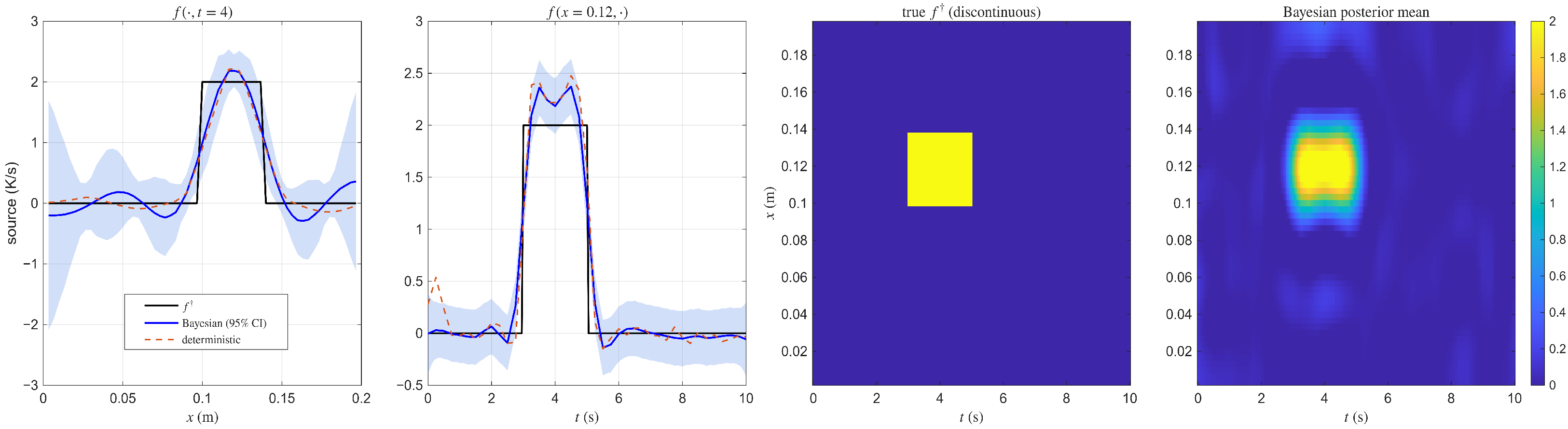
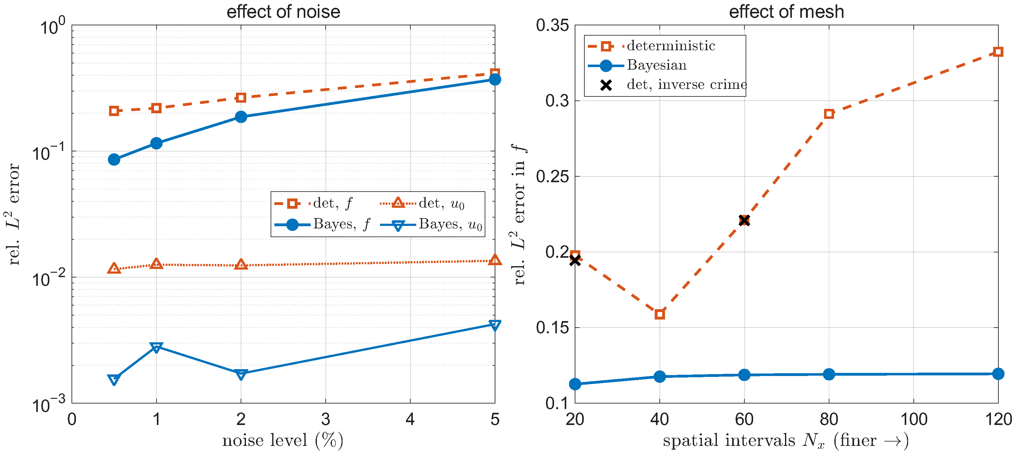
The experiments support these contributions while marking their limits. Conjugate gradients is substantially faster than the Landweber baseline, and the Bayesian reconstruction is more robust to noise and mesh refinement. Prior-predictive coverage is nominal, whereas the out-of-prior experiments show that uncertainty failures concentrate near sharp interfaces; the discrepancy diagnostic detects consequential model mismatch but is less sensitive to features weakly informed by the data. The sensitivity and two-dimensional studies support robustness and dimensional transfer at the moderate scales tested here.

We close with the natural extensions, distinguishing what has been demonstrated from what has not. The experiments are one- and two-dimensional with at most 1326 unknowns; at a larger scale, the required ingredients—finite element discretizations, mesh-independent prior operators, randomized matrix-free eigensolvers—are established [26,27,28], and their integration here is a natural next step we have not exercised; discrete-adjoint consistency also needs care under adaptive time stepping. Treating the diffusivity as uncertain renders the problem nonlinear (unknown additive boundary data, by contrast, enter affinely and would remain within the linear Gaussian framework as a third unknown) and the posterior non-Gaussian; a Laplace or Gauss–Newton approximation about the MAP point is then available, whose accuracy is not addressed by the present linear experiments and would need a dedicated assessment against sampling or ensemble methods [43,44]. Sources with sharp interfaces are better served by edge-preserving than Matérn priors—as the discontinuous-source experiment makes this quantitative—at the price of the exact Gaussian posterior. Finally, joint inference of noise and prior hyperparameters would relax the fixed-hyperparameter assumption but lies beyond the present study.