A State-Space Agent-Based Model for Infectious Disease Spread

Abstract

We present a novel framework for epidemiological disease spread modeling that combines agent-based simulation with Boolean state-space representations and optimal filtering for state estimation under noisy observations. Our approach models individual agents in discrete Susceptible-Exposed-Infected-Recovered (SEIR) states using a compact 2-bit Boolean representation, with agent interactions governed by scheduled contact patterns. To address the challenge of inferring latent infection states from limited and noisy testing data, we develop two complementary inference approaches: (1) a Boolean Kalman particle filter for small populations that tracks the full joint distribution over agent states, and (2) a mean-field approximation for large populations that factorizes the posterior into independent marginal distributions, enabling scalability to realistic population sizes. Unlike continuous-state Kalman filters, our methods naturally handle the discrete nature of epidemiological states while accommodating realistic observation models where only a subset of agents are tested at each time step, with test results subject to false positive and false negative errors. We demonstrate that this framework enables accurate reconstruction of population-level infection dynamics and individual agent states from sparse, noisy observations across populations from 100 to 50,000 agents, providing a computationally tractable approach for real-time epidemic monitoring.

1. Introduction

The COVID-19 pandemic has underscored the critical need for accurate, real-time epidemiological modeling frameworks capable of tracking disease spread through populations despite limited and imperfect surveillance data [1]. Traditional compartmental models (e.g., Susceptible-Infected-Recovered (SIR), Susceptible-Exposed-Infected-Recovered (SEIR)) provide valuable insights into aggregate disease dynamics but lack the granularity to capture individual-level heterogeneity in contact patterns, testing behavior, and infection progression [2]. Conversely, agent-based models (ABMs) offer rich microscopic detail but face significant challenges in state estimation: how can we infer the true infection states of thousands of individuals when we observe only noisy test results from a small subset?

This paper addresses this fundamental inference problem by developing a state-space framework that combines the representational power of agent-based models with the statistical rigor of optimal filtering theory. Our key innovation lies in recognizing that epidemiological states are inherently discrete and can be efficiently represented using Boolean variables, enabling the application of Boolean Kalman filtering techniques originally developed for gene regulatory networks [3]. However, while particle filtering is asymptotically exact as the number of particles grows [4], the curse of dimensionality makes straightforward particle filtering impractical in high-dimensional epidemic ABMs [5], motivating scalable mean-field approximations for realistic population sizes [6].

1.1. Motivation and Challenges

Real-world epidemic surveillance presents several distinct challenges:

• Partial observability: Only a fraction of the population is tested at any given time, leaving most infection states latent.
• Noisy measurements: Diagnostic tests exhibit false positive and false negative rates, corrupting observations with measurement error.
• Discrete states: Epidemiological compartments (S, E, I, R) are categorical, not continuous quantities.
• Nonlinear dynamics: Disease transmission depends on complex, nonlinear interactions between agents.
• High dimensionality: Tracking individual-level states in large populations creates computational challenges that grow exponentially with population size.

Standard Kalman filtering assumes continuous Gaussian states and linear dynamics, making it unsuitable for this domain. Extended and unscented Kalman filters can handle nonlinearity but still assume continuous state spaces. Particle filters offer a general solution for nonlinear, non-Gaussian problems, but become computationally prohibitive in high dimensions without careful design or approximations.

1.2. Our Approach

We propose a Boolean state-space agent-based model (BS-ABM) where each agent’s SEIR state is encoded using 2 Boolean variables, yielding four possible states: $\{00,10,11,01\}\equiv \{S,E,I,R\}$. Agent interactions follow predefined schedules (e.g., workplace, household, social contacts), and state transitions are governed by probabilistic rules that depend on contact with infected individuals. For state estimation, we develop two complementary approaches tailored to different population scales:

Small Populations (Particle Filter): For populations up to approximately 100 agents, we adapt the Auxiliary Particle Filter implementation of the Boolean Kalman Filter (APF-BKF) framework of Imani and Braga-Neto [3] to the epidemiological setting. This approach maintains a population of particles, each representing a hypothesis about all agents’ Boolean states, and propagates these through the discrete-state transition dynamics while updating particle weights based on noisy observations. While the state space of $4^{100}\approx {10}^{60}$ configurations is enormous, particle filtering provides an effective approximation that captures dependencies between agent states arising from their contact structure.

Large Populations (Mean-Field Approximation): For populations of $N\gg 100$ agents, the state space of $4^N$ configurations renders particle filtering utterly intractable—no practical number of particles can meaningfully sample this space. We, therefore, employ a mean-field approximation that factorizes the posterior distribution into independent marginal distributions for each agent. Instead of tracking the full joint distribution $p\left({\mathbf{X}}_k\right|{\mathbf{Y}}_{1:k})$, we maintain N separate marginal distributions $p\left(X_k^{\left(i\right)}\right|{\mathbf{Y}}_{1:k})$ for each agent i, where each marginal is defined over only 4 SEIR states. This reduces the representation complexity from exponential to linear in N, enabling scalable inference while sacrificing the ability to capture correlations between agent states.

1.3. Contributions

Our main contributions are: (1) a formal Boolean state-space framework for agent-based epidemiological modeling that naturally represents discrete disease states; (2) an adaptation of Boolean Kalman particle filtering to epidemic state estimation in small populations under realistic observation models including random sampling and measurement noise; (3) a scalable mean-field approximation for large populations that performs inference by tracking independent per-agent marginal distributions while preserving accurate population-level estimates; (4) computational implementations that scale from 100 to 50,000 agents, illustrating the practical transition from exact particle filtering to mean-field inference as population size grows and (5) empirical demonstration that both methods can accurately reconstruct latent states from sparse, noisy observations.

2. Related Work

2.1. Epidemiological Modeling

Compartmental models based on ordinary differential equations have been the workhorse of mathematical epidemiology since Kermack and McKendrick [7]. The SEIR model extends the basic SIR framework by including an Exposed (latent) compartment [2]. While computationally efficient, these models assume homogeneous mixing and cannot capture individual-level heterogeneity.

Agent-based models address these limitations by explicitly simulating individual agents and their interactions [8,9]. ABMs have been successfully applied to model influenza [10], COVID-19 [11], and other infectious diseases. However, most ABM applications focus on forward simulation rather than inverse problems.

2.2. State Estimation and Data Assimilation

The Kalman filter [12] provides optimal state estimates for linear Gaussian systems. Extensions, including the Extended Kalman Filter [13] and Unscented Kalman Filter [14], handle nonlinear dynamics but assume continuous state spaces.

Particle filters (Sequential Monte Carlo methods) [4,15] offer a general framework for nonlinear, non-Gaussian state estimation. These methods have been applied to epidemiological inference [16,17], but standard implementations face challenges with high-dimensional state spaces and discrete states.

2.3. Boolean Network Models and Filtering

Boolean networks, introduced by Kauffman [18] for modeling gene regulatory networks, represent system states as binary vectors with deterministic or probabilistic transition rules. Probabilistic Boolean Networks [19] add stochasticity, enabling richer dynamics.

Imani and Braga-Neto [3] developed particle filtering methods specifically for partially-observed Boolean dynamical systems. This approach has been successfully applied to gene regulatory network inference [20] but has not previously been adapted to epidemiological agent-based models.

2.4. Mean-Field Approximations

Mean-field approximations provide a bridge between microscopic agent-based models and macroscopic compartmental models by assuming that agent interactions can be approximated by their average effect in large populations [21]. The mathematical foundations of such approximations for epidemic processes on networks have been rigorously established [22].

3. Materials and Methods

3.1. Boolean State Representation

Consider a population of N agents indexed by $i\in \{1,\dots ,N\}$. At discrete time step k, each agent occupies one of four SEIR states: Susceptible (S), Exposed (E), Infected (I), or Recovered (R). We encode each agent’s state using two Boolean variables $(b_i^1,b_i^2)\in {\{0,1\}}^2$: $(0,0)\equiv S$; $(1,0)\equiv E$; $(1,1)\equiv I$; $(0,1)\equiv R$. The global system state at time k is represented by the Boolean matrix:

$${\mathbf{X}}_k=\left[\begin{array}{cc}{b}_1^1\left(k\right)& b_1^2\left(k\right)\\ b_2^1\left(k\right)& b_2^2\left(k\right)\\ ⋮& ⋮\\ b_N^1\left(k\right)& b_N^2\left(k\right)\end{array}\right]\in {\mathbb{B}}^{N\times 2}$$

(1)

where $\mathbb{B}=\{0,1\}$ denotes the Boolean domain. At each time step k, we obtain noisy observations on a subset ${\mathcal{T}}_k\subseteq \{1,\dots ,N\}$ of agents’ states in the observation process ${\mathbf{Y}}_k$.

3.2. State Transition and Observation Dynamics

The states are updated and observed at each discrete time through the following nonlinear signal model:

$$\begin{array}{cc}\hfill {\mathbf{X}}_k& =f_k({\mathbf{X}}_{k-1},{\mathbf{n}}_k)\hfill \\ \hfill {\mathbf{Y}}_k& =h_k({\mathbf{X}}_k,{\mathbf{v}}_k)\hfill \end{array}$$

(2)

where ${\mathbf{n}}_k$ represents stochastic process noise capturing random elements of disease transmission, ${\mathbf{v}}_k$ is observation noise, $f_k$ maps the previous state and process noise to the current state, and $h_k$ maps the current state and observation noise into the measurement space.

3.2.1. Contact Structure and Scheduling

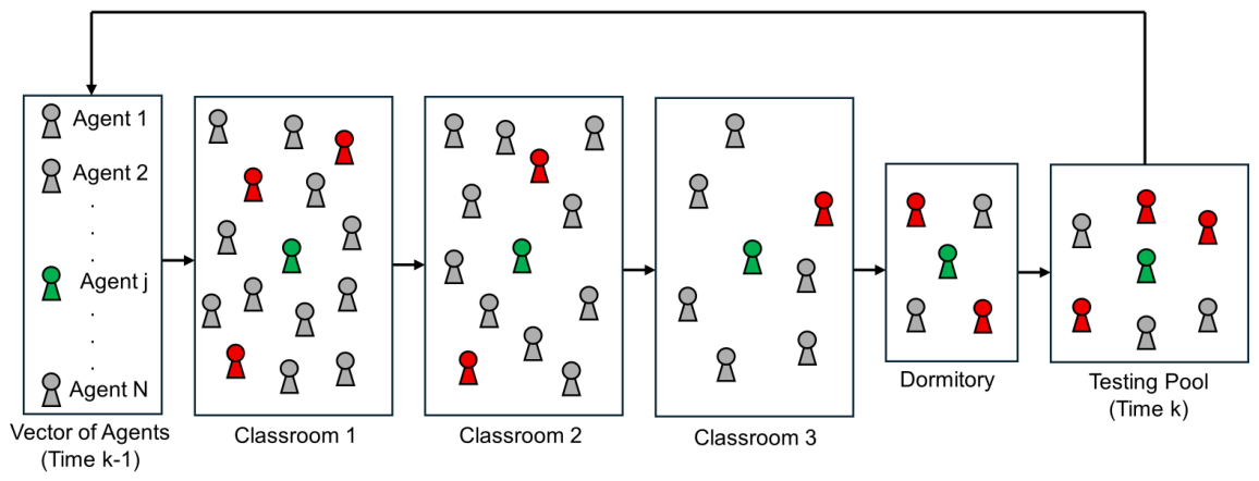
Agents move according to a location schedule ${\mathcal{L}}_k=\{L_1\left(k\right),L_2\left(k\right),\dots ,L_N\left(k\right)\}$, where $L_i\left(k\right)\subseteq \{1,\dots ,M\}$ denotes the subset of M locations agent i visits at time k. At each location j, agents interact according to a contact schedule ${\mathcal{C}}_{jk}=\{C_1(j,k),C_2(j,k),\dots ,C_N(j,k)\}$, where $C_i(j,k)\subseteq \{1,\dots ,N\}$ denotes the set of agents that agent i contacts at location j at time k. Let ${\mathcal{C}}_k=\{C_{1k},\dots ,C_{Mk}\}$ denote the set of all scheduled contacts at time k. These contacts might represent household interactions (daily, fixed contacts), workplace interactions (weekday patterns), social interactions (varying contacts), or community interactions (spatial proximity). Figure 1 depicts a typical contact structure and observation for an agent on a university campus.

Susceptible to Exposed Transition: For a susceptible agent i, denote:

$$p_{ij}=1-\prod _{l\in C_i(j,k)}(1-{\lambda }_E·{\mathbb{I}}_I(l,k-1))$$

(3)

where ${\lambda }_E\in [0,1]$ is the per-contact transmission probability and ${\mathbb{I}}_I(l,k-1)$ is an indicator function equal to 1 if agent l is in the infected state at time $k-1$. This captures independent exposure chances for all contacts in $C_i(j,k)$. The probability of transitioning to exposed at time k is:

$$P(S_i\to E_i\mid {\mathbf{X}}_{k-1},{\mathcal{L}}_k,{\mathcal{C}}_k)=1-(1-\theta )·\prod _{j\in L_i\left(k\right)}(1-e_j·p_{ij})$$

(4)

where $\theta \in [0,1]$ is the spontaneous exposure rate, and $e_j\in [0,1]$ is an environmental risk factor associated with location j. This captures independent exposure chances across all locations in $L_i\left(k\right)$. For brevity, we suppress the dependencies and use $P(S_i\to E_i)$ going forward.

Exposed to Infected Transition: Exposed agents transition to infected with probability ${\lambda }_I$ per time step:

$$P(E_i\to I_i)={\lambda }_I$$

(5)

where $1/{\lambda }_I$ represents the mean incubation period.

Infected to Recovered Transition: Infected agents recover with probability ${\lambda }_R$ per time step:

$$P(I_i\to R_i)={\lambda }_R$$

(6)

where $1/{\lambda }_R$ represents the mean infectious period.

3.2.2. Observation Model

Let $y_i^j\in \mathbb{B}$ denote the observation of bit j belonging to a tested agent $i\in {\mathcal{T}}_k$. Then for each agent $i\in {\mathcal{T}}_k$, the observation model independently measures each bit as a Bernoulli trial with errors

$$\begin{array}{c}\hfill P(y_i^1=1\mid b_i^1=0)=\alpha \\ \hfill P(y_i^1=0\mid b_i^1=1)=\beta \\ \hfill P(y_i^2=1\mid b_i^2=0)=\gamma \\ \hfill P(y_i^2=0\mid b_i^2=1)=\delta \end{array}$$

(7)

3.3. Inference Approaches

The central challenge of epidemic state estimation is computing the posterior distribution $p\left({\mathbf{X}}_k\right|{\mathbf{Y}}_{1:k})$ over all agent states given all observations up to time k. We develop two complementary approaches tailored to different population scales.

3.3.1. Boolean Kalman Particle Filter

For populations where $N\lesssim 100$, we maintain a set of $N_p$ particles ${\left\{{\mathbf{x}}_{k,m}\right\}}_{m=1}^{N_p}$, where each particle ${\mathbf{x}}_{k,m}$ is a complete hypothesis about all N agents’ Boolean states. The particle filter approximates the posterior distribution as follows:

$$p\left({\mathbf{X}}_k\right|{\mathbf{Y}}_{1:k})\approx {\displaystyle \sum _{m=1}^{N_p}}{W}_{k,m}\delta ({\mathbf{X}}_k-{\mathbf{x}}_{k,m})$$

(8)

where $W_{k,m}$ are importance weights and $\delta (·)$ is the Dirac delta function assigning point mass probability to each particle ${\mathbf{x}}_{k,m}$.

The agent-based SEIR dynamics define a state transition distribution $p\left({\mathbf{X}}_k\right|{\mathbf{X}}_{k-1})$ through the stochastic function $f_k({\mathbf{X}}_{k-1},{\mathbf{n}}_k)$ described by Equations (3)–(6). These equations define per-agent transition probabilities that are independent Bernoulli trials given the previous state ${\mathbf{X}}_{k-1}$. This conditional independence allows the state transitions to factorize:

$$p\left({\mathbf{X}}_k\right|{\mathbf{X}}_{k-1})={\displaystyle \prod _{i=1}^N}p\left(X_k^{\left(i\right)}\right|{\mathbf{X}}_{k-1}).$$

(9)

Two important distributions are the look-ahead distribution, $p({\mathbf{Y}}_k\mid {\mathbf{X}}_{k-1})$, and the guided proposal distribution, $p({\mathbf{X}}_k\mid {\mathbf{X}}_{k-1},{\mathbf{Y}}_k)$. If observations are conditionally independent, the look-ahead becomes the following:

$$p({\mathbf{Y}}_k\mid {\mathbf{X}}_{k-1})={\displaystyle \prod _{i=1}^N}\sum _{X_k^{\left(i\right)}\in {\{0,1\}}^2}p(Y_k^{\left(i\right)}\mid X_k^{\left(i\right)})p(X_k^{\left(i\right)}\mid {\mathbf{X}}_{k-1})$$

(10)

where $p(Y_k^{\left(i\right)}\mid X_k^{\left(i\right)})=1$ for $i\notin {\mathcal{T}}_k$ (untested agents). The guided proposal $p({\mathbf{X}}_k\mid {\mathbf{X}}_{k-1},{\mathbf{Y}}_k)=p({\mathbf{Y}}_k\mid {\mathbf{X}}_k)p({\mathbf{X}}_k\mid {\mathbf{X}}_{k-1})/p({\mathbf{Y}}_k\mid {\mathbf{X}}_{k-1})$ factorizes identically:

$$p({\mathbf{X}}_k\mid {\mathbf{X}}_{k-1},{\mathbf{Y}}_k)={\displaystyle \prod _{i=1}^N}{\displaystyle \frac{p(Y_k^{\left(i\right)}\mid X_k^{\left(i\right)})p(X_k^{\left(i\right)}\mid {\mathbf{X}}_{k-1})}{{\sum }_{X_k^{\left(i\right)}\in {\{0,1\}}^2}p(Y_k^{\left(i\right)}\mid X_k^{\left(i\right)})p(X_k^{\left(i\right)}\mid {\mathbf{X}}_{k-1})}}$$

(11)

We now reproduce the APF-BKF of Imani and Braga-Neto [3] adapted to our epidemiological model. Given particles ${\left\{{\mathbf{x}}_{k,m}\right\}}_{m=1}^{N_p}$ and initial distribution $p\left({\mathbf{X}}_0\right)$, sample ${\mathbf{X}}_{0,m}\sim p\left({\mathbf{X}}_0\right)$, and initialize weights $W_{0,m}=1/N_p$, for $m=1,\dots ,N_p$. For each time step $k=1,2,\dots$:

• Compute first-stage weights: $V_{k,m}=p({\mathbf{Y}}_k\mid {\mathbf{x}}_{k-1,m})W_{k-1,m}$ for $m=1,\dots ,N_p$.
• Sample auxiliary variables: ${\left\{{\zeta }_{k,m}\right\}}_{m=1}^{N_p}\sim \mathrm{Cat}\left({\left\{V_{k,m}\right\}}_{m=1}^{N_p}\right)$.
• Obtain new particles from the guided proposal: ${\mathbf{x}}_{k,m}\sim p({\mathbf{X}}_k\mid {\mathbf{x}}_{k-1,{\zeta }_{k,m}},{\mathbf{Y}}_k)$.
• Compute second-stage weights:

  $${\tilde{W}}_{k,m}={\displaystyle \frac{p({\mathbf{Y}}_k\mid {\mathbf{x}}_{k,m})p({\mathbf{x}}_{k,m}\mid {\mathbf{x}}_{k-1,{\zeta }_{k,m}})}{p({\mathbf{x}}_{k,m}\mid {\mathbf{x}}_{k-1,{\zeta }_{k,m}},{\mathbf{Y}}_k)}}$$

  (12)
• Normalize: $W_{k,m}={\tilde{W}}_{k,m}/{\sum }_{j=1}^{N_p}{\tilde{W}}_{k,j}$.
• Compute expectation: ${\mathbf{z}}_k={\sum }_{m=1}^{N_p}{W}_{k,m}{\mathbf{x}}_{k,m}$.
• Compute minimum mean square error (MMSE) estimate: ${\widehat{\mathbf{X}}}_k^{\mathrm{MS}}={\overline{\mathbf{z}}}_k$ where ${\overline{\mathbf{z}}}_k(i,j)=1$ if ${\mathbf{z}}_k(i,j)>1/2$, else 0 (elementwise thresholding at 1/2).
• Compute mean square error (MSE): $\mathrm{MSE}({\widehat{\mathbf{X}}}_k^{\mathrm{MS}},{\mathbf{Y}}_{1:k})={\parallel \min \{{\mathbf{z}}_k,{\mathbf{z}}_k^c\}\parallel }_1$ where ${\mathbf{z}}_k^c(i,j)=1-{\mathbf{z}}_k(i,j)$, min is performed elementwise, and ${\parallel ·\parallel }_1$ denotes the matrix $L_1$ norm.

Note that while the MSE in step 8 may not look like a conventional expectation of an $L_2$ norm, it is indeed the true MSE in the space of binary vectors. Also note, if the exact look-ahead and guided proposal are used (conditional independence holds), then the second stage weights are uniform.

$$\begin{array}{cc}\hfill {\displaystyle \frac{p({\mathbf{Y}}_k\mid {\mathbf{x}}_{k,m})p({\mathbf{x}}_{k,m}\mid {\mathbf{x}}_{k-1,{\zeta }_{k,m}})}{p({\mathbf{x}}_{k,m}\mid {\mathbf{x}}_{k-1,{\zeta }_{k,m}},{\mathbf{Y}}_k)}}& ={\displaystyle \frac{p({\mathbf{Y}}_k\mid {\mathbf{x}}_{k,m})p({\mathbf{x}}_{k,m}\mid {\mathbf{x}}_{k-1,{\zeta }_{k,m}})}{p({\mathbf{Y}}_k\mid {\mathbf{x}}_{k,m})p({\mathbf{x}}_{k,m}\mid {\mathbf{x}}_{k-1,{\zeta }_{k,m}})/p({\mathbf{Y}}_k\mid {\mathbf{x}}_{k-1,{\zeta }_{k,m}})}}\hfill \\ \hfill & =p({\mathbf{Y}}_k\mid {\mathbf{x}}_{k-1,{\zeta }_{k,m}})\hfill \end{array}$$

(13)

Since the first stage weights use the look-ahead $p({\mathbf{Y}}_k\mid {\mathbf{x}}_{k-1,m})W_{k-1,m}$ to sample ${\zeta }_{k,m}$, then the final weights become uniform under the fully adapted proposal.

3.3.2. Mean-Field Approximation for Large Populations

For populations where $N\gtrsim 100$, the state space of $4^N$ configurations becomes intractable. We employ a mean-field (MF) approximation that factorizes the posterior:

$$p\left({\mathbf{X}}_k\right|{\mathbf{Y}}_{1:k})\approx {\displaystyle \prod _{i=1}^N}{q}_k^{\left(i\right)}\left(X_k^{\left(i\right)}\right)$$

(14)

where $q_k^{\left(i\right)}\left(s\right)=p(X_k^{\left(i\right)}=s\mid {\mathbf{Y}}_{1:k})$ for $s\in \{S,E,I,R\}$ is the marginal distribution for agent i. Each marginal is represented as a probability vector of length 4:

$${\mathbf{q}}_k^{\left(i\right)}={[q_k^{\left(i\right)}\left(S\right),q_k^{\left(i\right)}\left(E\right),q_k^{\left(i\right)}\left(I\right),q_k^{\left(i\right)}\left(R\right)]}^{\top }.$$

(15)

This requires storing only $4N$ probability values rather than tracking $4^N$ joint configurations.

Mean-Field Prediction Step: At time k, we compute the expected infection pressure each agent faces. For agent i at location j, we use a moment closure in place of Equation (3) for the mean-field infection probability:

$${\overline{p}}_{ij}=1-\prod _{l\in C_i(j,k)}\left(1-\eta ·{\lambda }_E·q_{k-1}^{\left(l\right)}\left(I\right)\right)$$

(16)

where $\eta \in [0,1]$ is an effective infectious susceptibility scaling parameter that accounts for over-mixing in the mean field approximation, and $q_{k-1}^{\left(l\right)}\left(I\right)$ is the probability that agent l is infected at time $k-1$.

The predicted marginal distribution for agent i at time k is the following:

$$\begin{array}{cc}\hfill q_k^{\left(i\right)-}\left(S\right)& =q_{k-1}^{\left(i\right)}\left(S\right)·\left(1-P(S_i\to E_i)\right)\hfill \\ \hfill q_k^{\left(i\right)-}\left(E\right)& =q_{k-1}^{\left(i\right)}\left(S\right)·P(S_i\to E_i)+q_{k-1}^{\left(i\right)}\left(E\right)·(1-{\lambda }_I)\hfill \\ \hfill q_k^{\left(i\right)-}\left(I\right)& =q_{k-1}^{\left(i\right)}\left(E\right)·{\lambda }_I+q_{k-1}^{\left(i\right)}\left(I\right)·(1-{\lambda }_R)\hfill \\ \hfill q_k^{\left(i\right)-}\left(R\right)& =q_{k-1}^{\left(i\right)}\left(I\right)·{\lambda }_R+q_{k-1}^{\left(i\right)}\left(R\right)\hfill \end{array}$$

(17)

where the superscript $(-)$ denotes the predicted distribution before incorporating observations.

Mean-Field Update Step: When agent i is observed at time k with measurement $Y_k^{\left(i\right)}$, we update only that agent’s marginal using Bayes’ rule:

$$q_k^{\left(i\right)}\left(s\right)={\displaystyle \frac{p\left(Y_k^{\left(i\right)}\right|X_k^{\left(i\right)}=s)·q_k^{\left(i\right)-}\left(s\right)}{{\sum }_{s^{\prime }\in \{S,E,I,R\}}p\left(Y_k^{\left(i\right)}\right|X_k^{\left(i\right)}=s^{\prime })·q_k^{\left(i\right)-}\left(s^{\prime }\right)}}$$

(18)

Note that this differs from updating the full joint distribution, where a positive test for one agent can provide information on other agents through the contact network. For agents not observed at time k, the marginal remains unchanged: $q_k^{\left(i\right)}\left(s\right)=q_k^{\left(i\right)-}\left(s\right)$. These marginals are then converted to the Boolean state vector according to our two-bit encoding:

$$z_k^{\left(i\right)}=[q_k^{\left(i\right)}\left(E\right)+q_k^{\left(i\right)}\left(I\right),q_k^{\left(i\right)}\left(I\right)+q_k^{\left(i\right)}\left(R\right)],i=1,\dots ,N$$

(19)

with MMSE state estimate and MSE computed following the APF-BKF algorithm. Note that the MSE may no longer be optimal as we are no longer targeting the joint distribution.

4. Results

We evaluate our BS-ABM frameworks on two realistic campus scenarios demonstrating different inference methodologies necessitated by computational constraints:

• Small College (100 agents): We apply the Boolean Kalman particle filter (BKF) with $4\times {10}^6$ particles.
• Large University (50,000 agents): We employ mean-field approximation with linear computational complexity.

Both scenarios assess the ability to reconstruct population-level infection dynamics and individual agent states from sparse, noisy testing data.

Agent schedules are generated as follows. During weekdays, both campuses operate on five class periods per day. Each agent attends three of the five periods in randomly selected classrooms, yielding 15 class meetings per week. No classes occur on weekends. This weekly schedule repeats over 100 days. Additionally, a specified fraction of agents live in dormitories, interacting with roommates daily (including weekends).

For each campus, we run simulations for two outbreak regimes. In the small outbreak regime, classroom and dormitory environmental risk factors are sampled uniformly in [0.1, 0.2], and ${\lambda }_E=0.01$. In the large outbreak regime, risk factors are sampled from [0.2, 0.3], and ${\lambda }_E=0.05$. For all experiments, ${\lambda }_I=1/5$ and ${\lambda }_R=1/10$.

For all combinations of campus size, outbreak regime, and testing strategy, an ensemble of 100 randomly initialized schedules, environmental risk factors, and five initially infected agents were sampled. All parameters are summarized in

Table A1. Model Parameters.

Parameter	Small College	Large University	Description
${\lambda }_E$ (small outbreak)	0.01	0.01	Probability of S → E
${\lambda }_E$ (large outbreak)	0.05	0.05	Probability of S → E
${\lambda }_I$	1/5	1/5	Probability of E → I
${\lambda }_R$	1/10	1/10	Probability of I → R
off_campus	0.5	0.8	Portion of agents living off campus
off_exp	${10}^{-3}$	${10}^{-6}$	Off campus probability of S → E
$c_j$ (small outbreak)	Unif ([0.1, 0.2])	Unif ([0.1, 0.2])	Classroom risk factors
$c_j$ (large outbreak)	Unif ([0.2, 0.3])	Unif ([0.2, 0.3])	Classroom risk factors
$d_j$ (small outbreak)	Unif ([0.1, 0.2])	Unif ([0.1, 0.2])	Dormitory risk factors
$d_j$ (large outbreak)	Unif ([0.2, 0.3])	Unif ([0.2, 0.3])	Dormitory risk factors
$\theta$	${10}^{-4}$	${10}^{-6}$	Spontaneous exposure rate
$\alpha$	0.05	0.05	First bit false positive rate
$\beta$	0.05	0.05	First bit false negative rate
$\gamma$	0.05	0.05	Second bit false positive rate
$\delta$	0.05	0.05	Second bit false negative rate
$\eta$	N/A	0.9	Infectious susceptibility scaling factor
$N_p$	$4\times {10}^6$	N/A	Number of particles

.

All experiments were originally run as Google Colab notebooks in an L4 GPU environment with 24 GB of RAM and took approximately 15 h of wall time with a single BKF simulation day taking approximately 810 ms, and a single MF simulation day taking approximately 90 ms. The source code used to generate our results can be found at https://github.com/UBragaNeto/State-Space_Agent-Based_Model_Infectious_Disease, accessed on 6 May 2026.

4.1. Observation Model Parameters

At each time step, we independently test $N_T$ agents selected randomly. Each test measures both Boolean state bits with symmetric error rates: false positive rate $\alpha =0.05$ and false negative rate $\beta =0.05$ for the first bit, and false positive rate $\gamma =0.05$ and false negative rate $\delta =0.05$ for the second bit. We evaluate testing rates of 1%, 5%, and 10% of the population per day.

4.2. Quantities of Interest

We analyze several performance metrics:

Ground Truth Test Error: The portion of tested agents whose tests do not match their true state. With symmetric 5% error on both bits, expected error is $P\left(\mathrm{state}\mathrm{error}\right)=1-$$P\left(\mathrm{bit}1\mathrm{correct}\right)P\left(\mathrm{bit}2\mathrm{correct}\right)=1-{0.95}^2=0.0975$.

BKF/MF Test Error: The portion of tested agents whose BKF/MF states do not match their true states. Our model incorporates test error information via the likelihood, so we expect agents in the test set to be closer to ground truth in the BKF/MF than their naïve test results would indicate.

BKF/MF Total Error: The portion of all agents whose BKF/MF states do not match their true states. This evaluates the quality of estimates for untested agents.

BKF/MF Precision: Measures the accuracy of positive predictions (exposed or infected) as the ratio of true positives over true positives + false positives.

BKF/MF Recall: Measures the ability to find all positives (exposed or infected) as the ratio of true positives over true positives + false negatives.

Relative $L_1$ Error of E + I Counts: Let $\widehat{E}={[{\widehat{E}}_1,\dots ,{\widehat{E}}_{100}]}^{\top }$ denote the vector of Exposed agents predicted by the BKF/MF over 100 days, and let $\tilde{E}$ denote ground truth. Similarly, define $\widehat{I}$ and $\tilde{I}$ for Infectious agents. The relative $L_1$ error on E + I counts is $\parallel (\widehat{E}+\widehat{I})-(\tilde{E}+\tilde{I}){\parallel }_1/{\parallel \tilde{E}+\tilde{I}\parallel }_1$.

Ground Truth Within MSE: To determine uncertainty quantification calibration, we measure the portion of ground truth E + I counts that lie in the interval $\tilde{E}+\tilde{I}\in [\widehat{E}+\widehat{I}-\mathrm{MSE},$$\widehat{E}+\widehat{I}+\mathrm{MSE}]$.

4.3. Small College Environment: Particle Filter Approach

The small college comprises 100 agents moving among three classroom buildings and three dormitories over 100 days. Half the population lives on campus; the other half lives off campus with a daily exposure probability of ${10}^{-3}$. The spontaneous exposure rate $\theta$ is ${10}^{-4}$.

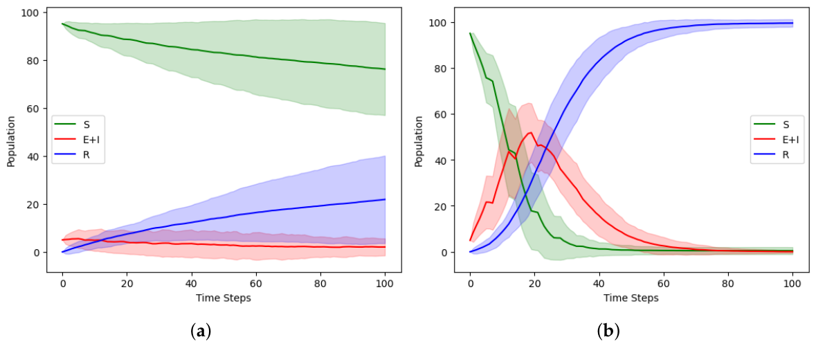
The small outbreak regime had an average size of 3.12 infections with a peak of 7.68. The large outbreak regime had an average size of 14.61 infections with a peak of 54.23. Figure 2a,b show 100 random initialization mean and $\pm 2$ standard deviation Susceptible (S), Exposed + Infected (E + I), and Recovered (R) curves for the small outbreak and large outbreak regimes, respectively.

Small Outbreak Performance:

Table 1. Small College, Small Outbreak Boolean Kalman Particle Filter (BKF) Results.

Test Rate (%)	1	5	10
Ground Truth Test Error	0.0998	0.0936	0.0968
BKF Test Error	0.0588	0.0553	0.0460
BKF Total Error	0.1411	0.1014	0.0747
BKF Precision	0.6703	0.6688	0.6995
BKF Recall	0.0261	0.1343	0.2680
BKF E + I Relative $L_1$ Error	0.6942	0.5630	0.5104
Ground Truth Within MSE	0.9994	0.9803	0.9394

summarizes results averaged over 100 ensembles. At a 1% test rate, BKF test error is roughly half the ground truth test error (0.0588 vs. 0.0998). This improves to less than half at 10% testing (0.0460 vs. 0.0968), indicating growing ability to outperform naïve test results as observations increase.

The total BKF error begins at 0.1411, showing an accurate prediction of 85.89% of agent states with noisy data on only 1% of the population. This improves to 92.53% accuracy at 10% testing. Precision begins at 0.6703 and slightly increases to 0.6995, indicating nearly 70% accuracy in reported exposed and infected states for all test rates. Recall starts quite low at 0.0261, but is over double the testing rate of 1%. It remains over double the testing rate as it climbs to 10%, indicating an ability to find exposed and infected agents at a higher rate than naïve testing.

At 1% testing, relative $L_1$ error is 0.6942 (approximately $\pm 2$ E + I counts around the 3.12 average) with 99.94% of error captured within MSE. At 10% testing, error drops to 0.5104 ($\pm 1.5$ counts) with 93.94% MSE coverage, indicating the BKF becomes slightly overconfident as observations become more informative.

Large Outbreak Performance:

Table 2. Small College, Large Outbreak BKF Results.

Test Rate (%)	1	5	10
Ground Truth Test Error	0.0968	0.0939	0.0950
BKF Test Error	0.0478	0.0457	0.0483
BKF Total Error	0.1750	0.1612	0.1445
BKF Precision	0.5654	0.6056	0.6591
BKF Recall	0.2195	0.4521	0.5599
BKF E + I Relative $L_1$ Error	0.1575	0.1490	0.1459
Ground Truth Within MSE	0.9003	0.8880	0.8667

summarizes results. For all testing rates, BKF test error remains around half the ground truth error, indicating the BKF outperforms naïve tests even as SEIR states become broadly distributed.

BKF total error begins at 0.1750 (82.50% accuracy with a single daily test) and improves to 85.55% at 10% testing, showing modest improvement with tenfold increase in observations. Precision begins at 0.5654 at a 1% test rate and climbs to 0.6591 at 10% testing. This is lower than the small outbreak scenario since agent states are more scattered, making them less reliable to predict, but there is a noticeable increase in performance with the testing rate that the small outbreak scenario lacks. Recall starts much higher than the small outbreak at 0.2195 and similarly grows with the test rate, indicating a better ability to find exposed and infected agents when the outbreak signal is large.

Relative $L_1$ error begins at 0.1575 ($\pm 2.3$ counts around the 14.61 average) with 90.03% error within MSE. This demonstrates strong ability to track large outbreaks with a single daily test. Error improves modestly with increased testing, again becoming slightly overconfident.

4.4. Large University Environment: Mean-Field Approach

The large university comprises 50,000 agents moving among 1000 classrooms and 5000 dormitories over 100 days. 20% live on campus; the other 80% have daily exposure probability of ${10}^{-6}$. The spontaneous exposure rate $\theta$ is ${10}^{-6}$, and effective infectious susceptibility scaling $\eta$ is 0.9. This choice of $\eta =0.9$ was found to best fit the simulation data and does not seem overly sensitive to deviations, with $\eta \in [0.8,1.0]$ yielding similar results.

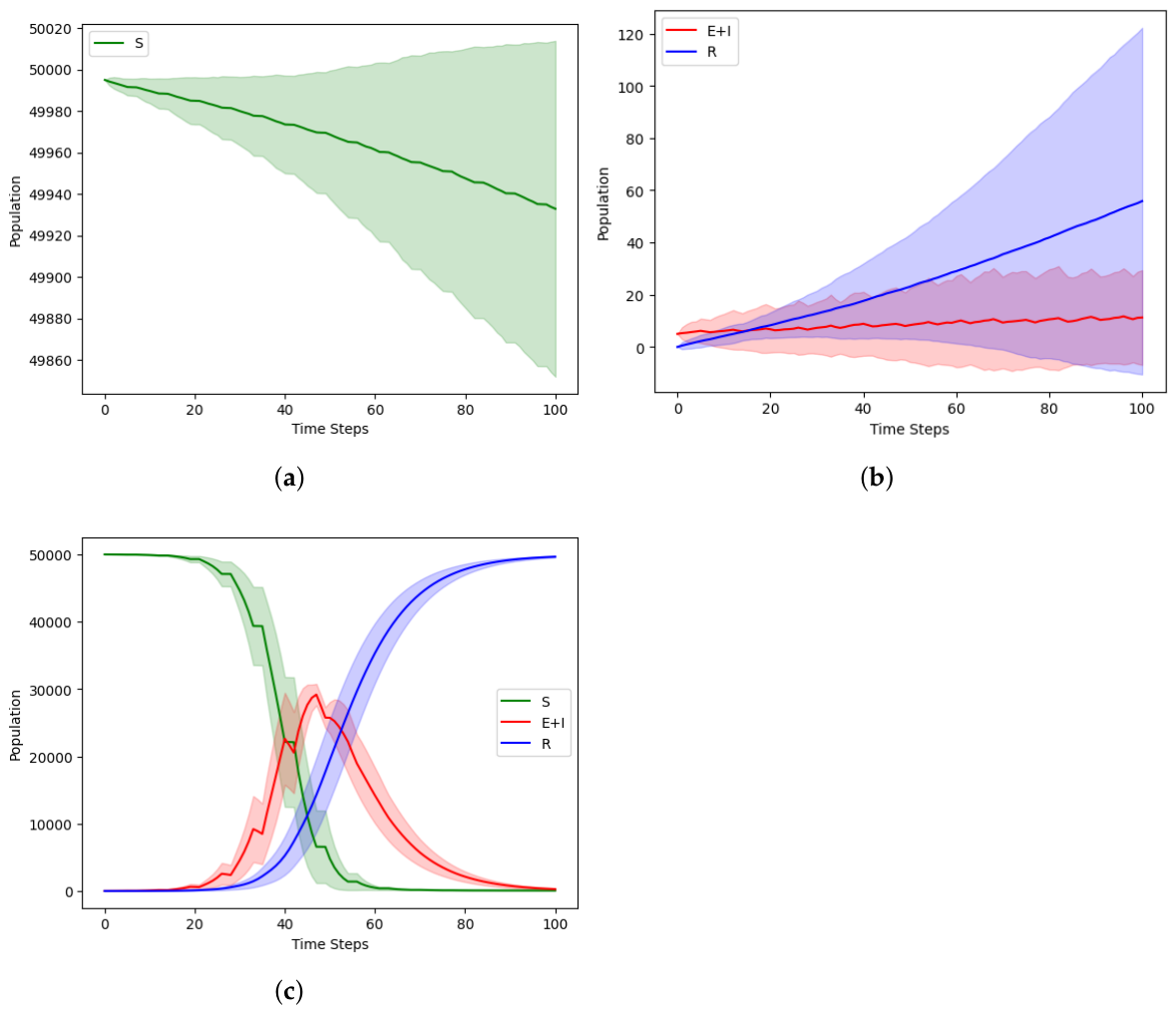
The small outbreak regime had an average size of 8.57 infections with a peak of 17.13. The large outbreak regime had average size 7393 infections with peak 29,329. Figure 3a–c show 100 random initialization mean and ±2 standard deviation S, E + I, and R curves for the small outbreak S, small outbreak E + I and R, and large outbreak regimes, respectively.

Small Outbreak Performance:

Table 3. Large University, Small Outbreak Mean-Field (MF) Results.

Test Rate (%)	1	5	10
Ground Truth Test Error	0.0974	0.0975	0.0974
MF Test Error	0.0007	0.0004	0.0003
MF Total Error	0.0007	0.0005	0.0004
MF Precision	0.6859	0.7025	0.7258
MF Recall	0.0015	0.0352	0.1282
MF E + I Relative $L_1$ Error	0.7391	0.6258	0.4922
Ground Truth Within MSE	0.9929	0.9986	0.9974

summarizes results. MF test error performs much better than the expected ground truth error of 0.0975. At 1% testing, MF achieves test error 0.0007, improving to 0.0003 at 10%. Total error ranges from 0.0007 at 1% to 0.0004 at 10%. While seemingly exceptional, these results reflect that >99% of the population remain susceptible, with errors occurring predominantly around the average 8.57 E + I agents out of 50,000.

Precision at a 1% testing rate is 0.6859, rising to 0.7258 at 10% testing. This similarly hovers around the 70% value of the small college, small outbreak scenario, but now with a larger improvement as the test rate grows. Recall is woefully below the 1% test rate at 0.0015; however, it grows above the 10% test rate at 0.1282. This indicates the mean field approximation needs more tests to start capturing the exposed and infected agents for small outbreaks.

Relative $L_1$ error starts at 0.7391 at 1% testing (approximately ±6 E + I counts around the 8.57 average) with 99.29% error within MSE. At 10% testing, error drops to 0.4922 (±4 counts) with 99.74% MSE coverage. All testing rates show the MF’s ability to capture the endemic nature with very few estimates dying off or blowing up.

Large Outbreak Performance:

Table 4. Large University, Large Outbreak MF Results.

Test Rate (%)	1	5	10
Ground Truth Test Error	0.0972	0.0974	0.0974
MF Test Error	0.0447	0.0368	0.0313
MF Total Error	0.1657	0.1425	0.1211
MF Precision	0.5715	0.6534	0.7097
MF Recall	0.3505	0.5090	0.6298
MF E + I Relative $L_1$ Error	0.0931	0.0431	0.0221
Ground Truth Within MSE	0.9999	0.9999	0.9998

summarizes results. MF test error begins at half the ground truth at 1% testing (0.0447 vs. 0.0972) and drops to a third at 10% (0.0313 vs. 0.0974). Unlike the small outbreak, where nearly everyone remains susceptible, the large outbreak can have the population in any mixture of SEIR states. The MF demonstrates clear ability to outperform naïve test results.

Total error begins at 0.1657 at 1% testing, indicating accurate prediction of 83.43% of states with noisy tests on only 1% in any SEIR configuration. Performance increases to 87.89% accuracy at 10% testing. Precision starts similar to the small college, large outbreak scenario at 0.5715 for 1% testing. It then increases at a slightly faster rate to 0.7097 at 10% testing. Recall is much improved for large outbreaks, starting at 0.3505 for 1% testing and growing to 0.6298 at 10%, showing a strong ability to find exposed and infected agents far above the testing rate.

Relative $L_1$ error begins at 0.0931 (roughly ±688 E + I counts around the 7393 average) and drops to 0.0221 at 10% testing (±163 counts). This is exceptional performance with nearly all errors (0.9998–0.9999) captured within MSE, indicating nearly perfect uncertainty quantification for all test rates.

4.5. Key Findings

Results demonstrate several important insights:

Scaling Transition: Experiments illustrate a practical transition from exact particle filtering (small college, $N=100$) to scalable mean-field inference (large university, N = 50,000). The mean-field approximation scales linearly with population size and remains effective at realistic scales.

Statistical Denoising: Both methods provide clear evidence of denoising relative to raw test outcomes. With 5% bit error, naïve tests show ∼9.75% error. In small college experiments, BKF reduces tested-agent error by approximately half in both outbreak regimes. In large university experiments, mean-field similarly improves substantially over naïve tests in large outbreaks; in small outbreaks, extremely low error reflects that nearly all agents remain susceptible.

Outbreak Magnitude Effects: Outbreak magnitude strongly affects difficulty. In both environments, large outbreaks are easier to track in aggregate epidemic intensity. For the small college, large outbreaks yield low relative errors (0.1459–0.1575), whereas small outbreaks are more difficult (0.5104–0.6942). The pattern amplifies in the large university: small outbreaks have large relative errors (0.4922–0.7391), while large outbreaks are tracked closely (0.0221–0.0931). Similar findings occur for recall. Small college, large outbreaks have substantially larger recall (0.2195–0.5599) compared with small outbreaks (0.0261–0.2680). The large university is similar, where large outbreak recall (0.3505–0.6298) drastically outperforms small outbreaks (0.0015–0.1282). When few agents are infected, the epidemic signal is weak; when many are infected, the system provides a stronger aggregate signal.

Testing Rate Diminishing Returns: Increasing testing from 1% to 5% produces noticeable improvement. Additional improvement from 5% to 10% is smaller, suggesting that modest daily testing provides the most benefit for population-level monitoring.

Uncertainty Calibration: Small college, small outbreaks show near-perfect coverage at low test rates (0.9994 at 1%) but decrease as tests become more informative (0.9394 at 10%), indicating mild overconfidence. In small colleges, large outbreaks, coverage is lower overall (0.8667–0.9003). By contrast, in large university, large outbreaks, MF coverage is essentially perfect (0.9998–0.9999). All experiments maintained >86% coverage, showing strong uncertainty calibration.

Particle Filter vs. Mean-Field Tradeoff: Particle filtering provides principled approximation of the full joint posterior, with strong performance for small populations under sparse testing, but computational cost limits use at large N. Mean-field sacrifices joint correlation structure, but offers linear-time scalability and, in these regimes, delivers accurate reconstruction of both individual states and population-level epidemic intensity.

5. Conclusions

We have presented a comprehensive framework for epidemic state estimation that combines Boolean state-space representations of agent-based SEIR models with optimal filtering methods tailored to different population scales. Our key contributions include the following: (1) formal Boolean encoding of epidemiological states enabling discrete-state optimal filtering; (2) application of Boolean Kalman particle filtering to small populations demonstrating accurate inference from sparse, noisy observations; (3) development of mean-field approximation for large populations achieving linear computational complexity while maintaining accuracy and (4) comprehensive empirical evaluation across multiple outbreak scenarios, testing rates, and population scales.

Our experimental results demonstrate that mean-field approximations achieve exceptional performance when populations are large and epidemic signals are strong, even 1% daily testing rates enable accurate population-level monitoring, and large outbreaks are easier to track due to a high signal-to-noise ratio. The Boolean state-space framework, combined with scale-appropriate inference methods, provides a promising foundation for real-time epidemic monitoring systems balancing modeling fidelity, computational efficiency, and estimation accuracy.

Future Directions

Several promising extensions warrant future investigation:

Hybrid Particle Filter / Mean-Field Methods: Our results suggest that particle filtering excels at capturing correlations in small groups while mean-field scales to large populations. A hybrid approach that applies particle filtering to highly connected subpopulations (e.g., households, classrooms) while using mean-field for inter-group interactions could combine the strengths of both methods.

Adaptive Testing Strategies: While we used fixed-rate random testing, a more sophisticated strategy based on the selection of agents with maximal MSE could further reduce testing requirements. This would alter the observation model to account for probabilistic selection of the test set and may break the conditional independence assumption in the likelihood.

Parameter Learning: Our current framework assumes known parameters (Test Rate, ${\lambda }_E$, ${\lambda }_I$, ${\lambda }_R$, $c_j$, $d_j$, $\alpha$, $\beta$, $\gamma$, $\delta$, $\eta$, $\theta$). Joint state and parameter estimation using particle MCMC or variational methods could enable real-time parameter learning from surveillance data [3].

Extended States: Extending the Boolean representation to handle symptomatic status, vaccination status, or multiple circulating strains (requiring additional Boolean bits per agent) would enable modeling of competitive dynamics and strain-specific interventions.

References

1. Ferguson, N.M.; Laydon, D.; Nedjati-Gilani, G.; Imai, N.; Ainslie, K.; Baguelin, M.; Bhatia, S.; Boonyasiri, A.; Cucunubá, Z.; Cuomo-Dannenburg, G.; et al. Report 9: Impact of Non-Pharmaceutical Interventions (NPIs) to Reduce COVID-19 Mortality and Healthcare Demand; Imperial College London: London, UK, 2020. [Google Scholar] [CrossRef]
2. Keeling, M.J.; Rohani, P. Modeling Infectious Diseases in Humans and Animals, 1st ed.; Princeton University Press: Princeton, NJ, USA, 2011; pp. 15–104. [Google Scholar] [CrossRef]
3. Imani, M.; Braga-Neto, U.M. Particle filters for partially-observed Boolean dynamical systems. Automatica 2018, 87, 238–250. [Google Scholar] [CrossRef]
4. Doucet, A.; De Freitas, N.; Gordon, N. Sequential Monte Carlo Methods in Practice, 1st ed.; Springer: New York, NY, USA, 2001; pp. 17–41. [Google Scholar] [CrossRef]
5. Snyder, C.; Bengtsson, T.; Bickel, P.; Anderson, J. Obstacles to high-dimensional particle filtering. Mon. Weather Rev. 2008, 136, 4629–4640. [Google Scholar] [CrossRef]
6. Wainwright, M.J.; Jordan, M.I. Graphical models, exponential families, and variational inference. Found. Trends Mach. Learn. 2008, 1, 1–305. [Google Scholar] [CrossRef]
7. Kermack, W.O.; McKendrick, A.G. A contribution to the mathematical theory of epidemics. Proc. R. Soc. Lond. Proc. A 1927, 115, 700–721. [Google Scholar] [CrossRef]
8. Tracy, M.; Cerdá, M.; Keyes, K.M. Agent-Based Modeling in Public Health: Current Applications and Future Directions. Annu. Rev. Public Health 2018, 39, 77–94. [Google Scholar] [CrossRef] [PubMed]
9. Zhang, X.; Wang, J.; Yu, C.; Fei, J.; Luo, T.; Cao, Z. Agent-Based Modeling of Epidemics: Approaches, Applications, and Future Directions. Technologies 2025, 13, 272. [Google Scholar] [CrossRef]
10. Kraul, M.; Zimmerman, R.K.; Williams, K.V.; Raviotta, J.M.; Harrison, L.H.; Williams, J.V.; Roberts, M.S. Agent-based model of the impact of higher influenza vaccine efficacy on seasonal influenza burden. Vaccine X 2023, 13, 100249. [Google Scholar] [CrossRef]
11. Kerr, C.C.; Stuart, R.M.; Mistry, D.; Abeysuriya, R.G.; Rosenfeld, K.; Hart, G.R.; Núñez, R.C.; Cohen, J.A.; Selvaraj, P.; Hagedorn, B.; et al. Covasim: An agent-based model of COVID-19 dynamics and interventions. PLoS Comput. Biol. 2021, 17, e1009149. [Google Scholar] [CrossRef] [PubMed]
12. Kalman, R.E. A new approach to linear filtering and prediction problems. J. Basic Eng. 1960, 82, 35–45. [Google Scholar] [CrossRef]
13. Jazwinski, A.H. Stochastic Processes and Filtering Theory, 1st ed.; Academic Press: Cambridge, MA, USA, USA, 1970; pp. 332–366. [Google Scholar] [CrossRef]
14. Julier, S.J.; Uhlmann, J.K. New extension of the Kalman filter to nonlinear systems. Signal Process. Sens. Fusion Target Recognit. 1997, 3068, 182–193. [Google Scholar] [CrossRef]
15. Arulampalam, M.S.; Maskell, S.; Gordon, N.; Clapp, T. A tutorial on particle filters for online nonlinear/non-Gaussian Bayesian tracking. IEEE Trans. Signal Process. 2002, 50, 174–188. [Google Scholar] [CrossRef]
16. Wheeler, J.; Rosengart, A.; Jiang, Z.; Tan, K.; Treutle, N.; Ionides, E.L. Informing policy via dynamic models: Cholera in Haiti. PLoS Comput. Biol. 2024, 20, e1012032. [Google Scholar] [CrossRef] [PubMed]
17. Temfack, D.; Wyse, J. Sequential Monte Carlo Squared for online inference in stochastic epidemic models. Epidemics 2025, 52, 100847. [Google Scholar] [CrossRef] [PubMed]
18. Kauffman, S.A. Metabolic stability and epigenesis in randomly constructed genetic nets. J. Theor. Biol. 1969, 22, 437–467. [Google Scholar] [CrossRef] [PubMed]
19. Shmulevich, I.; Dougherty, E.R.; Kim, S.; Zhang, W. Probabilistic Boolean networks: A rule-based uncertainty model for gene regulatory networks. Bioinformatics 2002, 18, 261–274. [Google Scholar] [CrossRef] [PubMed]
20. Imani, M.; Braga-Neto, U.M. Boolean Kalman filter and smoother under model uncertainty. Automatica 2020, 111, 108609. [Google Scholar] [CrossRef]
21. Kiss, I.Z.; Miller, J.C.; Simon, P.L. Mathematics of Epidemics on Networks: From Exact to Approximate Models, 1st ed.; Springer: Cham, Switzerland, 2017; pp. 165–205. [Google Scholar] [CrossRef]
22. Decreusefond, L.; Dhersin, J.-S.; Moyal, P.; Tran, V.C. Large graph limit for an SIR process in random network with heterogeneous connectivity. Ann. Appl. Probab. 2012, 22, 541–575. [Google Scholar] [CrossRef]
Figure 1. University Contact Structure: The agent vector at time k 1 follows the schedule of Agent j (Green). Agent j attends three classes each with contacts of infectious agents (Red) and noninfectious agents (Gray). Agent j lives in a dormitory with infectious roommate contacts. Agent j is selected for random testing at time k. Agent j’s state is updated according to state transition dynamics and loops back to the agent vector at time k.
Computation 14 00117 g001
Figure 2. Small College Susceptible (S), Exposed+Infected (E + I), and Recovered (R) Trajectories averaged over 100 random initializations for (a) Small Outbreak Scenario, (b) Large Outbreak Scenario. Mean trajectories are shown as solid lines, and ± 2 standard deviation bands are shown as shaded regions.
Computation 14 00117 g002
Figure 3. Large University S, E + I, and R Trajectories averaged over 100 random initializations for (a) Small Outbreak S, (b) Small Outbreak E + I and R, (c) Large Outbreak. Mean trajectories are shown as solid lines, and ±2 standard deviation bands are shown as shaded regions.
Computation 14 00117 g003