Model Formulation of an Urban Canopy Model by Means of Detailed CFD Simulation

Abstract

Urban areas significantly influence atmospheric flow fields and momentum exchange processes, which are relevant for wind energy applications and meso-scale atmospheric modeling. However, meso-scale simulations typically represent urban effects using surface roughness parameterizations that neglect volumetric momentum losses within the urban canopy layer. In this study, a methodology is presented to derive a volumetric urban canopy parameterization directly from building-resolved computational fluid dynamics (CFD) simulations. A detailed micro-scale CFD simulation of a real urban region is used to evaluate the momentum balance within a control volume surrounding the urban region. Based on this analysis, two key parameters are derived: the vertical distribution of the House Area Density (HAD), representing the geometric characteristics of the urban morphology, and an effective drag coefficient describing the momentum loss induced by the built environment. These parameters are subsequently implemented as volumetric source terms in a urban canopy model formulated analogously to plant canopy parameterizations. The resulting urban canopy model is validated by comparison with the fully resolved CFD simulation. The results show good agreement in the streamwise momentum balance and pressure loss distribution, while computational cost is significantly reduced. The proposed urban canopy model provides a physically consistent framework for representing urban momentum sinks in meso-scale flow simulations.

1. Introduction

The deployment of wind energy in complex terrain and heterogeneous land-use environments is becoming increasingly important as the expansion of renewable energy systems requires the utilization of sites in populated and structurally complex regions. Reliable site assessments in such environments require accurate representations of atmospheric flow fields across multiple spatial scales. Computational fluid dynamics (CFD) has become a key tool for reliable prediction of atmospheric flow in complex orography and topography [1,2].

Typical meso-scale simulation domains extend over several kilometers in horizontal and vertical directions. Terrain effects can be represented using digital elevation models and land-use classes can be parameterized using roughness length or canopy models. However, explicit resolution of three-dimensional urban geometries remains computationally infeasible at meso-scale grid resolutions. Nevertheless, urban regions significantly modify wind fields, turbulence structures, and momentum transfer processes relevant for wind energy applications and atmospheric modeling. Consequently, robust parameterization approaches are required to represent urban effects in atmospheric simulations.

Urban aerodynamic effects in meso-scale models are traditionally represented using surface roughness parameterizations derived from morphological or empirical approaches [3,4,5,6]. These methods reduce complex three-dimensional building geometries to an equivalent roughness length and have been widely applied in atmospheric modeling. Recent work demonstrated that detailed micro-scale CFD simulations can be used to derive spatially distributed urban roughness parameters based on real three-dimensional building geometries [7]. However, comparisons with fully resolved simulations revealed systematic underestimations of pressure loss and velocity fields within the urban canopy layer, indicating that surface-based parameterizations alone are insufficient to capture the full momentum exchange induced by complex urban structures. Roughness-based approaches inherently collapse the three-dimensional structure of urban environments into a two-dimensional boundary condition. This dimensional reduction neglects volumetric momentum sinks, wake interactions, and internal canopy flow processes that govern momentum and energy transfer within urban canopies. In contrast, vegetated canopies and porous media are frequently modeled using volumetric drag formulations, which account for distributed momentum losses within a finite volumetric layer [8,9]. Despite conceptual similarities between urban and vegetated canopies, a standardized volumetric parameterization framework for urban environments is still lacking, particularly one derived systematically from detailed micro-scale CFD simulations of real urban geometries. Thus, volumetric canopy formulations represent a bulk homogenization of complex volumetric obstacle fields, in contrast to surface-based roughness approaches, which constitute a boundary homogenization.

Several urban canopy parameterization studies have demonstrated the importance and challenges of representing urban morphology within meso-scale atmospheric models [10,11,12]. Early work by [10] implemented a drag-based urban canopy parameterization in their fifth-generation meso-scale model (MM5), showing improved profiles of wind speed, friction velocity, and turbulent kinetic energy compared to roughness-only approaches, and highlighting the dynamical benefits of distributed drag schemes over purely surface roughness representations. Comparative evaluations of multiple urban canopy schemes, such as slab, single-layer, and multi-layer formulations, have also been conducted. For example, Ref. [12] systematically assessed the performance of different urban canopy models in simulating the urban heat island, demonstrating that multi-layer representations better capture vertical exchange of heat, moisture, and momentum compared to simpler slab or single-layer models, though at increased computational cost. These studies highlight the trade-offs between model complexity, parameter requirements, and simulation accuracy in meso-scale urban climate applications.

Despite the clear utility of these canopy modeling approaches within meso-scale models, their parameterizations are typically based on morphological descriptors and empirical assumptions about drag and turbulent exchange, often derived from idealized arrays or calibration against field measurements. In contrast, the present study introduces a methodology to derive spatially heterogeneous volumetric drag parameters directly from building-resolving micro-scale CFD simulations, rather than relying on assumed bulk parameters or simplified morphometric relationships. This CFD-based approach allows the parameterization of urban canopy models to capture real urban geometric effects and momentum exchange mechanisms more directly, while maintaining compatibility with volumetric canopy schemes used in meso-scale modeling.

The key contributions of this work are the derivation of volumetric urban drag parameters from detailed CFD simulations, the formulation of a spatially distributed volumetric parameterization suitable for meso-scale CFD models, and a systematic validation of the volumetric model against fully resolved urban simulations. The proposed volumetric framework provides a physically consistent alternative to roughness-based urban parameterizations and represents a step towards unified modeling concepts for heterogeneous urban and vegetated surfaces. By bridging high-resolution urban CFD and meso-scale atmospheric modeling, this work contributes to improving the accuracy and physical consistency of numerical wind simulations over complex terrains.

2. Methodology

The methodology of this study involves the development and validation of an urban canopy model suitable for integration into meso-scale CFD simulations. The urban canopy model is formulated analogously to plant canopy models following [13]. They provide a more standardized and scientifically accepted foundation for this work. The methods established there will be adopted and applied to urban structures, and new variables will be defined as necessary.

2.1. Micro-Scale Simulation Setup

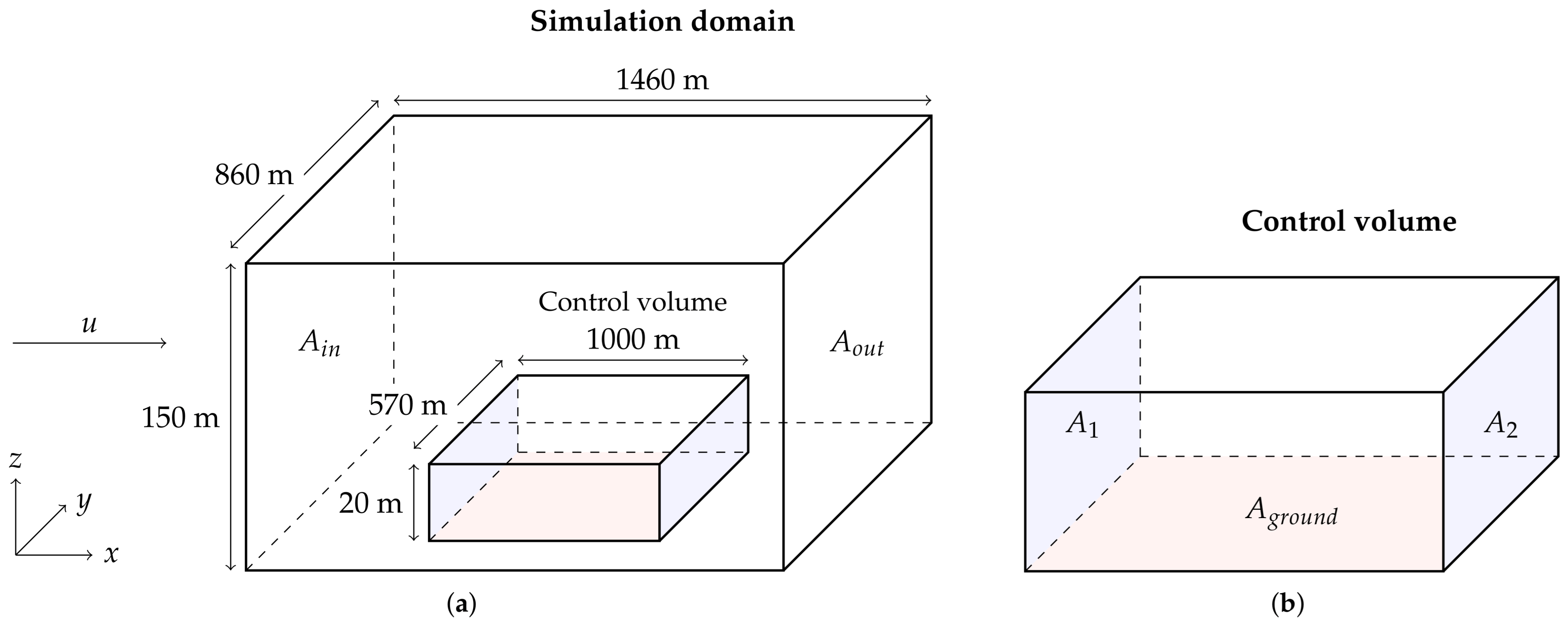
The numerical setup of the detailed simulation follows exactly the configuration presented in [7], ensuring direct comparability between roughness-based modeling and volumetric parameter-based modeling. The computational domain extends approximately $1.5\mathrm{km}\times 1.0\mathrm{km}$ horizontally, with a vertical extent of $0.15\mathrm{km}$. Realistic three-dimensional building geometries based on LoD2 data (from LGL Baden-Württemberg) are used to resolve the urban structure in detail. To focus on aerodynamic building effects, the terrain is modeled as a flat surface with a uniform roughness length of $z_0=0.01\mathrm{m}$ representing standard ground (Figure 1).

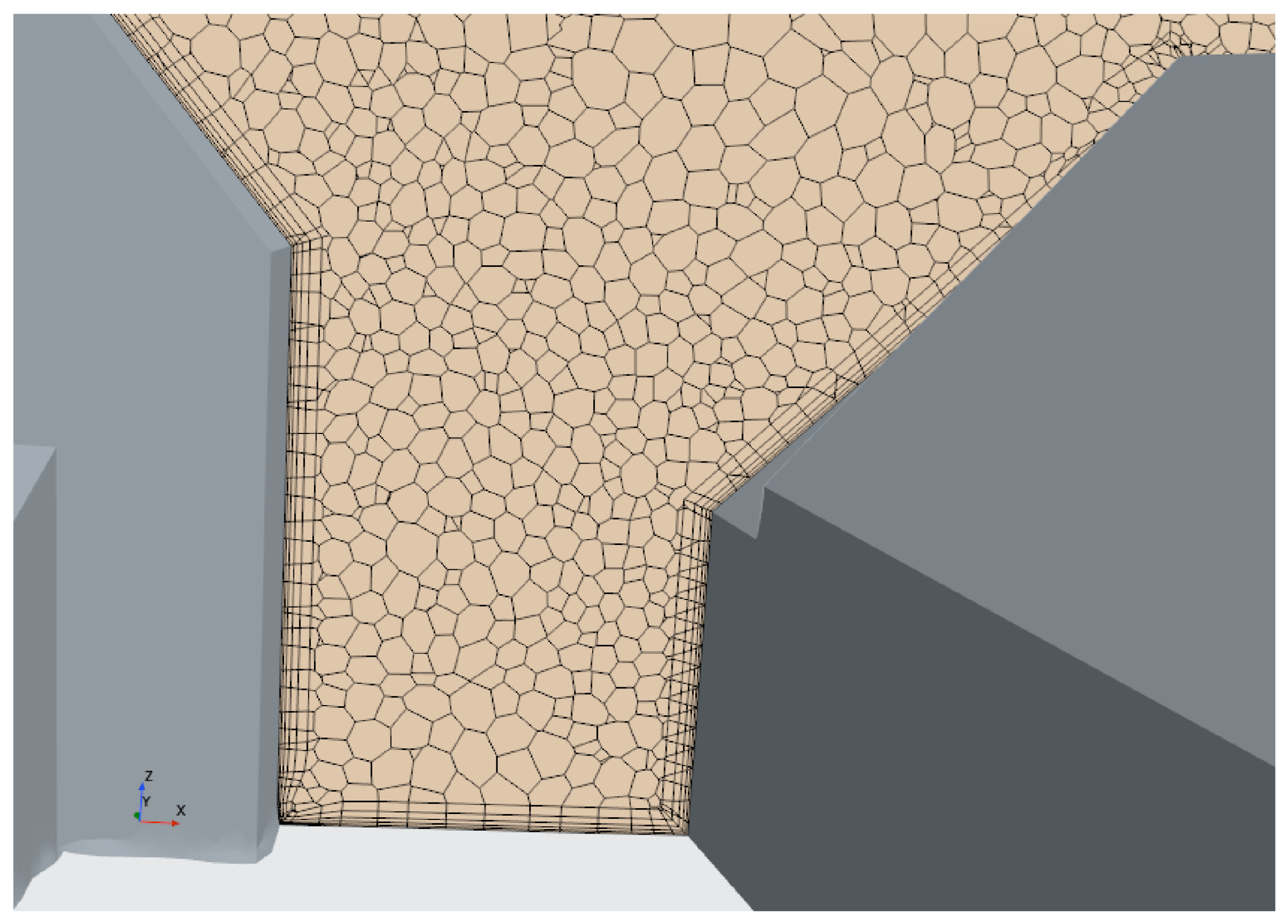
The mesh consists of polyhedral control volumes with prism layer refinement near solid boundaries (Figure 2). A high-$y^{+}$ wall treatment is applied, with $30<y^{+}<300$, ensuring adequate resolution of the logarithmic boundary layer while maintaining computational efficiency. A grid independence test is conducted, which shows that the grid used has no effect on the results.

All simulations are performed as steady-state and incompressible. Turbulence is represented using the k–$\omega$ SST model. To better represent atmospheric boundary layer conditions, the model constant ${\beta }^{🟉}$ is set to 0.03 (

Table 1. Turbulence coefficients for the modified $k-\omega$ turbulence model used in the canopy model.

${\mathit{\beta }}^{\mathbf{🟉}}$	${\mathit{C}}_{\mathit{ϵ}\mathbf{4}}$	${\mathit{C}}_{\mathit{ϵ}\mathbf{5}}$	${\mathit{\beta }}_{\mathit{p}}$	${\mathit{\beta }}_{\mathit{d}}$
$0.03$	$0.78$	$0.78$	$1.0$	$5.03$

) according to [13]. A logarithmic velocity profile is imposed at the inlet to represent a fully developed turbulent boundary layer, with flow aligned in the positive x-direction. Gravitational acceleration is included, while thermal stratification effects are neglected due to the limited vertical domain extent. Further details on domain setup, meshing strategy, and boundary conditions are provided in [7].

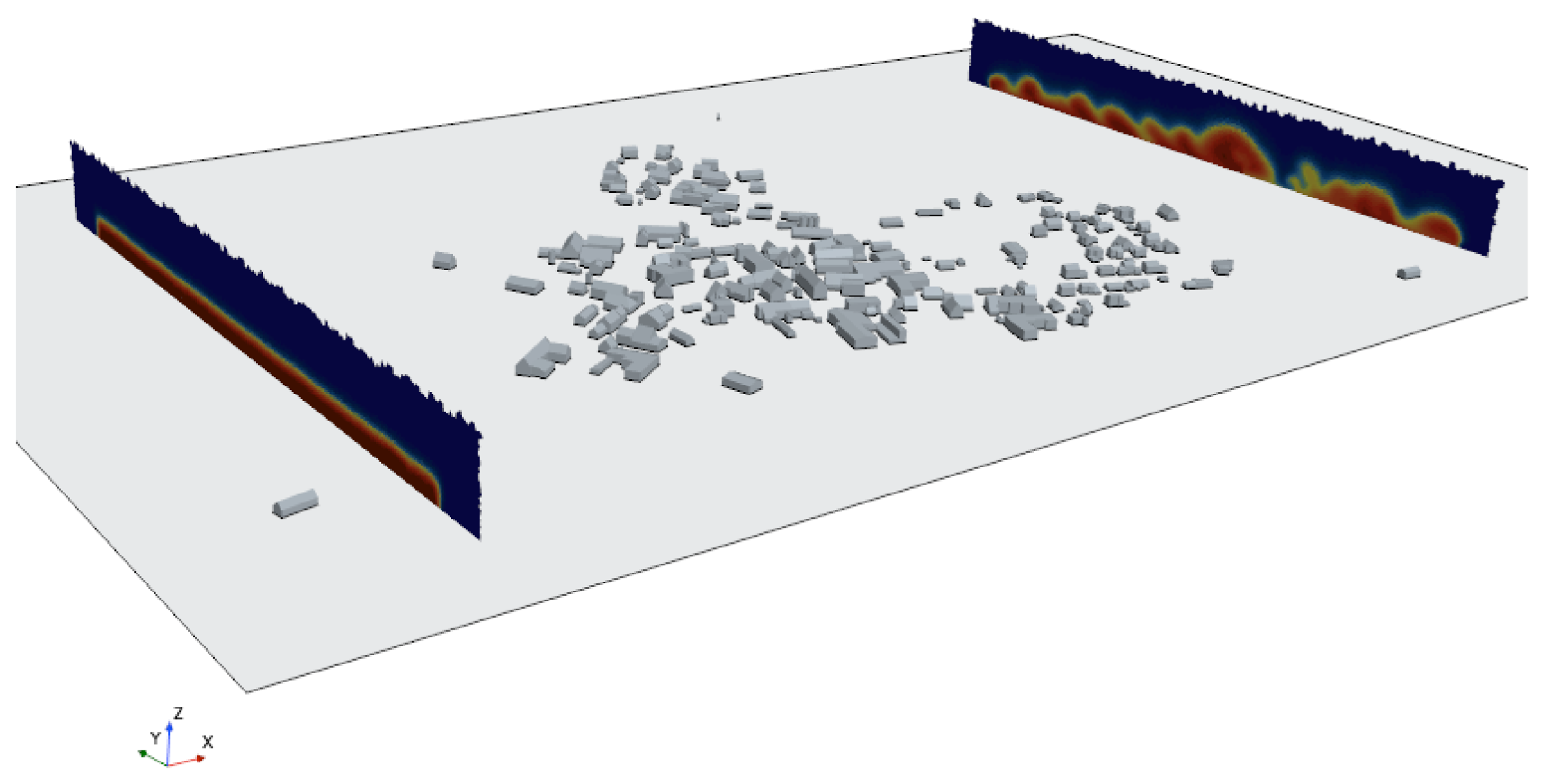
Following the further development of the evaluation method to assess the momentum balance over a control volume (see Section 2.3), a rectangular control volume aligned to the direction of flow is utilized for the evaluation of the urban structure (Figure 3). Since the control volume is aligned to the direction of flow, the momentum balance can be simplified using the three boundaries $A_1$, $A_2$, and $A_{ground}$. Since the flow decelerates and expands as it passes through the urban structure (as demonstrated later in Section 3.1), the area $A_2$ is adjusted so that the entire mass flow that passed $A_1$ also directly passes $A_2$. A passive scalar was used to precisely determine the shape and size of $A_2$. Passive scalars have no physical interaction with the flow, no mass, and no volume. They can serve as markers that, in this case, flow through the simulation area only by convection [14]. The passive scalars used in this work as markers have numerical values that are set to one at area $A_1$ in this simulation, and otherwise zero.

2.2. Formulation of the Urban Canopy Model

For the formulation of the urban canopy model the Reynolds-averaged Navier–Stokes (RANS) momentum equation is considered:

$${\displaystyle \frac{\partial \left(\rho \underline{u}\right)}{\partial t}}+\nabla ·(\rho \underline{u}\otimes \underline{u})=-\nabla p+\nabla ·\underset{=}{\tau }+\rho \underline{f}$$

(1)

In meso-scale simulations, urban geometries cannot be resolved explicitly and must therefore be parameterized. In the presented approach, the influence of unresolved urban structures is represented by an additional volumetric source term $\underline{S_u}$, yielding:

$${\displaystyle \frac{\partial \left(\rho \underline{u}\right)}{\partial t}}+\nabla ·(\rho \underline{u}\otimes \underline{u})=-\nabla p+\nabla ·\underset{=}{\tau }+\underline{S_u}$$

(2)

$\underset{=}{\tau }$ includes both viscous and Reynolds stresses. The Reynolds stress term $-\rho \overline{{\underline{u}}^{\prime }\otimes {\underline{u}}^{\prime }}$ is closed using the k-$\omega$ SST turbulence model, which is widely applied for wall-bounded and separated flows due to its robustness and accuracy [15,16]. The additional canopy source terms introduced in the present work act on the mean flow and turbulence transport equations but do not modify the underlying turbulence closure.

The introduction of volumetric drag terms follows established approaches for vegetated canopies, where unresolved obstacles are represented as distributed momentum sinks [8,9,13,17]. Similar formulations have also been applied in urban canopy modeling [10], although typically with empirically prescribed parameters.

In analogy to these approaches, the urban region is represented in the momentum equation in the same way as a porous medium, and the momentum sink is modeled as:

$$\underline{S_u}=-\rho c_d\mathrm{HAD}\left(z\right)\left|\underline{u}\right|\underline{u}$$

(3)

This formulation is consistent with established plant canopy drag laws, in which the drag force is proportional to the local dynamic pressure and a geometric density parameter [17]. In plant canopy models, this density is commonly expressed as Leaf Area Density (LAD) [8], whereas in the present work it is redefined as House Area Density (HAD) to represent the urban morphology.

In addition to the momentum equation, the transport equations for turbulent kinetic energy k and turbulent specific dissipation rate $\omega$ are modified by additional source terms following established canopy turbulence closures [13,17]:

$$\begin{array}{c}{S}_k=\rho c_d\mathrm{HAD}\left({\beta }_p|\underline{u}{|}^3-{\beta }_{d}k\left|\underline{u}\right|\right)\end{array}$$

(4)

$$\begin{array}{c}{S}_{\omega }=\rho c_d\mathrm{HAD}{\displaystyle \frac{\omega }{k}}\left(C_{\epsilon 4}{\beta }_p|\underline{u}{|}^3-C_{\epsilon 5}{\beta }_{d}k\left|\underline{u}\right|\right)\end{array}$$

(5)

These terms describe the conversion of mean kinetic energy, as obtained from the momentum equation, into the transport equations of the turbulent quantities k and $\omega$, driven by wake production and shear effects within the urban canopy. Accordingly, the source terms $S_k$ and $S_{\omega }$ consist of a production and a dissipation contribution. The associated model coefficients ${\beta }^{🟉},C_{ϵ4},C_{ϵ5},{\beta }_p,$ and ${\beta }_d$ are adopted from [13] (summarized in Table 1), where they were originally formulated within a k–$\epsilon$ framework. In the present study, these coefficients are mapped to their corresponding counterparts in the k–$\omega$ formulation (e.g., $C_{\mu }$ to ${\beta }^{🟉}$), assuming consistency between the underlying turbulence closure concepts. This approach is justified by the structural analogy between vegetation and urban canopies, as both can be represented as porous media that induce momentum loss and turbulence production primarily through drag-induced wake generation and shear at the obstacle scale. Consequently, the dominant mechanisms governing turbulence production and dissipation are comparable, allowing the use of established canopy-model coefficients as a first-order approximation. Furthermore, since the objective of this study is not to resolve detailed turbulence structures but to obtain reliable predictions of mean flow quantities such as velocity and pressure fields, the use of a simplified canopy parameterization based on plant canopy models is considered sufficient and computationally efficient.

The formulation relies on the following assumptions:

(i)

The urban canopy is conditioned as a homogenized medium at the grid scale, analogous to porous medium.

(ii)

Drag forces are aligned with the local velocity vector (isotropic resistance).

(iii)

The drag coefficient $c_d$ is spatially constant within the urban canopy.

(iv)

The urban geometric morphology is fully represented by the vertical distribution of HAD.

While the mathematical structure of the source terms follows established canopy modeling approaches, the key difference lies in the parameter identification strategy. In contrast to existing studies where drag coefficients and density functions are prescribed or empirically derived, all model parameters are obtained directly from detailed building-resolving CFD simulations of real urban geometries.

2.3. Derivation of the House Area Density and a Drag Coefficient

In the case of urban geometries the leaf area density $\alpha$ (LAD) of [13] can be reinterpreted as House Area Density (HAD). The ability to evaluate the density distribution at any height directly from the three-dimensional geometry data makes the determination via leaf area index (LAI) and generic distribution functions obsolete. With regard to Equations (3)–(5) the house area density (HAD) and the drag coefficient $c_d$ are the two unknown parameters. They are the key parameters for adjusting the urban canopy model derived in this study. In this context, the HAD is used as a parameter that represents the geometric distribution of urban geometry, whereas the drag coefficient provides information about the influence on the flow. The HAD is defined as the projected built-up area per unit volume in the vertical (z) direction. For its computation, the projected building area is evaluated in horizontal slices with a vertical resolution of $1\mathrm{m}$. Within each height interval, the building area is projected onto a horizontal plane, yielding the built-up area. The corresponding volume is defined as the horizontal extent of the urban domain multiplied by the height increment $\Delta z=1\mathrm{m}$. The HAD is then obtained as the ratio of projected area to volume for each height level. The vertical distribution of HAD is computed from ground level up to a height of $20\mathrm{m}$. To determine the source term $\underline{S_u}$ the momentum balance of the control volume (Equation (6)) is analyzed. The involved terms, which represent the relevant forces, are determined. The gravitational force was omitted from the momentum balance, as the air in this simulation can be considered incompressible [7].

$$\begin{array}{cc}\hfill {\int }_{\partial V}\rho \underline{u}(\underline{u}·\underline{n})\mathrm{d}A& =\sum _i\underline{F_i}\hfill \end{array}$$

(6)

$$\begin{array}{cc}\hfill {\int }_{\partial V}\rho \underline{u}(\underline{u}·\underline{n})\mathrm{d}A& ={\int }_{\partial V}\underset{=}{\sigma }\underline{n}\mathrm{d}A+{\int }_V\rho \underline{f}\mathrm{d}V\hfill \end{array}$$

(7)

$$\begin{array}{cc}\hfill {\int }_{\partial V}\rho \underline{u}(\underline{u}·\underline{n})\mathrm{d}A& =-{\int }_{\partial V}p\underline{n}\mathrm{d}A+{\int }_{\partial V}\underset{=}{\tau }\underline{n}\mathrm{d}A+{\int }_V\underset{\underline{S_u}}{\underbrace{\rho \underline{f}}}\mathrm{d}V\hfill \end{array}$$

(8)

$$\begin{array}{cc}\hfill {\int }_V\underline{S_u}\mathrm{d}V& =\underset{M}{\underbrace{{\int }_{\partial V}\rho \underline{u}(\underline{u}·\underline{n})\mathrm{d}A}}+\underset{P}{\underbrace{{\int }_{\partial V}p\underline{n}\mathrm{d}A}}-\underset{T}{\underbrace{{\int }_{\partial V}\underset{=}{\tau }\underline{n}\mathrm{d}A}}\hfill \end{array}$$

(9)

In the following the momentum flow through the control surface is denoted by M, the pressure force on the control surface by P and the friction force on the wall by T.

In order to substitute Equation (3) into Equation (9), Equation (3) has to be integrated, with $\rho$ and $c_d$ assumed to be constant.

$$\begin{array}{cc}\hfill {\int }_V\underline{S_u}\mathrm{d}V& ={\int }_V-\rho c_d\mathrm{HAD}\underline{u}\left|\underline{u}\right|\mathrm{d}V\hfill \end{array}$$

(10)

$$\begin{array}{cc}\hfill {\int }_V\underline{S_u}\mathrm{d}V& =-\rho c_d\underset{Q}{\underbrace{{\int }_V\mathrm{HAD}\underline{u}\left|\underline{u}\right|\mathrm{d}V}}\hfill \end{array}$$

(11)

Now, Equation (11) can be solved for $c_d$ and Equation (9) can be substituted. For a better overview, the previously defined symbols are used in Equation (14).

$$\begin{array}{cc}\hfill c_d& =-{\displaystyle \frac{{\displaystyle {\int }_V\underline{S_u}\mathrm{d}V}}{{\displaystyle \rho {\int }_V\mathrm{HAD}\underline{u}\left|\underline{u}\right|\mathrm{d}V}}}\hfill \end{array}$$

(12)

$$\begin{array}{cc}\hfill c_d& =-{\displaystyle \frac{{\displaystyle {\int }_{\partial V}\rho \underline{u}(\underline{u}·\underline{n})\mathrm{d}A+{\int }_{\partial V}p\underline{n}\mathrm{d}A-{\int }_{\partial V}\underset{=}{\tau }\underline{n}\mathrm{d}A}}{{\displaystyle \rho {\int }_V\mathrm{HAD}\underline{u}\left|\underline{u}\right|\mathrm{d}V}}}\hfill \end{array}$$

(13)

$$\begin{array}{cc}\hfill c_d& =-{\displaystyle \frac{M+P-T}{\rho ·Q}}\hfill \end{array}$$

(14)

This formulation allows the direct determination of $c_d$ from post-processing data of detailed building-resolving CFD data without the need to determine empirical parameters, correlations or calibration. The resulting drag coefficient $c_d$ represents an effective bulk parameter that captures the total aerodynamic impact of the urban region in meso-scale flow simulation in a physically consistent manner. In addition, the height distribution of the buildings is represented be the parameter HAD in a geometrically consistent manner.

2.4. Model Implementation in STAR-CCM+ 2406

Simcenter STAR-CCM+ offers the option of defining momentum source terms and turbulence source terms for regions. These source terms can be related to field functions that dynamically determine the value of the source term. For the momentum source term, Equation (3) is used as a field function and set as the momentum source in the region that incorporates the urban region. Analogously, Equations (4) and (5) are set as source terms for k and $\omega$. The HAD distribution is derived from the urban geometry using a table and a field function based on this table.

As visualized in Figure 3, the model is extended to the same dimensions as for the evaluation of the momentum balance. This consistency is important because the momentum balance provides an effective force for a control volume, on the basis of which the drag coefficient is calculated.

3. Results

This section presents the results of the derivation of the HAD and of the $c_d$ from the detailed simulation. The simulation results are then compared with the results of the simulation using the urban canopy model. As described in [7], computational analyses within this study also showed that the mesh resolution has no effect on the resulting parameters. Furthermore, enlarging the simulation domain in front of the urban region does not show any influence on the results.

3.1. Results of the Detailed Simulation

The detailed simulation has a size of approximately 44.7 million cells with refinement towards the ground and urban geometry. The total CPU time required for 1.500 iterations is 122.5 CPU-hours.

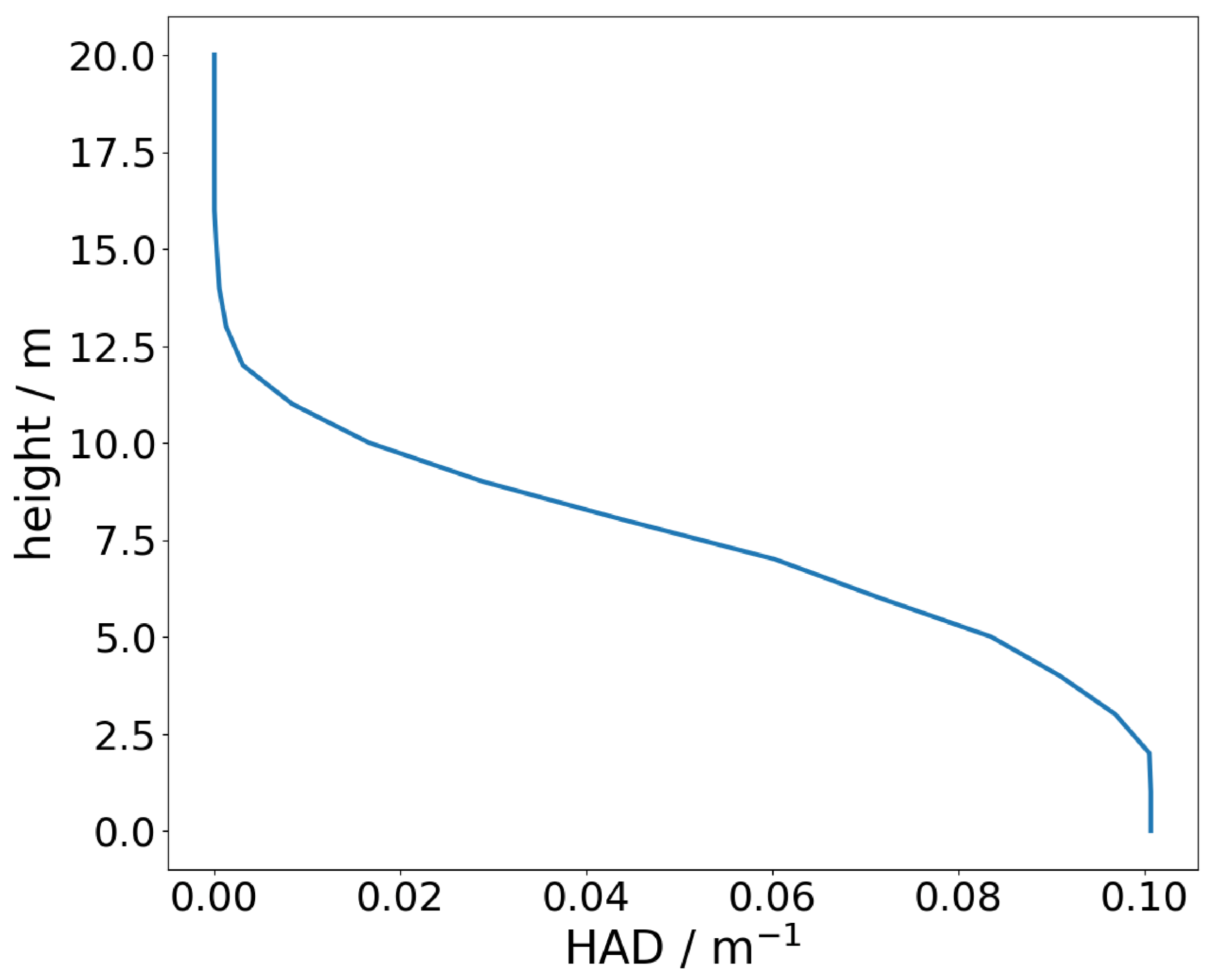
The HAD distribution used for post-processing of any data and used in any meso-scale simulations was derived from the LoD2 data (from LGL Baden-Württemberg) of Stötten, a flat terrain near the WINSENT wind research test site in the Swabian Albs close to Geislingen an der Steige, Baden-Württemberg, Germany (48.652733, 9.859998), within the control volume. To calculate the distribution functions, the projected area in the vertical direction was determined for height sections of one meter. The exact process for determining the HAD is described in Section 2.3. This results in the HAD being identified as the projected area per unit volume. The values vary from $0.1$ at ground level to 0 at a height of approximately 15 m (see Figure 4). Due to the rural geographical location, there are several smaller sheds in Stötten, which explains the beginning of the decrease in the HAD at heights of only 2.5 m.

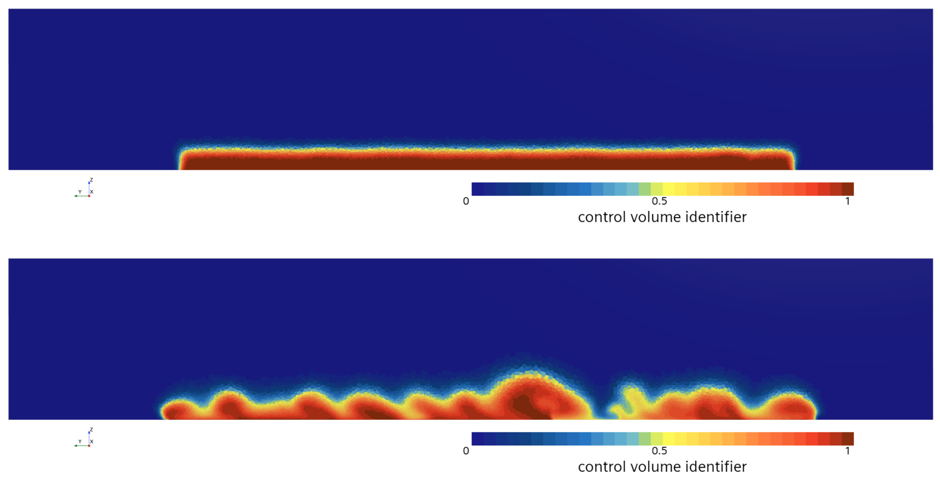
The momentum balance is evaluated in the control volume between areas $A_1$ and $A_2$ as described in Section 2.1. A passive scalar is set to one to define a part of the entire simulation domain. This passive scalar has no influence on or interaction with the physical modeling in the simulation. It is solely a post-processing parameter. This passive scalar is called a control volume identifier. The purpose of the control volume identifier is to define a flow conduit which allows us to post-process momentum terms and other physical quantities within the flow conduit. Figure 5 shows two cross-sections within the entire simulation domain in the flow direction at the level of areas $A_1$ and $A_2$. It is important to note that areas $A_1$ and $A_2$ include the areas highlighted in red by the control volume identifier. To evaluate the momentum balance, the three terms in the numerator of Equation (14) (M, P, and T) as well as the denominator (Q) are obtained from the detailed CFD simulation including the full urban geometry. These quantities are evaluated separately for the streamwise, lateral, and vertical directions (x, y and z, respectively). The results are shown in

Table 2. Results of the momentum balance based on the detailed simulation.

Detailed Simulation
Momentum Term	Upstream (${\mathit{A}}_{\mathbf{1}}$)	Downstream (${\mathit{A}}_{\mathbf{2}}$)	Balance
$M_x$	4.4 · 105	3.9 · 105	−5.0 · 104
$P_x$	−1.3 · 106	−2.3 · 106	−9.6 · 105
$T_x$			−1.7 · 104
$Q_x$			5.6 · 107
$M_y$	1.7 · 103	−4.6 · 103	−6.3 · 103
$P_y$	−1.3 · 106	−2.3 · 106	−9.6 · 105
$T_y$			−7.6 · 102
$Q_y$			−5.3 · 105
$M_z$	2.5 · 102	−9.6 · 102	−1.2 · 103
$P_z$	−1.3 · 106	−2.3 · 106	−9.6 · 105
$T_z$			−4.8 · 102
$Q_z$			−9.7 · 104

$M_i$, $P_i$, and $T_i$ are given in $\mathrm{N}$; $Q_i$ is given in ${\mathrm{m}}^4{\mathrm{s}}^{-2}$.

. It can be seen by the significant change in $M_y$ and $M_z$ that the momentum flow is significantly deflected in the lateral and vertical directions by the urban geometry. Comparative calculations without urban geometry and without an active urban canopy model result in momentum flows of $2.110·{10}^2\mathrm{N}$ in the lateral and vertical directions, which are of significantly lower value. Since static pressure is a scalar quantity, it is independent of the direction of evaluation, which is also reflected in the results. The calculation of $c_d$ is performed based on the terms of the main flow direction x: $M_x$, $P_x$ and $T_x$. The calculation is shown in Equation (15).

$$c_d=-{\displaystyle \frac{M_x+P_x-T_x}{\rho ·Q_x}}=-{\displaystyle \frac{-4.975·{10}^4\mathrm{N}-9.611·{10}^5\mathrm{N}+1.452·{10}^5\mathrm{N}}{1.2\frac{\mathrm{kg}}{{\mathrm{m}}^3}·5.600·{10}^7\frac{{\mathrm{m}}^4}{{\mathrm{s}}^2}}}\approx 0.015$$

(15)

The relatively low value of the drag coefficient arises from its definition within the canopy parameterization and should not be interpreted as the drag coefficient of an individual building. In the present formulation, $c_d$ represents an effective (bulk) drag coefficient that is coupled with the canopy morphology through the parameter $\mathrm{HAD}$, meaning that the total drag force is distributed over the entire control volume rather than being associated with discrete obstacles. Therefore, $c_d$ should be understood as a model coefficient within a porous-medium representation of the urban canopy, rather than a physical drag coefficient of individual buildings. Its magnitude is consistent with this formulation and does not indicate an underestimation of drag forces.

3.2. Results of the Urban Canopy Model

The urban canopy simulation has a size of approximately 14.9 million cells with refinement towards the ground. The total CPU time required for 1.500 iterations is 40.4 CPU-hours.

To validate the reliability of the urban canopy model and the process of the derivation of the parameters HAD and $c_d$, CFD simulations were performed using the momentum sources based on the urban canopy model. The detailed geometry of the urban region is not resolved in the computational domain here.

The momentum balance was evaluated for the streamwise (x), lateral (y), and vertical (z) directions by comparing the contributions from momentum flow M, pressure forces P, and friction forces T. The results are shown in

Table 3. Results of momentum balance based on the urban canopy model.

Urban Canopy Model
Momentum Term	Upstream (${\mathit{A}}_{\mathbf{1}}$)	Downstream (${\mathit{A}}_{\mathbf{2}}$)	Balance
$M_x$	4.5 · 105	4.0 · 105	−5.1 · 104
$P_x$	−1.4 · 106	−1.9 · 106	−4.9 · 105
$T_x$			−3.6 · 103
$M_y$	6.9 · 101	−2.7 · 100	−7.2 · 101
$P_y$	−1.4 · 106	−1.9 · 106	−4.9 · 105
$T_y$			−1.2 · 101
$M_z$	3.9 · 102	−10.0 · 103	−1.4 · 103
$P_z$	−1.4 · 106	−1.9 · 106	−4.9 · 105
$T_z$			−4.0 · 10−11

$M_i$, $P_i$, and $T_i$ are given in $\mathrm{N}$.

. The momentum flow balance is strongly dominated by the streamwise component. With $M_x=-5.118·{10}^4\mathrm{N}$, the x-component exceeds the transverse components $M_z=-1.384·{10}^3\mathrm{N}$ and $M_y=-7.205·{10}^1\mathrm{N}$ by roughly one and three orders of magnitude, respectively ($\left|M_x\right|\gg \left|M_z\right|\gg \left|M_y\right|$).

In the streamwise direction, both models show very similar momentum flow balances. The detailed simulation yields $M_x=-4.975·{10}^4\mathrm{N}$, while the urban canopy model gives $M_x=-5.118·{10}^4\mathrm{N}$, corresponding to a difference of only about 3%. The pressure force is the dominant contribution in both cases. The pressure balance is $-9.611·{10}^5\mathrm{N}$ in the detailed simulation compared to $-4.897·{10}^5\mathrm{N}$ in the urban canopy model, indicating a substantially weaker pressure gradient in the urban canopy representation. Friction forces are comparatively small in both cases, with $-1.706·{10}^4\mathrm{N}$ in the detailed simulation and $-3.640·{10}^3\mathrm{N}$ in the urban canopy model. This reflects the explicit wall-resolved drag in the detailed geometry, whereas the urban canopy parameterization produces a significantly smaller net friction contribution.

In the lateral direction, the models show pronounced differences. The detailed simulation has a momentum flow balance of $M_y=-6.314·{10}^3\mathrm{N}$, whereas the urban canopy model yields only $M_y=-7.205·{10}^1\mathrm{N}$. Thus, the lateral momentum flow in the urban canopy model is reduced by nearly two orders of magnitude. Friction forces are again considerably larger in the detailed simulation ($-7.612·{10}^2\mathrm{N}$) than in the urban canopy model ($-1.173·{10}^1\mathrm{N}$), indicating that the resolved urban geometry induces substantially stronger lateral momentum exchange.

In the vertical direction, the momentum flow balances are of similar magnitude in both models. The detailed simulation yields $M_z=-1.209·{10}^3\mathrm{N}$, while the urban canopy model yields $M_z=-1.384·{10}^3\mathrm{N}$. The friction force differs strongly between the models: the detailed simulation predicts $-4.805·{10}^2\mathrm{N}$, whereas the urban canopy model shows a nearly negligible contribution (≈$0\mathrm{N}$). This indicates that vertical momentum transfer through wall shear is largely absent in the parameterized canopy representation. However, differently to the detailed simulation, the deflection of the momentum flow in the lateral direction is very low, whereas the deflection in the vertical direction is increased. This is due to the HAD distribution, which shows a maximum at the ground and decreases upwards. As a result, the flow is deflected upwards. In terms of magnitude, the urban canopy model slightly overestimates the momentum flow loss. At the same time, the pressure force is underestimated. Despite these discrepancies, the overall momentum balance remains physically consistent. In particular, the dominant streamwise component is captured with adequate accuracy. The level of agreement is therefore considered sufficient for the intended application.

4. Discussion

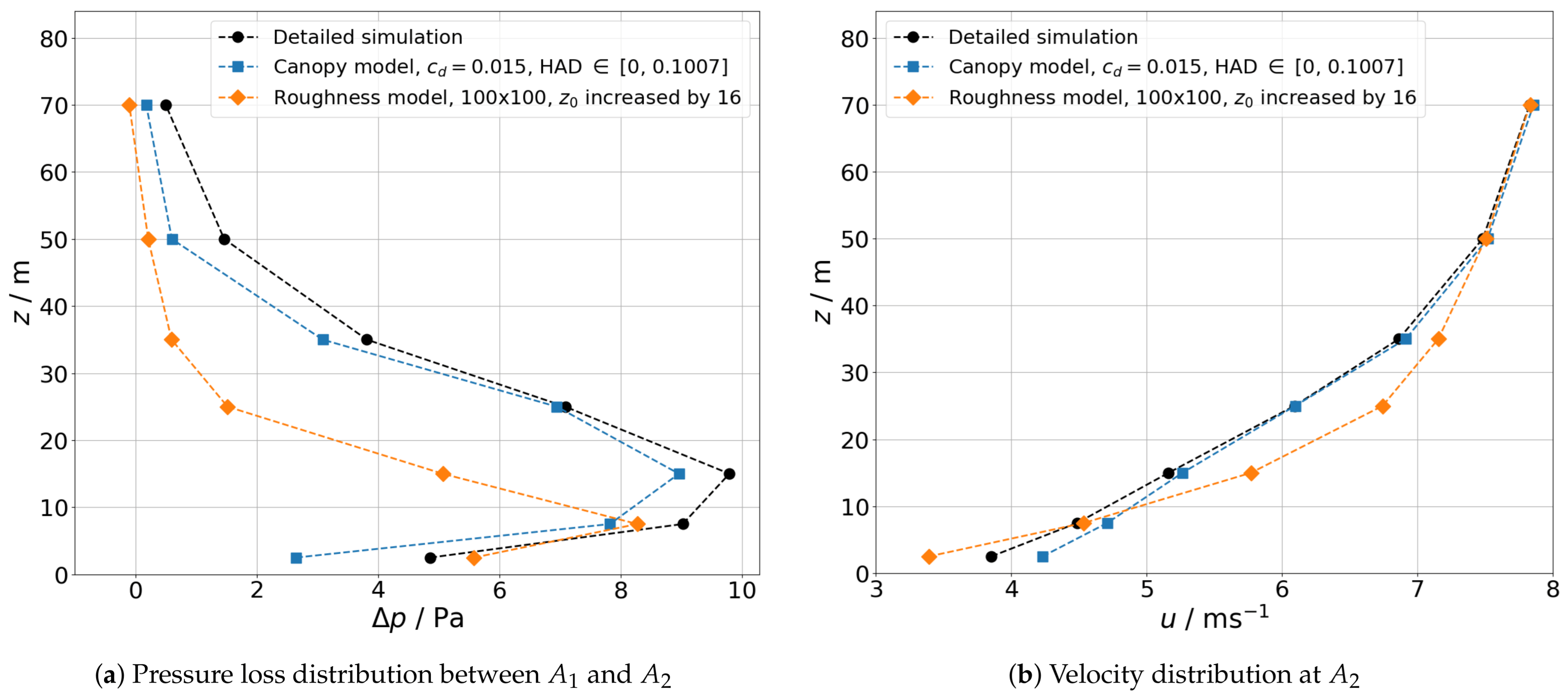
The agreement of the terms of the momentum balance is a very ambitious criterion for the validation of the urban canopy model. With respect to the usage of the urban canopy model in meso-scale CFD simulations, a correct representation of the pressure losses over the height of urban regions represents the relevant outcome of the model. Therefore, the pressure loss distribution over the height of the urban region is considered for the validation of the urban canopy model. Furthermore, the velocity distribution over the height in the urban region is another significant quantity in the meso-scale simulations. Thus, the velocity distributions of the detailed simulation and of the urban canopy model are compared. Additionally, the results of simulations using a conventional roughness model are compared with the two previously mentioned models to allow us to evaluate the performance of the newly presented modeling approach [7]. Figure 6a denotes the area-averaged pressure loss between the areas $A_1$ and $A_2$, which are used again for this evaluation. As shown in Figure 6a, the pressure loss is well represented by the urban canopy model in comparison to the detailed simulation. The distribution of pressure loss is represented with greater accuracy than in the roughness models, as the latter are unable to properly reflect the qualitative progression and significantly underestimate pressure losses at heights above 10 m. Despite the substantial agreement between the urban canopy model and the detailed simulation, there are minor discrepancies in the results. In addition to the pressure loss distribution, the area-averaged velocity distribution of the urban canopy model at $A_2$ (Figure 6b) also demonstrates a substantial enhancement in comparison to the roughness model. In this case, the velocities under 10 m are marginally overestimated, while the roughness model underestimates them. Conversely, the average velocities of the detailed simulation and the urban canopy model exhibit strong agreement, while the roughness model significantly overestimates the average velocities from a height of 10 m to 40 m. Thus, the roughness model does not achieve sufficient deceleration of the flow.

It should further be noted that the validation case considered in this study is based on a rural, flat terrain with sparse and low-rise buildings. This setup reflects the application context of meso-scale wind energy site assessments, such as within the WINSENT project, where small settlements are of primary interest. Within this scope, the proposed approach is particularly suitable for representing small towns and rural environments in meso-scale simulations. However, the transferability of the derived parameters and the model performance for dense urban areas with higher building densities and more complex morphologies has not yet been assessed. While no fundamental conceptual limitations of the volumetric formulation are anticipated, further validation and potential model extensions, such as anisotropic drag formulations or direction-dependent density functions, may be required to accurately represent complex urban environments.

5. Conclusions

The results presented in this study indicate that the urban canopy model offers a significant reduction in the computational effort required for simulations in meso-scale site assessments. The utilization of the urban canopy model, which was developed in this study, resulted in a reduction of two-thirds in both the number of cells and the total CPU time. However, the urban canopy model cannot reflect the exact results of the momentum balance.

The results of the urban canopy model show a strong correspondence with the results of the detailed simulation and significantly outperform the results of the roughness model. The urban canopy model’s structural design, which is based on the existing and established canopy models, has the potential to result in a more uniform approach within the domain of volumetric canopy models. Furthermore, the division of geometric properties and resistance effects into HAD and $c_d$ provides the same modeling degrees of freedom as conventional canopy models.

Nevertheless, there is still potential for improvement in order to get the urban canopy model even closer to the results of the detailed simulation. First of all, there is the pure deflection of the momentum flow in the vertical direction, which the HAD cannot accurately represent. In this context, the implementation of individual source terms for the x, y, and z directions is a feasible and promising approach. These could be implemented via an additional HAD distribution function for the longitudinal and lateral directions.

In addition, the significant underestimation of the friction force terms could be compensated for by superimposing the roughness model. This could potentially also narrow the gap of the velocity distribution under 10 m.

References

- Castellani, F.; Astolfi, D.; Mana, M.; Piccioni, E.; Becchetti, M.; Terzi, L. Investigation of Terrain and Wake Effects on the Performance of Wind Farms in Complex Terrain Using Numerical and Experimental Data. Wind Energy 2017, 20, 1277–1289. [Google Scholar] [CrossRef]
- El Bahlouli, A.; Leukauf, D.; Platis, A.; zum Berge, K.; Bange, J.; Knaus, H. Validating CFD Predictions of Flow over an Escarpment Using Ground-Based and Airborne Measurement Devices. Energies 2020, 13, 4688. [Google Scholar] [CrossRef]
- Grimmond, C.S.B.; Oke, T.R. Aerodynamic Properties of Urban Areas Derived from Analysis of Surface Form. J. Appl. Meteorol. 1999, 38, 1262–1292. [Google Scholar] [CrossRef]
- Lettau, H. Note on Aerodynamic Roughness-Parameter Estimation on the Basis of Roughness-Element Description. J. Appl. Meteorol. 1969, 8, 828–832. [Google Scholar] [CrossRef]
- Raupach, M.R. Drag and Drag Partition on Rough Surfaces. Bound.-Layer Meteorol. 1992, 60, 375–395. [Google Scholar] [CrossRef]
- Macdonald, R.; Griffiths, R.; Hall, D. An Improved Method for the Estimation of Surface Roughness of Obstacle Arrays. Atmos. Environ. 1998, 32, 1857–1864. [Google Scholar] [CrossRef]
- Vögtle, M.; Stauch, R.; Knaus, H. Derivation of a Roughness Model for Urban Areas by Means of Detailed CFD Simulation. In Proceedings of the Advances in Computational Heat and Mass Transfer II; Cetin, B., Dursunkaya, Z., Günay, A.A., Gözükara, A.C., Eds.; Springer: Cham, Switzerland, 2026; pp. 385–395. [Google Scholar]
- Shaw, R.H.; Schumann, U. Large-Eddy Simulation of Turbulent Flow Above and Within a Forest. Bound.-Layer Meteorol. 1992, 61, 47–64. [Google Scholar] [CrossRef]
- Finnigan, J. Turbulence in Plant Canopies. Annu. Rev. Fluid Mech. 2000, 32, 519–571. [Google Scholar] [CrossRef]
- Otte, T.L.; Lacser, A.; Dupont, S.; Ching, J.K.S. Implementation of an Urban Canopy Parameterization in a Mesoscale Meteorological Model. J. Appl. Meteorol. 2004, 43, 1648–1665. [Google Scholar] [CrossRef]
- Salamanca, F.; Martilli, A.; Tewari, M.; Chen, F. A Study of the Urban Boundary Layer Using Different Urban Parameterizations and High-Resolution Urban Canopy Parameters with WRF. J. Appl. Meteorol. Climatol. 2011, 50, 1107–1128. [Google Scholar] [CrossRef]
- Jandaghian, Z.; Berardi, U. Comparing urban canopy models for microclimate simulations in Weather Research and Forecasting Models. Sustain. Cities Soc. 2020, 55, 102025. [Google Scholar] [CrossRef]
- Dalpé, B.; Masson, C. Numerical Study of Fully Developed Turbulent Flow Within and Above a Dense Forest. Wind Energy 2008, 11, 503–515. [Google Scholar] [CrossRef]
- Siemens Industries Digital Software. Simcenter STAR-CCM+ User Guide, version 2024. In Passive Scalar; Siemens: München, Germany, 2024; pp. 4027–4039. [Google Scholar]
- Menter, F.R. Two-equation eddy-viscosity turbulence models for engineering applications. AIAA J. 1994, 32, 269–289. [Google Scholar] [CrossRef] [PubMed]
- Menter, F.R.; Kuntz, M.; Langtry, R.B. Ten years of industrial experience with the SST turbulence model. AIAA J. 2003, 4, 625–632. [Google Scholar]
- Katul, G.G.; Mahrt, L.; Poggi, D.; Sanz, C. ONE- and TWO-Equation Models for Canopy Turbulence. Bound.-Layer Meteorol. 2004, 113, 81–109. [Google Scholar] [CrossRef]