Among the 17 patients listed in
Table 1, nine of them have symptoms and eight patients do not have symptoms. Therefore, we divide this section into two sections with results that differ from these conditions. According to the templates given in
Section 4.5, we calculate the coefficients
. According to the template given in
Section 4.2, we calculate the delay time parameter
. On the basis of
real measurements from 17 patients each, we loaded
base data
according the spline function
used to minimize (
9). Assuming it will be more understandable, we divide the section into four parts.
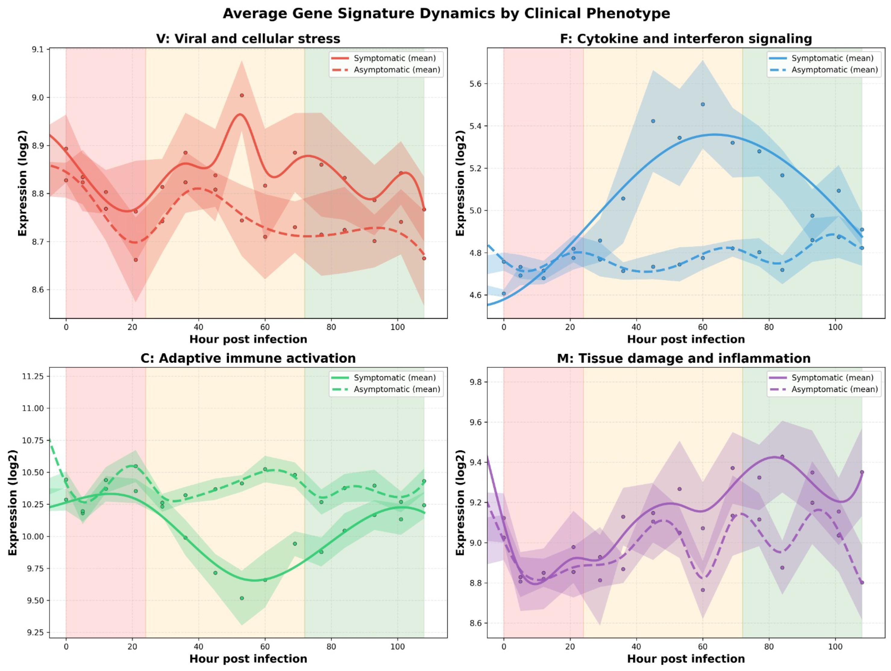
Several qualitative differences between the two clinical phenotypes are immediately visible. The viral stress signature exhibits sustained growth and elevated levels in symptomatic patients, whereas in asymptomatic individuals it remains comparatively stable and shows signs of suppression at later time points. In contrast, the innate immune response displays a pronounced delayed peak in symptomatic patients, while remaining smoother and less amplified in asymptomatic cases. The adaptive immune activation further highlights this divergence: asymptomatic patients demonstrate partial recovery toward baseline levels, whereas symptomatic patients show persistent deviation, indicating a failure of stabilization. Finally, the tissue damage signature exhibits substantial variability in both groups, with wide SEM intervals, suggesting weak direct observability and limited identifiability from transcriptomic data alone.
These phenotype-dependent differences are not imposed by the model but arise directly from the data. As shown in the following subsections, they provide a structural explanation for the distinct parameter regimes obtained during identification, including the emergence of delayed interactions, the necessity of additional background terms, and the differential reliability of parameter estimates across subsystems.
5.1. Asymptomatic Basic Results
We calculate the coefficients from Formula (
1) for transcriptomic latent states
and
:
According to Formula (
14), we proceed by Python [
33] programming codes and obtain the desired coefficients in (
35):
Until all coefficients have acceptable relative accuracy
and the problem is well-conditioned, the goodness of fit quantified by (
30) equals
, so the final conclusion is that the identification of the right-hand side in (
36) is not entirely reliable.
Analogously, we consider Formula (
15) for the transcriptomic latent states
and
, and we have:
According to Formula (
15), we proceed by Python programming codes and obtain the desired coefficients in (
39):
This time all coefficients have acceptable relative accuracy
and the problem is well-conditioned. Moreover, the goodness of fit quantified by (
30) equals
, so the identification of the right-hand side in (
40) is reliable. Finally, the condition number of the unregularized normal matrix calculated by (
34) is
, and the residual variance defined in (
31) equals
.
Next we take Formula (
17) without delay setting
for the transcriptomic latent states
and
, and we have:
According to (
18), we proceed, and obtain the coefficients in (
43):
This time no coefficient has acceptable accuracy, since one or more coefficients are poorly determined:
The goodness of fit
, so the coefficient estimation in (
44) is not reliable at all. The condition number
, so it is still well-conditioned.
Finally, for (4), for the transcriptomic latent states
and
, we have:
According to (
16), we proceed, and obtain the coefficients in (
47):
This is not as high as before, but now the coefficient accuracy is not acceptable, since
:
The goodness of fit measure
, meaning that the coefficient estimation in (
48) is not reliable. The condition number
indicates good condition.
5.2. Symptomatic Basic Results
In this subsection we calculate coefficients for the patients with expressed symptoms. Again, first we calculate the coefficients from Formula (
1) for transcriptomic latent states
and
:
According to (
14), we proceed with the programming codes and obtain the desired coefficients in (
51):
The coefficients have border accuracies
Until the problem is well-conditioned, since
, the goodness of fit of
is not sufficient for entire reliability. Note that the coefficients are similar to those obtained in (
35).
Analogously, Formula (2) gives, for
and
:
Formula (
15) and the Python algorithm codes give:
All coefficients have no acceptable relative accuracies
and the goodness of fit equals
, so the identification of the right-hand side in (
56) is not fully reliable. The condition
calculated by (
34) shows good conditioning, and residual variance
.
Taking (
17) without delay, with
for the transcriptomic latent states
and
, we have:
According to (
18), we proceed, and obtain the coefficients in (
43):
The coefficients are poorly determined:
The goodness of fit shows no reliability at all, and the condition number is well-conditioned still. Compared to the symptomatic case, there is an evident deviation.
Applying (4) for the transcriptomic latent states
and
, we have:
According to (
16), we proceed, and obtain the coefficients in (
63):
This is not so high as before, but now the coefficient accuracy is not acceptable, since
:
The goodness of fit of
implies an unreliable coefficient estimation in (
64). The condition number
indicates good condition.
5.3. Asymptomatic Extended Model Results
In these two subsections we extend the model given from (
1) to (4) with the mathematic tools presented in
Section 4.6, and considering
Section 4.4, where the values for
are proposed in (
27).
Since both (
36) and (
52) did not satisfy the reliability conditions with small
values, we propose to extend (
1) for latent states
and
with
To obtain
and
in (
67), we need to carry out as many iterations with as many
that are suggested in (
27). In
Table 3 the iterations are sorted by WMSE, calculated in (
28). Considering (
7) and (
8), we have different samples members’ numbers
for calculating the coefficients. In
Table 3,
and
are the weighted standard deviations used to normalize the regressors.
Finally we take
and
obtained for
, since in this case we have the smallest WMSE.
The coefficients have definitely acceptable relative accuracies:
In this case, , condition , and residual variance , so the RHS identification is reliable indeed.
By comparing (
67) with (
36), it is shown that there is no delay in both cases. The need for the additional parameter
suggests that some biological processes occur that are not explicitly represented in the original structure of the model. The negative parameter in the case of viral population expansion in (
68) is particularly interesting, as it indicates that something within the viral population causes extinction. First, we have only eight asymptomatic patients. It is possible that patients do not have disease symptoms precisely because of the negative coefficient
.
Enlarging (2), with delay and an additional parameter assumption, we have
Analyzing the coefficient fits for each
value given in (
27), we obtain
Table 4.
From
Table 4, we choose the coefficients given by
again, because they give the smallest coefficient
. We obtain the equation
The coefficients have acceptable relative accuracy:
The coefficient of determination shows that the regression model explains the variability of the dependent variable very well. The residual variance implies very high model precision. After , the problem is moderately ill-conditioned, and caution is advised.
When we enlarge (
17) for possible delays and an additional parameter, we get:
As before, calculating different
from (
27) entails
, with the best
, and the coefficients as follows:
In this case, we obtain coefficients with remarkable errors:
Moreover, shows that one or more coefficients are poorly determined. It is moderately ill-conditioned by , and RHS identification is not fully reliable until .
Related to (
44), the coefficients in (
78) are similar, and no delay is indicated. In particular,
is very significant in the sense that this simple Marchuk model does not cover asymptomatic patients.
Particularly, if we want to consider (
5)’s contribution to (
77), then we need to enlarge our coefficient analysis.
with
defined just as in (
5) somewhere above. In this case, we need a parallel
and
discussion, presented in the following
Table 5.
In
Table 5 the best results are
and
. In the sample created from
data by the spline given in (
9), we obtain the immune activation differential equation
with tissue damage function (
5):
Thanks to acceptable relative coefficient accuracies:
Together with the coefficients, from
Table 5, the goodness of fit is
, condition number
, and residual variance
, guaranteeing the reliability of Equation (
82)’s RHS identification.
Finally, transforming (4) to suppose a delay and taking an additional unused parameter for biological processes into account, we obtain the equation
Different from above, now we get through calculations, as presented in the next table.
From
Table 6, sorted by the value of
, we can find out the equation for the best
h.
Considering (
7) and (
8), we have a sample of
members for calculating coefficients with acceptable relative accuracies:
The high goodness of fit is given by , and the good predictive accuracy is given by . However, caution is advised since , so the problem is moderately ill-conditioned.
The negative coefficient indicates tissue’s tendency to ruin itself in the absence of a cure, since there are no symptoms.
5.4. Symptomatic Model Extension Results
Patients with explicit symptoms show different behaviors from the first Equation (
67). In contrast, we get contrasting results after analyzing
cases. After sorting by WMSE, from
Table 7, we obtain the optimal
h.
For symptomatic patients, Equation (
68) now reads as
Both coefficients have acceptable relative accuracy:
Good fitting is implied by , and good conditioning by . Additionally, , and RHS identification is reliable.
Related to (
68), symptomatic patients have a positive virus propagation coefficient, as expected, so this might have caused their symptoms.
Considering (
72) for the patient with symptoms, again we discuss the results for the different
values proposed in (
27).
In contrast with
Table 7, the
column in
Table 8 is not ordered the same way, but the best is still
h. For patients with symptoms, Equation (
73) turns into
Over the
data created, all coefficients
,
, and
have acceptable relative accuracies:
Finally we conclude that RHS identification is reliable, since high determination fixes the goodness of fit at , the well condition number at , and small residual variance at .
When relating (
96) with (
73), it is noticeable that in patients with symptoms, there is a positive cytokine dynamic dependence on surplus in adaptive immune activation in delay, in contrast with patients without symptoms. Meanwhile, the cytokines increase following their struggle with viruses in both cases.
Next, we find out the adaptive immune activation behavior when patients have disease symptoms. In this case, (
78) become
since the best
after we sort the coefficient calculations by
in
Table 9.
Coefficient relative accuracies are obviously acceptable:
The final conclusion is that RHS identification is reliable, which is a consequence of high determination, and good conditioning, , and strictness, .
The patients have symptoms since there is a delay in the body’s reaction. In contrast to (
78), here, the immune reaction increases with the struggle between cytokines and viruses, with higher immune activity.
A tissue damage and inflammation impact in (
100) is obtained by calculating the coefficients in (
82). Similarly to
Table 5, we use
Table 10.
From
Table 5, the immune activation equation reads
with tissue damage behavior
This is obtained for the best choice
and
from the sample created from
items. The coefficients
are of acceptable relative accuracies. The fit goodness is
, along with an acceptable condition number
and suitable residual variance
, implying that RHS identification is reliable.
If we relate (
104) to asymptomatic (
104), we recognize symptom absence by increasing the immune activity with the increasing struggle with viruses after 21 days. In contrast, patients with symptoms lose immune activity in the struggle and get immunity from an increase in cell density in the blood.
Finally, we calculate the coefficients in (
87) for patients with symptoms. The
grid results are sorted by WMSE in
Table 11.
The best
choice leads to a sample with
items and gives the equation
with acceptable relative accuracies
Once more, the determination coefficient is high and residual variance indicates high dependence on residuals. But, the condition number warrants caution of moderately ill-conditioned RHS identification, since it is not fully reliable.
Unlike asymptomatic patients, symptomatic patients take medication that helps keep tissues out of the risk zone defined by (
5).