Article

ECG Heartbeat Classification Using Echo State Networks with Noisy Reservoirs and Variable Activation Function


by
Ioannis P. Antoniades
1,
Anastasios N. Tsiftsis
1,
Christos K. Volos
1,
Andreas D. Tsigopoulos
2,*,
Konstantia G. Kyritsi
1 and
Hector E. Nistazakis
3
1
Laboratory of Nonlinear Systems, Circuits & Complexity (LaNSCom), Department of Physics, Aristotle University of Thessaloniki, 54124 Thessaloniki, Greece
2
Department of Battle Systems, Naval Operations, Sea Studies, Navigation, Electronics and Telecommunications, Hellenic Naval Academy, Hadjikyriakou Ave, 18539 Piraeus, Greece
3
Section of Electronic Physics and Systems, Physics Department, National and Kapodistrian University of Athens, 15784 Athens, Greece
*
Author to whom correspondence should be addressed.
Computation 2026, 14(2), 49; https://doi.org/10.3390/computation14020049
Submission received: 15 January 2026 / Revised: 3 February 2026 / Accepted: 9 February 2026 / Published: 13 February 2026

Abstract

In this work, we use an Echo State Network (ESN) model, which is essentially a recurrent neural network (RNN) operating according to the reservoir computing (RC) paradigm, to classify individual ECG heartbeats using the MIT-BIH arrhythmia database. The aim is to evaluate the performance of ESN in a challenging task that involves classification of complex, unprocessed one-dimensional signals, distributed into five classes. Moreover, we investigate the performance of the ESN in the presence of (i) noise in the dynamics of the internal variables of the hidden (reservoir) layer and (ii) random variability in the activation functions of the hidden layer cells (neurons). The overall accuracy of the best-performing ESN, without noise and variability, exceeded 96% with per-class accuracies ranging from 90.2% to 99.1%, which is higher than previous studies using CNNs and more complex machine learning approaches. The top-performing ESN required only 40 min of training on a CPU (Intel i5-1235U@1.3 GHz) HP laptop. Notably, an alternative ESN configuration that matched the accuracy of a prior CNN-based study (93.4%) required only 6 min of training, whereas a CNN would typically require an estimated training time of 2–3 days. Surprisingly, ESN performance proved to be very robust when Gaussian noise was added to the dynamics of the reservoir hidden variables, even for high noise amplitudes. Moreover, the success rates remained essentially the same when random variability was imposed in the activation functions of the hidden layer cells. The stability of ESN performance under noisy conditions and random variability in the hidden layer (reservoir) cells demonstrates the potential of analog hardware implementations of ESNs to be robust in time-series classification tasks.

1. Introduction

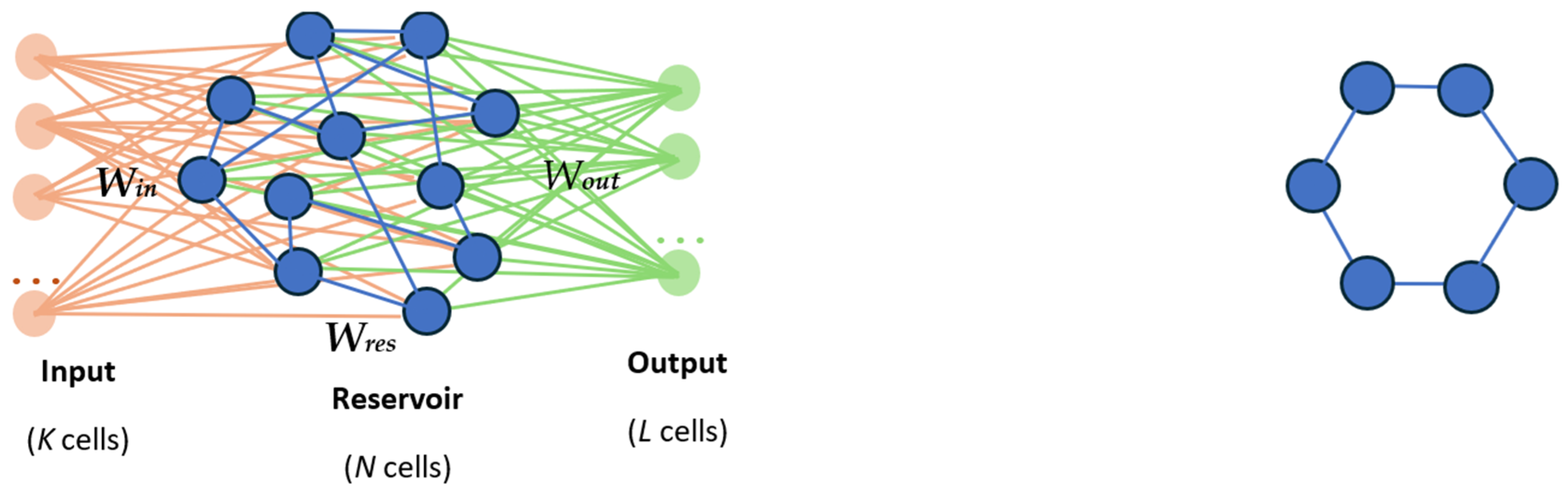
Reservoir computing (RC) has gained recognition as an efficient method for handling sequential and time-dependent data, especially in cases where traditional recurrent neural networks (RNNs) become too complicated or computationally heavy to train. Conventional RNNs require training of all internal weights of the couplings among individual cells (nodes) of the hidden layer, together with the weights coupling the input to the hidden layer and the weights of the coupling between the hidden layer and the output. This training often relies on resource-intensive algorithms such as Backpropagation Through Time (BPTT) [1]. RC uses a unique structure, illustrated in Figure 1, that drastically reduces training complexity. It consists of a hidden layer containing N hidden units (the reservoir) that are randomly and sparsely connected, with connection weights Wres selected randomly in the interval [−1, 1]. These weights remain fixed without training. The input layer consists of K cells, depending on the structure of the input data, each connected to all reservoir units via weights Win ( K × N matrix), which are also initialized randomly in the range [−1, 1] and remain fixed. The only weights that are optimized during training are those linking the reservoir to the output layer, Wout, sized L × N .
This approach reduces both computational cost and training time, making RC practical for software and hardware implementations. On the other hand, this design shows surprisingly good performance that, for most tasks, is comparable to, or better than, other approaches like LSTMs or CNNs, which include more complicated ML methods. The main architectures under RC are Echo State Networks (ESNs) [2], Liquid State Machines (LSMs) [3], and Time Delay Reservoirs (TDRs) [4]. Of these, ESNs, first proposed by Jaeger in 2001 [2], are essentially a kind of RNN notable for their straightforward design and efficiency. Their success relies on the Echo State Property (ESP), which ensures that the network’s internal state reliably distinguishes features and correlations among different input signals, independent of the internal variables’ initial conditions. This means that the ESN internal state correctly “echoes” the state of the input, thereby maintaining consistent and reliable outputs. Interestingly, studies show, both in time-series forecasting and classification tasks, that even a randomly connected high-dimensional dynamical system can approximate the dynamics of any other system of lower dimensionality, if provided with enough data. In other words, ESNs exploit this by projecting input signals into a high-dimensional non-linear space within the reservoir to encode input features over time. Then, one needs to train only the weights from the reservoir-to-output layer connections, to train “the observer” rather than the system itself. This allows ESNs to perform excellently in applications such as time-series forecasting, pattern recognition, classification, and system modeling tasks [5].
Consider a discrete input sequence consisting of vectors u n of dimension K, for each time step n, along with a corresponding target output sequence y n t a r g e t of dimension L. At every step, the ESN updates its internal state vector x n of dimension N, whose components are the values x n i of the internal variables of reservoir cell i at time step n, according to the master equation:
x n + 1 = ( 1 α ) x n + α   t a n h ( G ( θ W i n · u n + 1 + W r e s · x n ) + b ) ,
where α represents the leaking rate, which controls how much the next reservoir state depends on the previous state, tanh(…) is the (sigmoidal) activation function of the cells, G, b are fixed constants that define the gain and bias of the activation function, and θ is a constant parameter by which the input vector is scaled before entering the activation function. Among the system’s hyperparameters, α and θ together with the spectral radius ρ of the fixed weight matrix of the reservoir W r e s are the most critical and typically need to be tuned for each specific task. Finally, the output signal of the reservoir is determined as a linear combination of state vectors x n :
y n r e s = W o u t · x n .
It is worth noting that variations of Equations (1) and (2) have appeared in applications such as, for example, the inclusion of feedback terms in the activation function, or a non-linear function determining the output of the reservoir from the linear combination of the reservoir states. However, (1) and (2) are sufficient for the application in the present work. The elements of the output weight matrix W o u t can be determined very efficiently using a straightforward solution of an overdetermined linear algebraic system of equations:
W o u t = Y t a r g e t · X ,
where Y t a r g e t contains the target output vectors y n t a r g e t as its columns, and X is the pseudo-inverse of the matrix whose columns are all the corresponding reservoir states x n . Equation (3) represents a linear least-squares problem, where the elements of W o u t ( L × N ) are chosen to minimize the total difference between the reservoir outputs y n r e s and the target outputs y n t a r g e t . This method is extremely fast, requires only a single step, and always converges, unlike the complicated and multi-step BPTT training algorithm by which normal ANNs are usually trained.
A crucial part of implementing an ESN is tuning the key hyperparameters ρ, α, and θ, which determine the responsiveness, memory capacity, and non-linearity of the reservoir [5]. The connectivity (density of non-zero weight connections among reservoir cells) may also influence network dynamics and performance. However, in most applications in the past, it has been shown that even very sparsely connected reservoirs perform well; in fact, optimum performance is most often achieved with sparse rather than fully connected reservoirs. The gain G and bias b of the activation function may also be optimized, and, of course, alternative sigmoidal activation functions can be used in place of tanh(). However, among all factors, the size of the reservoir, defined by the number of internal cells N, is the most critical determinant of performance. N must also be optimized depending on the specific problem and the available training data. In general, the more cells the better, since larger reservoirs improve ESN’s ability to represent complex dynamics and capture internal correlations. A natural upper limit to N is obtained when overfitting sets in, a common risk in all ANNs, i.e., when the ESN specializes in fitting training data almost perfectly but then loses the ability to perform well in unseen data.
In terms of training time and computational resources, increasing the number of hidden cells N of the ESN reservoir (unlike in other RNNs) has minimal impact, since ESN’s training is extremely fast and scales with N2, which is a major advantage over conventional RNNs. However, care must be taken to avoid overfitting, particularly when the training dataset is small. The reservoir’s geometry and topology can also be adjusted. In the originally proposed version of ESN, the reservoir is composed of a single layer with randomly connected cells. However, deep or multi-layer reservoirs and alternative connection schemes have been proposed [6]. Our own version of ESN (Multi-ESN) allows multi-layered reservoirs of various configurations. Because there is no analytical solution for selecting the optimum values of the hyperparameters, tuning usually requires empirical testing across multiple configurations. In practice, however, and for most applications, optimizing the basic parameters ρ, α, and θ and the size N of a random reservoir is often sufficient to achieve excellent performance, while factors such as geometry, connectivity, and the other mentioned parameters are generally secondary. Random initialization of the reservoir further motivates performing multiple trials from different starting points to assess stability, robustness, and maximize performance [5]. Despite these complexities, the total training time required for an ESN (including hyperparameter optimization) is drastically less than that for conventional RNNs. Overall, the computational elegance, simplicity, and capacity of ESNs for modeling complex temporal dependencies have made them an increasingly popular tool in fields ranging from speech and signal processing to biomedical diagnostics, including promising applications in ECG-based health prediction and classification tasks.
For biomedical time-series classification, in particular, ESNs have been widely studied due to their efficient temporal modeling, low training complexity, and robustness to input signal noise. More specifically, in ECG analysis, ESN-based approaches have demonstrated strong performance in ventricular heartbeat classification, achieving accuracies above 95% on the MIT-BIH arrhythmia dataset and enabling real-time monitoring [7,8]. Patient-adaptable reservoir computing models further improve classification performance through adaptive readout strategies [9]. More recently, a normalized ESN architecture (called NESN) has been proposed to enhance stability and robustness to non-stationary and noisy ECG signals, leading to improved abnormal pattern detection [10]. Beyond ECG, ESNs have also been successfully applied to EEG classification tasks, including mental-task brain–computer interface systems [11] and wrist and grip movement decoding, demonstrating accurate motor-related EEG classification with low computational complexity [12]. Studies on reservoir dynamics have also shown that performance and internal representations are affected by updates to internal parameters such as gain and bias, with improved separation of states and prediction accuracy occurring near critical dynamic regimes [13]. The robustness of ESNs under noisy conditions has been explicitly investigated, with stable performance reported in noisy classification and speech recognition tasks [14,15] as well as time-series classification under Gaussian noise interference [16]. In all the above-mentioned works, the goal was to maximize ESN recognition accuracy and uniformity across classes, whereas noise was considered only for the input data.
In the present work, we first evaluate the performance of single-layer and multi-layer ESN with deep architecture in the classification of individual ECG heartbeats, with five classification categories. We used supervised training of the ESN without combining it with other AI systems or ML methods and without any input signal pre-processing, such as denoising or feature extraction, just signal normalization. We compare the performance of (i) a “ring” reservoir, which has the sparsest possible cell connectivity, as all cells form a ring structure and each cell is connected to only two of its neighbor cells, and (ii) a normal randomly connected reservoir, which is more densely connected. Moreover, we investigate how introducing noise in the dynamics of the internal variables of the reservoir (rather than the input data) influences ESN performance. We also investigate how ESN performance is influenced if random variability is imposed in the gain and bias parameters of the activation function in each cell of the reservoir. The latter questions are of importance, especially considering possible analog implementations of the ESN with technologies other than CMOS, which is the main concept behind reservoir computing. In such implementations, robustness of ESN performance under noisy conditions within the reservoir hardware and/or non-identical reservoir cells is crucial. Also, it is important to demonstrate how reservoirs with the sparsest possible connectivity (ring reservoirs) perform in ECG pulse recognition tasks because these reservoirs would have lower manufacturing costs. Finally, we compare the performance of our ESN results with those reported in previous studies using other ANN-based models, both in terms of recognition accuracy and in terms of training times and computing resources.

2. Methodology

2.1. Description of ECG Dataset

The ECG heartbeat classification experiments were conducted using the PhysioNet MIT-BIH arrhythmia database [17], specifically a version that was pre-processed by Kachuee et al. [18]. The MIT-BIH arrhythmia database is a widely accepted benchmark for evaluating classification algorithms using one-dimensional signals. It contains 48 half-hour electrocardiogram (ECG) recordings collected from 47 different individuals, which were randomly selected from a larger set of 4000 full-day ECG recordings. The selection strategy ensured the inclusion of both frequently occurring arrhythmias and clinically important but relatively rare arrhythmia types that might be absent from a smaller dataset. All ECG signals were digitized at a sampling rate of 360 samples per second. In addition, each recording was independently reviewed and annotated by at least two cardiologists to ensure the reliability of the pulse classifications. The pre-processing pipeline described by Kachuee et al. provides a detailed description of how the ECG signals were processed, including heartbeat segmentation and extraction procedures. Experts’ annotations were classified into five categories, according to the Association for the Advancement of Medical Instrumentation (AAMI) EC57 standard [19], as follows: Category 0 (N): Normal beat; Category 1 (S) Supra-ventricular ectopic beat; Category 2 (V): Ventricular ectopic beat; Category 3 (F): Fusion beat; Category 4 (Q): (Q) Unknown beat. In the next step, the authors of ref. [18] employed a deep convolutional neural network (CNN) with residual connections to classify the ECG heartbeats, achieving a peak accuracy of 93.4%. Finally, after the processing of the ECGs, a labeled dataset of individual heartbeats was produced with class labels 0–4 depending on the category to which each belongs, with 87,554 heartbeats for training and 21,892 heartbeats for testing. These files are publicly available [20].

2.2. ESN Setup

The experiments in this work were carried out using a custom MATLAB-based software tool named Multi-ESN that was run in MATLAB v2024b for Microsoft Windows 11 64bit environment on an Intel i5-1235U @ 1.3 GHz/CPU/36GB DDR4 laptop PC. developed by the first author of this paper. This tool is based upon Deep-ESN code available publicly by Gallicchio et al. [6]. Multi-ESN enables the construction of multi-layer reservoir computing architectures as well as a variety of geometries per layer, like the ring geometry shown in Figure 1. Multi-ESN can be used for both time-series forecasting and classification problems.

2.3. ESN Input Dataset: Description and Pre-Processing

The ECG heartbeat dataset used in this study contained 87,554 samples. Each sample is a piece of an ECG signal representing a single heartbeat. All samples have 187 datapoints and are of the same time duration. To form the input vector time-series for the ESN, each sample signal was stored as a column vector of 187 elements.

2.3.1. Dataset Balancing

The distribution of samples across the five heartbeat classes was highly imbalanced: Class 0: 72,471 samples, Class 1: 2223 samples, Class 2: 5788 samples, Class 3: 641 samples, and Class 4: 6431 samples. To facilitate the procedure, the dataset was split into three subsets: 80% for training, 10% for validation, and the remaining 10% for testing. Samples were randomly shuffled to ensure a uniform representation of each category across all three subsets. Preliminary experiments indicated that improving the class distribution homogeneity would likely benefit both the training process and the overall performance of the reservoir. This was particularly important given the extreme imbalance in the training set, where Class 0 had nearly 58,000 samples, whereas Class 3 had only 520. The effect of a severely imbalanced training dataset being fed into the ESN, just as in any ANN-based ML classification system, is an analogous imbalance in its classification ability per class: the ESN is expected to perform excellently in over-represented classes while poorly in under-represented ones; the greater the imbalance in the dataset, the greater the inhomogeneity in performance across classes. This happens because the ANN loss function weighs all samples uniformly, and thus, the ANN is trained based on the ESN’s average performance across all classes, not per individual class. To confront this issue, we balanced the dataset by simple sample replication for the minority classes. Specifically, the dataset was modified so that each one of the five classes contains 20,000 heartbeats. For classes initially containing more than 20,000 samples, a subset of 20,000 heartbeats was randomly selected. For classes with fewer than 20,000 samples, a randomly selected subset of as many distinct samples as possible was replicated as necessary to reach the desired number. As a result, the final input dataset used for training and testing the reservoir consisted of 100,000 heartbeat signals in total, evenly distributed across all five categories, randomly permuted. The random shuffling and especially the “balancing” of the training set are crucial for achieving comparable recognition accuracy across all classes.
At this point, we should mention that several other methods have appeared in the literature for balancing unbalanced datasets regardless of the AI method or classification task. The most important are as follows: Data augmentation, which mitigates imbalance by generating additional, label-preserving transformed samples. This increases the diversity of minority classes without the need to collect new data [21]. SMOTE (Synthetic Minority Over-sampling Technique) balances classes by creating new minority instances through interpolation between a sample and its nearest neighbors instead of simple replication [22]. Adaptive sampling strategies dynamically concentrate synthetic generation or sampling effort on harder-to-learn minority examples rather than oversampling uniformly [23]. Finally, cost-sensitive learning is a technique that addresses class imbalance by assigning higher misclassification costs (or loss weights) to minority classes, so that the optimizer gives priority to reducing their errors [24]. All the above methods are more “sophisticated” alternatives than the simplest choice, sample replication for the minority classes. A simple replication strategy may pose increased risk for overfitting and generalization relative to the more sophisticated methods. So why did we choose a simple sample replication method? The simple answer is that, in retrospect, it worked very well, judging by the excellent recognition rate across all classes. However, we initially chose to stick with this choice mainly for two reasons: First and foremost, because we intend to utilize the simplest training and operational protocol possible for our ESN system without significantly compromising performance, keeping in mind that the long-term goal is a cost-effective implementation with analog hardware (see also our discussion in the next paragraph). For this reason, the simplest balancing procedure possible is the obvious choice. Secondly, we argue that, for our task and dataset, the risks for generalization are not expected to be noticeably reduced by any one of the more sophisticated balancing methods. Firstly, because the training dataset is already very large, containing, in absolute numbers, many samples even for the minority classes. (The most severely under-represented class already has 641 distinct samples.) In fact, it is not even guaranteed that the most sophisticated methods would perform better, while they might as well perform worse. For example, SMOTE, while producing synthetic samples by interpolating between “nearest neighbors”, may generate unrealistic samples that lack key features of the originals and end up “confusing” the ESN. By simple replication, we ensure that the ESN is always looking at real samples from each class and with the same frequency. Of course, a thorough case study utilizing all balancing methods and comparing results would reveal which method performs best; however, this comparison is beyond the scope of the present work and is left for the future.

2.3.2. Signal Pre-Processing

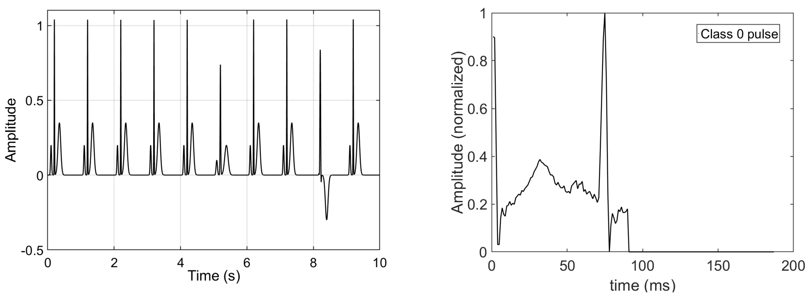
No extra pre-processing was applied to the raw ECG pulse signals as obtained from the PhysioNet MIT-BIH arrhythmia database. In this database, the amplitude of all the raw signals is already normalized in the interval [0, 1], as seen in Figure 2, apparently by min-max scaling. This is the standard and necessary procedure to bring the scale of the input within the activation range of the hyperbolic tangent function used as activation function for all neuronal nodes of the reservoir. We did not perform any denoising of the signals. We did not apply any feature extraction techniques, such as, for example, the number and position of signal extrema, their relevant temporal spacings, etc. We used the raw (normalized) signals exactly as obtained from the database. Our purpose is to test the ability of the ESN to learn by “brute-force” the relative correlations existing in the raw signals well enough so that it correctly distinguishes among the different pulse classes. In general, it is known that training any RNN with denoised data and especially providing low-dimensional auxiliary information about the input signals may significantly enhance its performance while reducing the required hidden layer size (number of neuronal cells). However, this practice merely shifts part of the weight from the RNN to the system that must implement pre-processing steps. The same argument given in the previous paragraph about the choice of balancing method is also given here; the long-term goal of reservoir computing, in general, is to realize cost/resource-effective, analog hardware implementations of the reservoir (the ESN in our case) that perform equivalently to digitally implemented AI systems. This means that one should seek to simplify their training and operation protocols as much as possible; ideally, both should be carried out in one step and with a single component.

2.4. ESN Target and Output Signal Post-Processing

In the original dataset [18], each heartbeat was labeled using an integer value between 0 and 4 corresponding to its category. The target set was shuffled in the same order as the input data to maintain input-target alignment. Since reservoir output signals are always continuous numbers, an extra processing step is required to map the output signal to discrete class labels. Using consecutive integers 0,1,2,3,4 as class labels and a “floor” function for mapping the continuous ESN output y to one of the integers is one way to do it. However, this strategy introduces an undesirable bias, as it forces the network to produce progressively larger output magnitudes for classes labeled with higher integer values. In order to eliminate this bias we used a one-hot encoding format labeling each category as a five-dimensional binary vector, as follows: category 0 → [1 0 0 0 0], class 1 → [0 1 0 0 0], class 2 → [0 0 1 0 0], class 3 → [0 0 0 1 0], and class 4 → [0 0 0 0 1]. Accordingly, the reservoir output must now be a five-dimensional continuous signal (y0, y1, y2, y3, y4). The mapping of this continuous-valued vector to one of the above binary strings is then completed simply by a “winner-takes-it-all” strategy, i.e., the component yi with the highest absolute value is the decided class.

2.5. ESN Optimization

The baseline configuration, hereafter referred to as the default reservoir (DF), consisted of a single-layer architecture with a total of 300 reservoir nodes, evenly distributed across layers (100 nodes per layer). Each layer had a ring topology, meaning that only two non-zero weight connections were realized between each node and its two immediate neighbors on the ring, resulting in minimal intra-layer connectivity. Typically, the number of layers is not considered a hyperparameter, as the reservoir in standard ESNs usually consists of a single layer of recurrent nodes. We initially focused on optimizing the basic parameters α and the spectral radius ρ simultaneously. The leaking rate α ranged in the interval [0.5, 1] and the spectral radius ρ within the range [0.2, 1.2], also with a step size of 0.1. The optimization’s attention then shifted to parameters such as the input scaling θ, the gain G, and bias b, the parameters that directly affect the pre-activation that passes into the activation function. These three were tuned simultaneously with the range for input scaling [1, 4] with step size 1, for gain [0.5, 2.5] with step size 0.5, and for bias [−1.5, 1.5] with step size 0.75. The optimal values obtained were fixed before proceeding to subsequent optimization stages.
The next step explored the impact of reservoir size and geometry. First, we varied the total number of nodes in the range of 150 to 4800 using the ring geometry. Alternatively, we tried a random geometry (with random connectivity in the reservoir and non-zero weight connections). Finally, a deep architecture with randomly connected layers arranged in series was tested, where only the first layer was connected to the input layer and only the final layer was connected to the output.

3. Results

3.1. Effect of Input Balancing and Each Step of Hyper-Parameter Optimization on ESN Performance

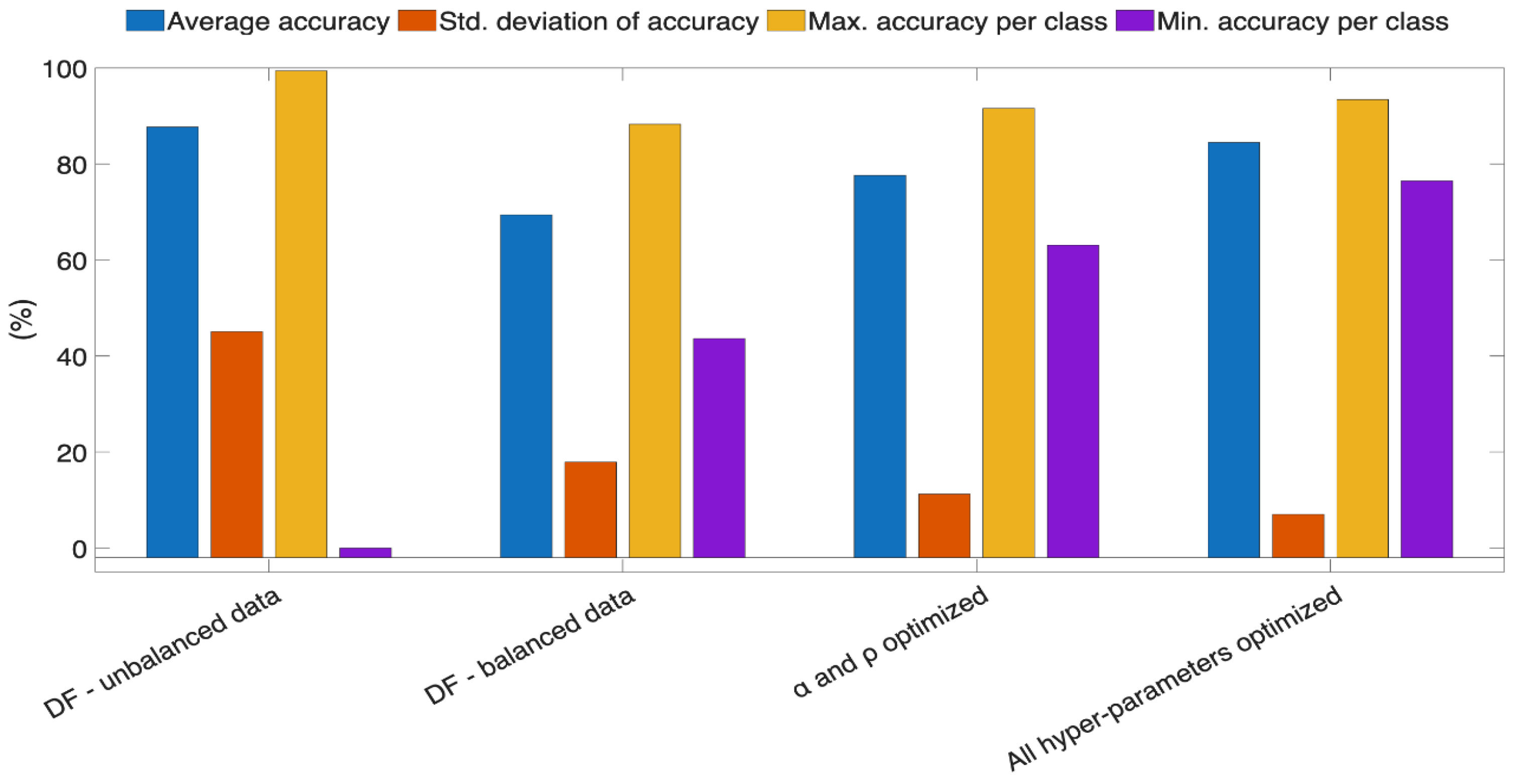
During the first stage of hyperparameter tuning, using the 300-node reservoirs, for the leaking rate and spectral radius, we found optimal values α = 1 and ρ = 0.2, respectively. This optimization was performed using both balanced and unbalanced datasets, yielding identical optimal values in both cases. As expected, tuning the leaking rate is not necessary for this classification task, since the ECG samples are independent of one another. Thus, the ESN does not require temporal memory. For the optimal values of these parameters, there is a notable difference in the % accuracy between balanced and unbalanced data, as shown in Figure 3. The ESN that was trained with unbalanced data showed an almost perfect accuracy in classifying category 0 pulses (99.4%), which are the most represented in the dataset, but only 0.0% in classifying pulses of category 3 (the most severely under-represented). Average % accuracy across classes appears high (87.7%), but this result was misleading due to the extremely high standard deviation of the recognition accuracies for each class (45.1%). This indicates that signals belonging to minority classes were effectively ignored in the learning process. After balancing the input dataset, even without optimized hyperparameters, the overall accuracy decreased to 69.4%, but performance across categories became significantly more uniform. The per-class accuracy standard deviation dropped to 17.9%, while the accuracy for the least-recognized class improved from 0.0% to 43.6%. Subsequent optimization of ρ and input scaling θ increased the overall accuracy to 77.6%, reduced the standard deviation to 11.2%, and raised the accuracy of the least-recognized class to 63.1%. Finally, joint optimization of θ, G, and b for the 300-node ESN yielded the optimal values (θ = 4, G = 1, and b = 1.5), further improving the average accuracy, standard deviation, and lowest accuracy per-class to 84.5%, 7.0%, and 76.5%, respectively.
Notably, training a 300-node ESN required approximately 9 s per ESN on an Intel i5-1235U @ 1.3 GHz CPU using the MATLAB implementation of the Multi-ESN framework. In Table 1, we summarize the optimal values of the basic ESN hyperparameters.

3.2. Multi-ESN Performance vs. Reservoir Size and Reservoir Geometry

After optimizing the fundamental reservoir hyperparameters using relatively small networks, with extremely fast training sessions, these parameters were fixed for all subsequent experiments. We then examined the influence of reservoir size (number of hidden cells) and cell connectivity on the overall performance of the ESN.
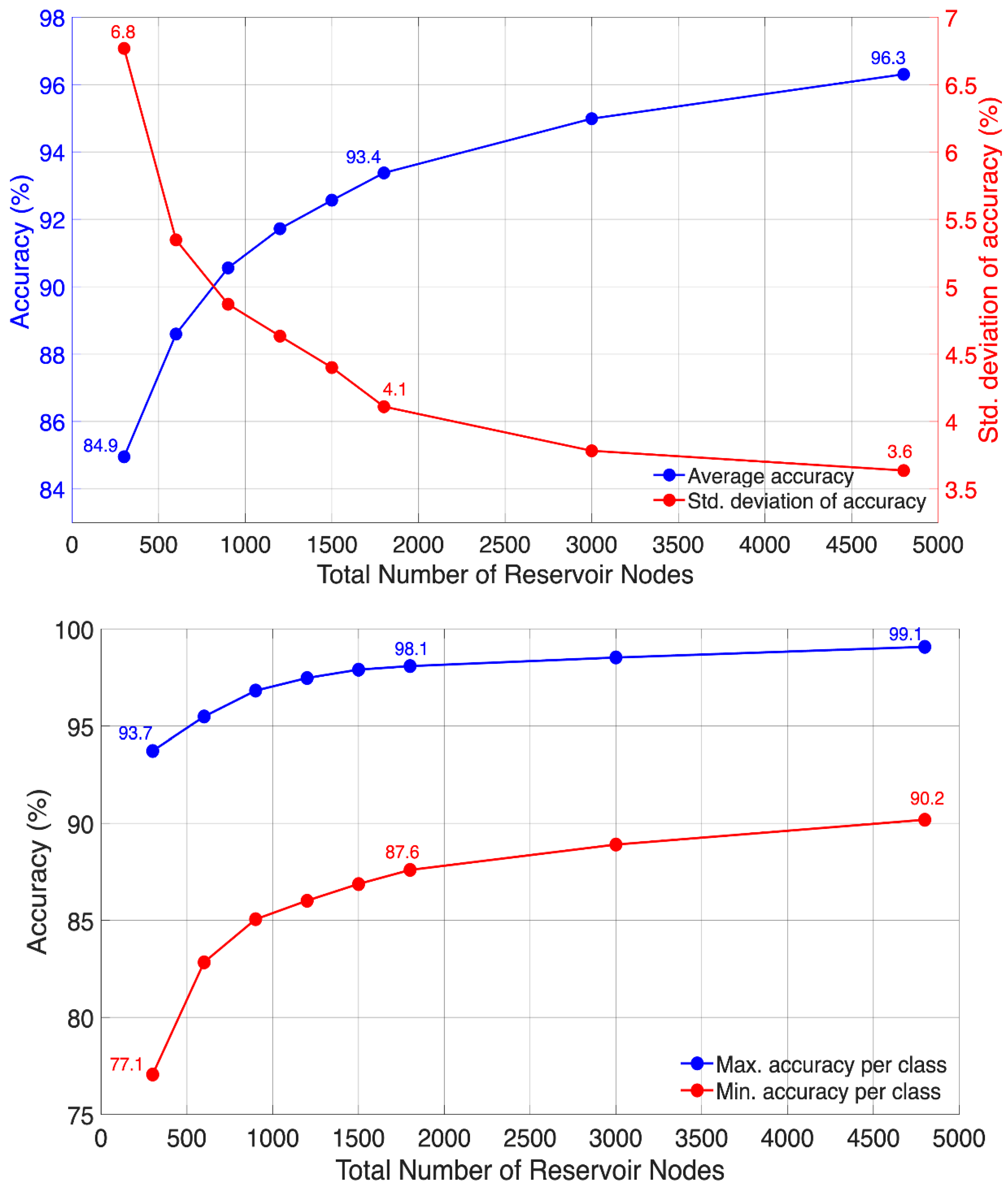
Figure 4 depicts the performance of the reservoir as a function of reservoir size, confirming that an increase in the number of nodes generally leads to consistent improvement in performance. In particular, the highest overall accuracy of 96.3% was achieved using the largest reservoir tested, which contained 4800 nodes. However, already with a 1800-node ESN, the % accuracy, on the overall and per-class, is almost identical to the results of ref. [18]. Our 3000-node ESN already surpasses the average accuracy of the highest performing study referenced in Table II of ref. [18].
In Table 2, we show a comparison between the accuracy achieved for various ESNs of the present study relative to other similar studies for ECG heartbeat classification involving other ML methods, all using the same ECG pulse database as ours.
In Table 3, we compare the performance of an ESN with a reservoir of N = 1200 nodes and ring geometry and an ESN of N = 1200 nodes and random connectivity with 20% of intra-reservoir connections having non-zero weights (density = 0.2). We also show results for a deep ESN architecture in which the 1200 nodes of the reservoir are distributed in three layers of 400 nodes each, while only the first layer is connected to the input cells and only the last layer is connected to the output cells.
Reservoir performance was essentially unaffected by intra-reservoir connectivity when the same optimized hyperparameter values were used. Configurations with very different intra-layer sparsity, such as the ring-based and random geometries with increased density of non-zero connections, achieved nearly identical classification accuracy. This is an important result for potential analog realizations of ESNs, where fewer connections reduce structural complexity and manufacturing cost.
A deep architecture was not beneficial at all. While deep architectures often improve performance in other ANN models, we did not observe this for ESNs. Shallow reservoirs with optimized geometries reach accuracy levels close to 92%, whereas the deep architecture dropped to 72%. Depth appears to add unnecessary complexity without improving performance in RC-based models. In RC, reservoir and input weights are fixed, and only the readout is trained. The reservoir acts as a high-dimensional non-linear dynamical system that remains fixed during training while driven by a lower-dimensional input signal. As such, it projects the input into an orbit in a much higher-dimensional phase space. Because internal weights are not optimized, it is important to connect every reservoir cell to the output layer to exploit the reservoir’s full predictive power. Likewise, each input component should ideally connect to every reservoir cell to maximize the ways the input can drive the reservoir’s internal state. Deep architectures do not fulfill these conditions: the input signal drives only the cells of the first layer, and the ESN output signal depends only on the cells of the last layer. This reduces the number of combinations by which the input signal is weighted before being fed to the reservoir as well as the number of trainable readout weights, rendering intermediate layers largely unhelpful. In summary, ESN performance benefits most from large, shallow reservoirs with full input-to-reservoir and reservoir-to-output connectivity; reservoir geometry and internal sparsity are secondary.

3.3. Effect of Noisy Reservoirs and Random Variability in Reservoir Cell Activation Functions on ESN Performance

In this section we present the results for the experiments in which we have introduced noise into the reservoir dynamics. We did this by adding a Gaussian noise term in the recursion equation that updates the values of the reservoir state variables x n + 1 as follows:
x n + 1 = ( 1 α ) x n ( 1 + A   ξ n ) + α   t a n h ( G ( θ W i n · u n + 1 + W r e s · x n ( 1 + A   ξ n ) ) + b ) ,
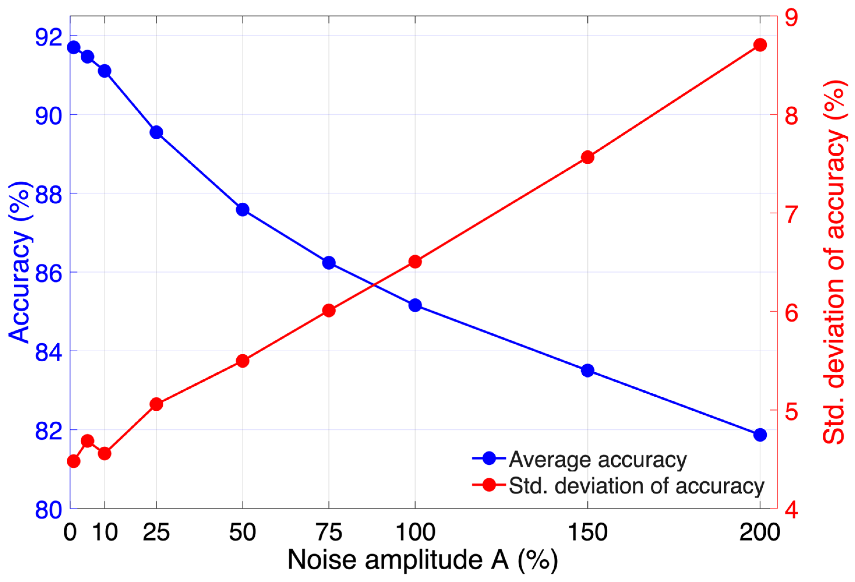
where ξ n is a vector of dimension N whose components are random variables distributed according to the normal distribution. A is a constant parameter that determines the amplitude of the noise term relative to x n . As a basis, we used the optimized ESN with 1200 nodes, evaluating its performance for noise amplitudes A = 1%, 5%, 10%, 25%, 50%, 75%, 100%, 150%, and 200%. The results are shown in Figure 5.
We see that, as the noise level increases, the performance of the reservoir decreases, as expected, however, at a surprisingly slow rate. Overall accuracy dropped from ~92% to only ~82% at the highest noise level of 200%, while the standard deviation of accuracy across classes increases from ~4.7 to 8.7%. In the context of this study, an ESN model is considered reliable if its performance degrades by no more than 10% when subjected to noise of up to 25% signal-to-noise ratio relative to the amplitude of reservoir state variables x n . This threshold is based on empirical observations and practical robustness considerations and is supported in the literature. In our case, the overall accuracy reduction at 25% noise-to-signal ratio is only about 2.3%; thus, the ESN model satisfies this reliability criterion and proves very robust under the presence of noise.
Next, we examined the effect of adding random variability at the activation function of each cell of the reservoir by introducing small random fluctuations in the gain and bias of the non-linear term of Equation (3). We did this by letting the trainable but constant for all reservoir cells parameters G and b vary by assigning different values to them for each cell i as follows:
G i = G + N ( 0 , σ G ) ,   b i = b + N ( 0 , σ b )
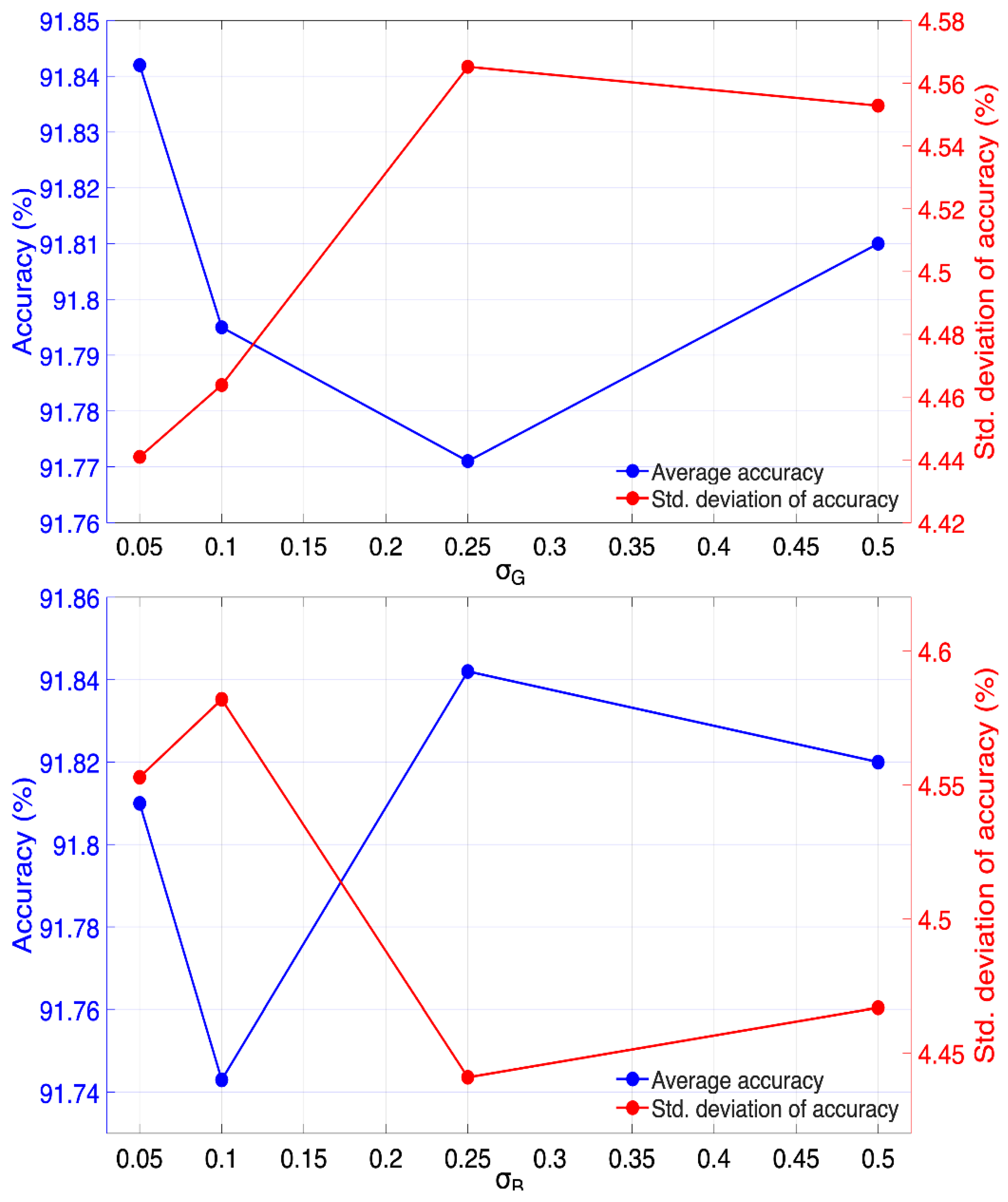
where N ( 0 , σ G ) and N ( 0 , σ b ) are the normal distributions with mean 0 and standard deviation σ G and σ b , respectively. The latter parameters measure the degree of random variability across cell activation functions. These fluctuations can cause the activation function to produce different outputs, even when the weights of the reservoir layer remain constant. Then, we trained a corresponding ESN of 1200 nodes by varying the values of σ G and σ b while optimizing G and b together with all the usual hyperparameters as before. The variation in ESN performance with cell variability level is shown in Figure 6. Clearly, introducing random variability in the gain and bias parameters of the activation function does not practically affect the reservoir’s performance at all. The ESN’s accuracy remains between about 91.74% and 91.84%, with only a small standard deviation, even when both σ G and σ b are varied simultaneously.

4. Discussion and Conclusions

In this study, an Echo State Network was applied to a five-class ECG heartbeat classification problem with a training set that is strongly unbalanced in terms of annotated samples per category. We demonstrated that balancing the training data by replicating samples from under-represented categories so that all categories are equally represented in the training set substantially improves classification consistency across all heartbeat categories. We also showed that the overall % accuracy and its uniformity across classes are substantially affected by the size of the reservoir. The highest overall accuracy achieved was 96.3%. The minimum accuracy per class (for the severely under-represented class) was 90.2% with an ESN of 4800 nodes. This is higher than at least four prior studies employing more complex machine learning approaches. Already, with a smaller ESN of 1800 nodes, we achieved an overall accuracy of 93.4% with the lowest accuracy per class, 87.6%, which reached the same level as previous studies. Equally significant is the computational efficiency of the proposed approach. Training times for ESNs were found to be only a fraction of those required by alternative methods based on RNNs or CNNs, which allows the training of even the largest ESNs to be carried out with much lower computational resources than those required for training more traditional methods (CPUs instead of GPUs).
Secondly, our results indicated that ESNs with reservoirs having the “ring” architecture, the most economical one in terms of number of connections, perform equally well in the ECG classification task compared to denser random architectures. This and important result for hardware implementations where saving on resources in manufacturing is an issue. Thirdly, we found that deep architectures, in which the reservoir is divided into distinct layers sequentially connected to each other, while only the first layer is connected to input and only the last to output, are not at all beneficial to ESN performance. The best architecture is clearly when all input and output cells are connected to every reservoir cell and thus the reservoir is a single layer.
Finally, it was found that adding random variability to the activation function gain and bias parameters, essentially creating a reservoir with diverse neuronal cells, hardly has any impact on the overall performance of the ESN. Moreover, we showed that, after adding Gaussian noise to the dynamics of the state variables of the reservoir cells, it still maintains exceptionally good performance even for very high noise levels. Average accuracy is only slightly (2.3%) affected by added noise for a noise-to-signal ratio of up to 25%. This is particularly important for possible physical implementations of RCs with analog hardware. Flexible and reliable analog implementations can be considered as the holy grail in reservoir computing in general. Analog implementations of RCs and ESNs, besides being much faster and simpler in training, also avoid some disadvantages of digital computing, such as high cost and high-power consumption. The latter are undesirable in certain applications, especially in the Internet of Things and edge computing. On the other hand, analog implementations of ESNs face some challenges. First, they usually require (as also seen in the present study) very large-sized reservoirs with several hundreds or even thousands of nodes to perform equivalently to conventional RNNs, especially in time series classification tasks where each sample has many datapoints. This poses difficulties in manufacturing and operation. A second challenge in these analog implementations often revolves around internal noise (e.g., thermal noise or process variation) and non-ideal device behavior, which can degrade the useful signal. It is the second challenge that we tried to address in the present study by showing that even noisy and highly variable reservoirs can perform well, at least in a time-series classification task. Apparently, the characteristic features that distinguish between time-series (signals) belonging to different classes are easily learned by ESNs with large enough reservoirs, while the differences between these features are not severely obscured even with high levels of noise and variability.

Author Contributions

Conceptualization, I.P.A.; Data curation, A.N.T.; Methodology, I.P.A. and A.N.T.; Software, I.P.A.; Validation, C.K.V., A.D.T. and K.G.K.; Formal analysis, I.P.A. and C.K.V.; Writing—original draft, I.P.A. and A.N.T.; Writing—review & editing, I.P.A., A.N.T., C.K.V., K.G.K. and H.E.N.; Visualization, A.N.T. and I.P.A.; Supervision, I.P.A., C.K.V., A.D.T. and H.E.N.; Project administration, C.K.V. All authors have read and agreed to the published version of the manuscript.

Funding

This research received no external funding.

Data Availability Statement

The data presented in this study are available upon request.

Conflicts of Interest

The authors declare no conflict of interest.

References

  1. Schmidt Robin, M. Recurrent neural networks (RNNs): A gentle introduction and overview. arXiv 2019, arXiv:1912.05911. [Google Scholar] [CrossRef]
  2. Jaeger, H. The Echo State Approach to Analysing and Training Recurrent Neural Networks—With an Erratum Note; GMD Technical Report; German National Research Center for Information Technology: Bonn, Germany, 2001; Volume 148, p. 13. [Google Scholar]
  3. Maass, W.; Natschläger, T.; Markram, H. Real-time computing without stable states: A new framework for neural computation based on perturbations. Neural Comput. 2002, 14, 2531–2560. [Google Scholar] [CrossRef] [PubMed]
  4. Appeltant, L.; Soriano, C.M.; Van der Sande, G.; Danckaert, J.; Massar, S.; Dambre, J.; Schrauwen, B.; Mirasso, C.R.; Fischer, I. Information processing using a single dynamical node as complex system. Nat. Commun. 2011, 2, 468. [Google Scholar] [CrossRef] [PubMed]
  5. Lukoševičius, M. A Practical Guide to Applying Echo State Networks. In Neural Networks: Tricks of the Trade; Montavon, G., Orr, G.B., Müller, K.R., Eds.; Lecture Notes in Computer Science; Springer: Berlin/Heidelberg, Germany, 2012; Volume 7700. [Google Scholar]
  6. Gallicchio, C.; Micheli, A.; Pedrelli, L. Deep reservoir computing: A critical experimental analysis. Neurocomputing 2017, 268, 87–99. [Google Scholar] [CrossRef]
  7. Mastoi, Q.U.A.; Wah, T.Y.; Raj, R.G. Reservoir computing based echo state networks for ventricular heartbeat classification. Appl. Sci. 2019, 9, 702. [Google Scholar] [CrossRef]
  8. Ortín, S.; Soriano, M.C.; Alfaras, M.; Mirasso, C.R. Automated real-time method for ventricular heartbeat classification using reservoir computing. Comput. Methods Programs Biomed. 2019, 169, 1–8. [Google Scholar] [CrossRef] [PubMed]
  9. Hadaeghi, F. Reservoir computing models for patient-adaptable ECG monitoring. arXiv 2019, arXiv:1907.09504. Available online: https://arxiv.org/abs/1907.09504 (accessed on 1 December 2025).
  10. Wang, S.; Ding, C.; Wang, Z.; Shen, L. Using normalized echo state network to detect abnormal ECG patterns. Int. J. Imaging Syst. Technol. 2024, 34, e22940. [Google Scholar] [CrossRef]
  11. Forney, E.M.; Anderson, C.W.; Gavin, W.J.; Davies, P.L.; Roll, M.C.; Taylor, B.K. Echo State Networks for Modeling and Classification of EEG Signals in Mental-Task Brain–Computer Interfaces; Technical Report CS-15-102; Colorado State University: Fort Collins, CO, USA, 2015. [Google Scholar]
  12. Khan, Z.H.; Hussain, N.; Tiwana, M.I. Classification of EEG signals for wrist and grip movements using echo state network. Biomed. Res. 2017, 28, 1095–1102. [Google Scholar]
  13. Morales, G.B.; Mirasso, C.R.; Soriano, M.C. Unveiling the role of plasticity rules in reservoir computing. arXiv 2021. [Google Scholar] [CrossRef]
  14. Prater, S. Comparison of echo state network output layer classification methods on noisy data. arXiv 2017, arXiv:1703.04496. [Google Scholar] [CrossRef]
  15. Skowronski, M.D.; Harris, J.G. Noise-robust automatic speech recognition using a predictive echo state network. IEEE Trans. Audio Speech Lang. Process. 2007, 15, 1724–1730. [Google Scholar] [CrossRef]
  16. Xia, L.; Tang, J.; Li, G.; Fu, J.; Duan, S.; Wang, L. Time series classification based on forward echo state convolution network. Neural Process. Lett. 2024, 56, 173. [Google Scholar] [CrossRef]
  17. Moody, G.B.; Mark, R.G. The impact of the MIT-BIH Arrhythmia Database. IEEE Eng. Med. Biol. Mag. 2001, 20, 45–50. [Google Scholar] [CrossRef] [PubMed]
  18. Kachuee, M.; Fazeli, S.; Sarrafzadeh, M. ECG heartbeat classification: A deep transferable representation. In 2018 IEEE International Conference on Healthcare Informatics (ICHI); IEEE: New York, NY, USA, 2018; pp. 443–444. [Google Scholar]
  19. ANSI/AAMI EC57:1998(R)2008; Testing and Reporting Performance Results of Cardiac Rhythm and ST-Segment Measurement Algorithms. Association for the Advancement of Medical Instrumentation (AAMI): Arlington, VA, USA, 1998.
  20. Fazeli, S. ECG Heartbeat Categorization Dataset. 2019. Available online: https://www.kaggle.com/datasets/shayanfazeli/heartbeat (accessed on 1 November 2024).
  21. Shorten, C.; Khoshgoftaar, T.M. A survey on image data augmentation for deep learning. J. Big Data 2019, 6, 60. [Google Scholar] [CrossRef]
  22. Chawla, N.V.; Bowyer, K.W.; Hall, L.O.; Kegelmeyer, W.P. SMOTE: Synthetic minority over-sampling technique. J. Artif. Intell. Res. 2002, 16, 321–357. [Google Scholar] [CrossRef]
  23. He, H.; Bai, Y.; Garcia, E.A.; Li, S. ADASYN: Adaptive synthetic sampling approach for imbalanced learning. In 2008 IEEE International Joint Conference on Neural Networks (IEEE World Congress on Computational Intelligence); IEEE: New York, NY, USA, 2008; pp. 1322–1328. [Google Scholar] [CrossRef]
  24. Elkan, C. The foundations of cost-sensitive learning. In Proceedings of the Seventeenth International Joint Conference on Artificial Intelligence (IJCAI-01); Nebel, B., Ed.; Morgan Kaufmann: San Francisco, CA, USA, 2001; pp. 973–978. [Google Scholar]
  25. Acharya, U.R.; Oh, S.L.; Hagiwara, Y.; Tan, J.H.; Adam, M.; Gertych, A.; Tan, R.S. A deep convolutional neural network model to classify heartbeats. Comput. Biol. Med. 2017, 89, 389–396. [Google Scholar] [CrossRef]
  26. Martis, R.J.; Acharya, U.R.; Lim, C.M.; Mandana, K.M.; Ray, A.K.; Chakraborty, C. Application of higher order cumulant features for cardiac health diagnosis using ECG signals. Int. J. Neural Syst. 2013, 23, 1350014. [Google Scholar] [CrossRef] [PubMed]
  27. Li, T.; Zhou, M. ECG Classification Using Wavelet Packet Entropy and Random Forests. Entropy 2016, 18, 285. [Google Scholar] [CrossRef]
Figure 1. (Left) Graphic representation of an ESN-type RC as originally proposed by Jaeger in [2], where the reservoir (hidden) layer cells (blue circles) are sparsely and randomly connected to each other with coupling weights Wres. Input cells (orange) and output cells (green) are fully connected to reservoir cells and coupled to them via weights Win and Wout in respect; Wres and Win are randomly selected in the interval [−1, 1] and remain fixed, while only Wout are trained. (right) “ring” geometry. The reservoir cells have only two connections to other cells, the whole structure being shaped as a ring. This is the sparsest possible connectivity of the hidden layer and thus very economical in possible hardware implementations.
Computation 14 00049 g001
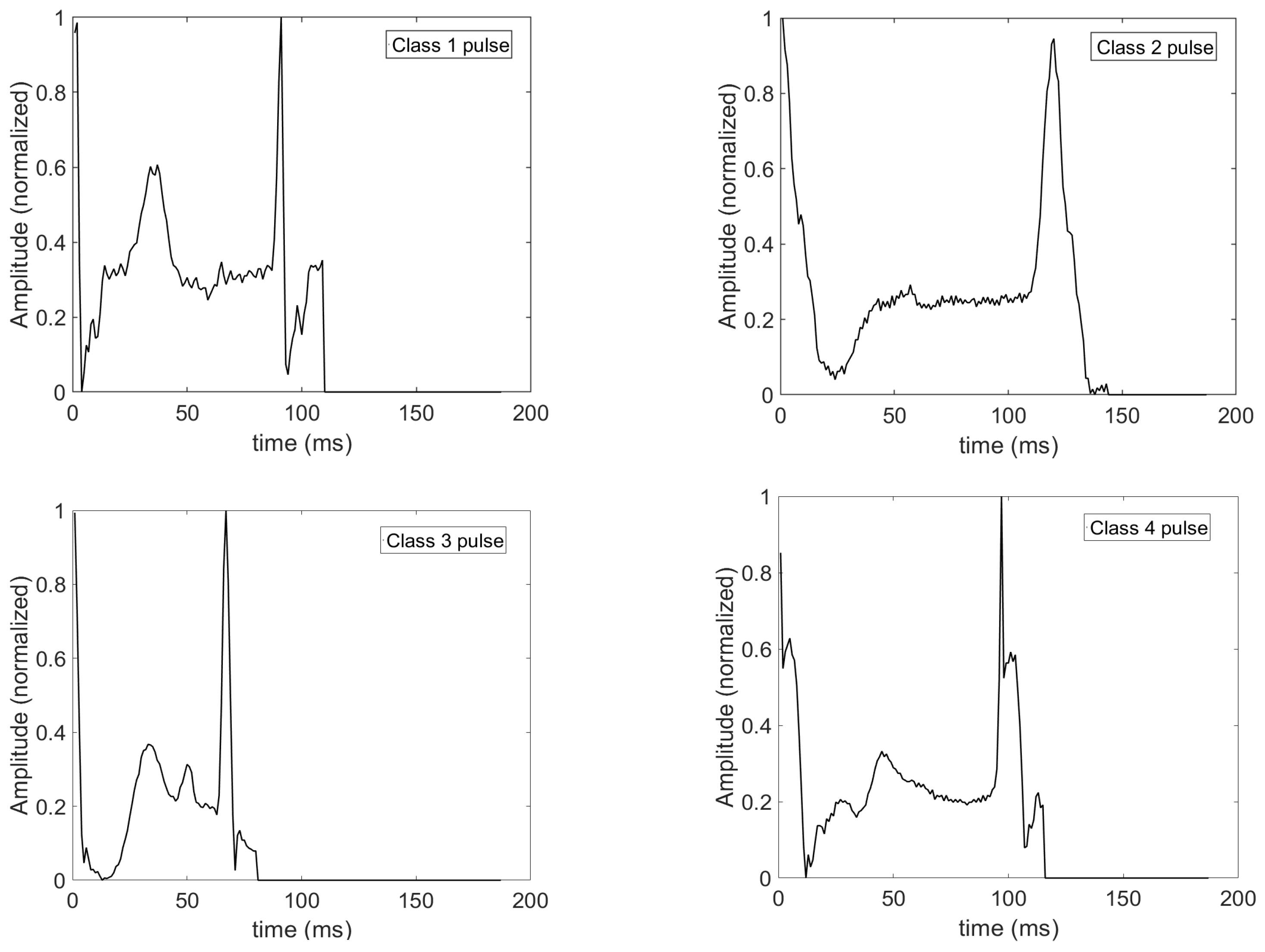
Figure 2. Example ECG segments from MIT–BIH arrhythmia database [18], one for each type of heartbeat class. (Top left): A schematic representation of an ECG pulse sequence. (Top right): Example of a class 0 pulse. (Middle row): Examples of class 1 and 2 pulses. (Bottom row): Examples of class 3 and 4 pulses.
Computation 14 00049 g002aComputation 14 00049 g002b
Figure 3. Bar chart of % accuracy values of optimized ESNs for successive steps of ESN optimization process. DF refers to a default ESN with unoptimized hyperparameter values α = 0.9, ρ = 1, and θ = 1.
Computation 14 00049 g003
Figure 4. Reservoir performance vs. total number of reservoir nodes. (Top): Average % accuracy across all classes and std. deviation of the % accuracies per class. (Bottom) % accuracy of the most and least successfully recognized classes.
Computation 14 00049 g004
Figure 5. Average % accuracy across all classes and std. deviation of the % accuracies per class vs. noise amplitude A (%).
Computation 14 00049 g005
Figure 6. Reservoir performance vs. variability of node transfer function. (Top): Overall accuracy and std. deviation vs. sigma bias. (Bottom): Overall accuracy and std. deviation vs. sigma gain.
Computation 14 00049 g006
Table 1. Optimal final values of basic ESN hyperparameters for the 300-node reservoir.
HyperparameterValue
Reservoir geometry Ring
Leaking rate (α) 1
Spectral radius (ρ) 0.2
Input weight scaling (θ) 4
Gain (G) 1
Bias (b) 1.5
Table 2. Comparison of heartbeat classification results with other studies. “N/A” stands for “Not Available” data. The boldfaced text is for emphasis.
WorkApproachOverall Accuracy (%)Max. Accuracy
per Class (%)
Min. Accuracy
per Class (%)
Measured Training Time on GPU 1Measured Training Time on CPU 2
This study1200 node ESN91.797.586.0N/A2.5 min
This study1800 node ESN93.498.187.6N/A6 min
This study3000 node ESN95.098.588.9N/A16 min
This study4800 node ESN96.399.190.2N/A40 min
[18]Deep residual CNN93.498.086.0120 min 12–3 days 3
[25]Augmentation + CNN93.5N/AN/AN/AN/A
[26]DWT + SVM93.8N/AN/AN/AN/A
[27]DWT + random forest94.6N/AN/AN/AN/A
1 On a GeForce GTX 1080Ti processor with TensorFlow Python computational library. 2 On an Intel i5-1235U@1.3GHz/DDR4 Windows 10 HP laptop using MATLAB script. It is estimated that it runs 25–30 times slower than a GeForce GTX 1080Ti GPU. 3 This is a rough estimate for the expected runtime, had the training procedure of reference [18] been run on our CPU machine (Intel i5-1235U@1.3GHz/DDR4 Windows 10 HP laptop) instead of their GeForce GTX 1080Ti processor and with our MATLAB v2024b scripts, mentioned in the text, instead of TensorFlow Python package. The reported times are based on a comparison between the relative capacities of the two hardware configurations.
Table 3. Reservoir geometry and its impact on Multi-ESN performance for N = 1200 nodes.
Reservoir GeometryAverage Accuracy (%)Std. Deviation of Class Accuracies (%)Max. Accuracy
per Class (%)
Min. Accuracy
per Class (%)
Ring91.824.4697.3286.26
Random (20% non-zero weights)91.324.7197.3385.85
Deep architecture—3 layers of random connectivity71.9317.1590.5047.59
Disclaimer/Publisher’s Note: The statements, opinions and data contained in all publications are solely those of the individual author(s) and contributor(s) and not of MDPI and/or the editor(s). MDPI and/or the editor(s) disclaim responsibility for any injury to people or property resulting from any ideas, methods, instructions or products referred to in the content.