Information Inequalities for Five Random Variables

Abstract

The entropic region is formed by the collection of the Shannon entropies of all subvectors of finitely many jointly distributed discrete random variables. For four or more variables, the structure of the entropic region is mostly unknown. We utilize a variant of the Maximum Entropy Method to obtain five-variable non-Shannon entropy inequalities, which delimit the five-variable entropy region. This method adds copies of some of the random variables in generations. A significant reduction in computational complexity, achieved through theoretical considerations and by harnessing the inherent symmetries, allowed us to calculate all five-variable non-Shannon inequalities provided by the first nine generations. Based on the results, we define two infinite collections of such inequalities and prove them to be entropy inequalities. We investigate downward-closed subsets of non-negative lattice points that parameterize these collections, and based on this, we develop an algorithm to enumerate all extremal inequalities. The discovered set of entropy inequalities is conjectured to characterize the applied method completely.

1. Introduction

Many important mathematical problems can be reduced to the following question: does a collection of finite random variables exist such that the entropies of the variable subsets satisfy certain linear constraints? Examples include, but are not limited to, channel coding [1] and network coding in particular [2], estimating the efficiency of secret sharing schemes [3,4,5], questions about matroid representations [6], guessing games [7], extracting information from common strings in cryptography [8], additive combinatorics [9], and finding conditional independence inference rules [10].

The entropy function of finitely many discrete random variables $\langle {\xi }_i:i\in N\rangle$ indexed by the fixed finite set N maps the non-empty subsets $I\subseteq N$ to the Shannon entropy $\mathbf{H}\left({\xi }_I\right)$ of the variable set ${\xi }_I=\langle x_i:i\in I\rangle$, see [11]. The entropy region, denoted by ${\Gamma }_N^{\ast }$, is the range of the entropy function; it is a part of the $2^{\left|N\right|}-1$-dimensional Euclidean space where the coordinates are labeled by non-empty subsets of N. Entropies are non-negative real numbers, and thus the entropy region lies in the non-negative orthant of this Euclidean space. It is delimited by a collection of homogeneous linear inequalities corresponding to the non-negativity of basic Shannon information measures [11]. Points satisfying all these inequalities form the Shannon-bound; the Shannon-bound is denoted by ${\Gamma }_N$.

N. Pippenger argued in [12] that linear inequalities bounding the entropic region ${\Gamma }_N^{\ast }$ encode the fundamental laws of Information Theory and determine the limits of information transmission and data compression. The long-standing problem of whether a linear information inequality can properly cut into the Shannon bound was settled in 1998 by Zhang and Yeung [13] who exhibited the first example of such a non-Shannon information inequality. Their discovery initiated intensive research. The phrase Copy Lemma was coined by Dougherty et al. [14] to describe the general method distilled from the original Zhang–Yeung construction. The Copy Lemma has been applied successfully to generate several hundred sporadic and a couple of infinite families of non-Shannon entropy inequalities for ${\Gamma }_4^{\ast }$, see [14,15,16]. A different method, utilizing an information-theoretic lemma attributed to Ahlswede and Körner [17], was proposed in [18]; later it was shown to be equivalent to a special case of the Copy Lemma [19].

Our method to obtain five-variable non-Shannon entropy inequalities is based on a more general paradigm of which the Copy Lemma is a special case [20]. Derived from the principle of maximum entropy [21], it is called MEM, short for Maximum Entropy Method. For more details, see Section 3.

Previous works on generating and applying non-Shannon entropy inequalities, such as [4,10,14,15,22,23], focused on the four-variable case, and only a few sporadic five-variable non-Shannon inequalities have been discovered, such as the MMRV inequality from [18]. This is the first work that provides a method that generates an infinite collection of non-Shannon bounds on the five-variable entropy region ${\Gamma }_5^{\ast }$. Compared to the four-variable case, there are significant challenges, both theoretical and computational. The four-variable entropy region ${\Gamma }_4^{\ast }$ sits in the 15-dimensional Euclidean space, while the five-variable region ${\Gamma }_5^{\ast }$ is 31-dimensional. The structure of the Shannon bound ${\Gamma }_4$ is well-understood: it has 41 extremal directions, and only 6 of them have no entropic points. The entropy region ${\Gamma }_4^{\ast }$ has an inner polyhedral cone where it fills its Shannon bound, and has six isomorphic “protrusions” towards the six exceptional extremal directions, each protrusion surrounded by 15 hyperplanes of which 14 come from the Shannon bound [24]. Only the protrusions contribute to new entropy inequalities, and their dimension can be reduced to 10. Computational results about ${\Gamma }_4^{\ast }$ can be obtained by computing vertices and facets of numerous implicitly defined 10-dimensional polyhedra [22]. In contrast, the Shannon bound ${\Gamma }_5$ of the five-variable entropy region has 117,983 extremal directions [25], and for a few of them it is not even known whether they contain an entropic point or not. No structural reduction similar to the four-variable case is available, and it is not known whether such a reduction exists or not. Computations about ${\Gamma }_5^{\ast }$ can still be reduced to 25-dimensional polyhedral enumeration problems (although with significantly larger number of constraints than in the 4-variable case). The complexity of enumeration problems typically doubles when the dimension increases by one, making such high-dimensional enumeration problems practically intractable.

We overcome this computational difficulty by applying a particular variant of the Maximum Entropy Method. This variant, working in generations, first reduces the problem dimension from 31 to 19, and then, at each generation, adds extra copies of some of the random variables, increasing the problem dimension again. Theoretical considerations and harnessing the inherent symmetry allowed us to complete the associated polyhedral computations up to nine generations. The output was the complete list of five-variable non-Shannon inequalities provided by the first nine generations. Based on the experimental results, we define an infinite collection of five-variable inequalities that we prove are provided by this MEM variant—in particular, they are valid non-Shannon entropy inequalities—and conjecture this collection to be complete; that is, no additional inequalities are yielded by this MEM variant. The collection of the inequalities is parametrized by finite, downward closed subsets of the non-negative lattice points of the plane. Some of the inequalities in our collection are consequences of the others; those that are not, are called extremal. We developed an incremental algorithm that enumerates, from generation to generation, the parameters yielding the extremal inequalities, in complete agreement with the computational results. The algorithm allowed us to significantly exceed the capabilities of polyhedral computation. While numerical instability prevented the completion of the polyhedral computation for the tenth generation, all extremal entropy inequalities were enumerated up to generation 60. Finally, we have examined the large-scale behavior of the extremal inequalities, and depicted how these inequalities delimit a three-dimensional cross-section of ${\Gamma }_5^{\ast }$.

The new five-variable non-Shannon inequalities can be applied to real-world problems. The most immediate application is in network coding. The new inequalities tighten the boundaries; they provide stricter and more accurate bounds on network capacity. In a network protocol they can assist in proving whether a targeted data rate is achievable or not [2].

Cloud storage services (like Google Drive or AWS S3) distribute data fragments across many nodes [26]. In case of failure, the node has to download the missing data from other nodes. The new five-variable inequalities can be used to determine the theoretical limits of storage efficiency for systems with more complex failure models or larger clusters.

In the realm of secret sharing, entropy inequalities provide lower bounds on the size of secrets [3,4,5]. To explore another facet of these problems, the new inequalities can prove that certain efficient schemes are impossible to realize. In complex datasets, it is important to distinguish between correlation and actual causation [27]. When an AI model analyzes data to build a causal graph, it can use entropy inequalities to rule out models that are information-theoretically impossible, narrowing the search space and improving accuracy.

In this paper lemmas, claims and theorems are arranged so that each is used in the same section only, typically right after they are stated and proved. Section 4 proves structural properties of the entropy region that are used to reduce the computational complexity of the polyhedral algorithms. The main theoretical results are stated and proved in Section 7. In Theorem 1 we prove a large collection of entropy inequalities parametrized by the downward-closed subsets of the non-negative lattice points. Lemmas estimating different entropy expressions are used in this section only. Unfortunately, many inequalities provided by Theorem 1 are consequences of the others. Claims and lemmas in Section 8 provide the theoretical foundation for our algorithm that selects and enumerates the extremal inequalities among them.

The remaining part of the paper is organized as follows. Notations are recalled in Section 2. Section 3 describes the special variant of the Maximum Entropy Method we apply to ${\Gamma }_5^{\ast }$. Section 4 discusses possible simplifications, including how symmetry can be utilized and how the MEM parameters were chosen. Section 5 describes the chosen coordinate systems, polyhedral computations, and their results. Section 6 presents the five-variable inequalities we obtained, paving the way for the definition of two infinite families of such inequalities in Section 7. Additional theoretical results, including the proof that inequalities in these families are indeed generated by the MEM method, are presented in Section 7. Section 8 discusses methods that can recognize extremal inequalities, discusses the incremental algorithm that enumerates the extremal inequalities for each MEM generation, describes the large-scale behavior of the new inequalities, and investigates the delimited part of the five-variable entropy region. Finally, Section 9 summarizes our work, lists open questions, and provides directions for further work.

2. Preliminaries

In this paper all sets are finite. Capital letters, such as A, J, N, etc., denote (finite) sets; elements of these sets are denoted by lower case letters. The union sign and the curly brackets around singletons are frequently omitted, thus, $Nij$ denotes the set $N\cup \{i,j\}$. The difference of two sets is written as $A-B$, or $A-b$ if the second set is a singleton. The star in the union $A{\cup }^{\ast }B$ emphasizes that A and B are disjoint sets. A partition of N is a collection of non-empty disjoint subsets of N whose union equals N.

A discrete random variable ξ takes its values from a finite set $\mathcal{X}$, called alphabet. The probability that $\xi$ takes $x\in \mathcal{X}$ is denoted by $\mathrm{Pr}(\xi =x)$, or simply by $\mathrm{Pr}\left(x\right)$ when the random variable $\xi$ is clear from the context. Suppose $\xi$ is defined on the direct product $\mathcal{X}={\prod }_{i\in N}{\mathcal{X}}_i$ for some finite set N, called the base set. For a non-empty $A\subseteq N$ the marginal ${\xi }_A$ is defined on the product alphabet ${\mathcal{X}}_A={\prod }_{i\in A}{\mathcal{X}}_i$ so that the probability of $y\in {\mathcal{X}}_A$ is the sum of the probabilities of those $x\in \mathcal{X}$ whose projection to ${\mathcal{X}}_A$ equals y:

$$\mathrm{Pr}(y)=\sum \{\mathrm{Pr}(x):x\upharpoonright A=y\}.$$

(1)

To emphasize that $\xi$ is defined on a product space, we write $\xi =({\xi }_i:i\in N)$, and say that the random variables ${\xi }_i$ are distributed jointly. The Shannon entropy of the distribution $\xi$ is defined as

$$\mathbf{H}\left(\xi \right)=\sum _{x\in \mathcal{X}}-\mathrm{Pr}\left(x\right)\log \mathrm{Pr}\left(x\right)$$

(2)

with the convention that $0\log 0=0$. If $\xi =({\xi }_i:i\in N)$ is a joint distribution, then we write ${\mathbf{H}}_{\xi }\left(A\right)$ for $\mathbf{H}\left({\xi }_A\right)$. The index $\xi$ is also dropped when it is clear from the context. By convention, $\mathbf{H}(\varnothing )=0$. The entropies ${\mathbf{H}}_{\xi }\left(A\right)$ are arranged into a vector indexed by the non-empty subsets A of N. This vector is the entropy profile of the distribution $\xi$. The collection of these $(2^{\left|N\right|}-1)$-dimensional vectors forms the entropy region, denoted by ${\Gamma }_N^{\ast }$. Elements of ${\Gamma }_N^{\ast }$ are considered interchangeably as vectors, as points in this Euclidean space, and as functions assigning non-negative real numbers to non-empty subsets of the base set N. For a gentle introduction to these notions of Information Theory, please consult [11].

Notions of conditional entropy, mutual information, and conditional mutual information from Information Theory are formally extended to the functional form of these vectors. If f is any function on subsets of N, then for subsets $A,B,C,D$ of N the following forms will be used as abbreviations:

$$\begin{array}{cc}\hfill f\left(A\right|B)& \stackrel{\mathrm{def}}{=}f\left(AB\right)-f\left(B\right),\hfill \\ \hfill f(A,B)& \stackrel{\mathrm{def}}{=}f\left(A\right)+f\left(B\right)-f\left(AB\right),\hfill \\ \hfill f(A,B|C)& \stackrel{\mathrm{def}}{=}f\left(AC\right)+f\left(BC\right)-f\left(ABC\right)-f\left(C\right), \mathrm{and}\hfill \\ \hfill f[A,B,C,D]& \stackrel{\mathrm{def}}{=}-f(A,B)+f(A,B|C)+f(A,B|D)+f(C,D).\hfill \end{array}$$

The first three expressions are called conditional entropy, mutual information, and conditional mutual information, respectively. The last line defines the Ingleton expression. An entropy function is not defined on the empty set, nevertheless, $f(\varnothing )=0$ will be assumed whenever convenient. In particular, $f(A,B|\varnothing )$ and $f(A,B)$ are the same expressions. Frequently, when clear from the context, the function f is omitted before the parenthesized expression. Additionally, if applied to singletons, the Ingleton expression is written without commas. An example is the inequality

$$\left[abcd\right]+(a,b|z)+(b,z\left|a\right)+(a,z|b)+3(z\left|ab\right)⩾0.$$

(3)

Shannon inequalities state the non-negativity of the conditional entropy, mutual information, and conditional mutual information for all subsets A, B, C of the base set N. They are consequences of the unique minimal set of such inequalities, called basic Shannon inequalities, see [11], listed in (B1) and (B2) below:

(B1)

$f\left(i\right|N-i)⩾0$ for all $i\in N$;

(B2)

$f(a,b|K)⩾0$ for all $K\subseteq N$ and different $a,b\in N-K$, including $K=\varnothing$.

The collection of all $(2^{\left|N\right|}-1)$-dimensional vectors (or points, or functions) that satisfy the Shannon inequalities is denoted by ${\Gamma }_N$. It is a natural outer bound for the entropy region ${\Gamma }_N^{\ast }$. ${\Gamma }_N$ is a pointed polyhedral cone [28]; its facets are the hyperplanes specified by the basic Shannon inequalities. Polymatroids are elements of ${\Gamma }_N$ written in functional form. A polymatroid is usually written as $(f,N)$, or just f, when we say that f is on N. The polymatroid f is entropic if it is in ${\Gamma }_N^{\ast }$, and almost entropic, or aent for short, if it is in the closure (in the usual Euclidean topology) of ${\Gamma }_N^{\ast }$. Linear inequalities valid for all polymatroids are consequences of the basic Shannon inequalities; an example is the inequality (3). A non-Shannon inequality is a homogeneous linear inequality that is valid for points of the entropic region but not for all points of the Shannon bound. Equivalently, the non-negative side of the hyperplane corresponding to such an inequality contains the complete entropy region, while it cuts properly into ${\Gamma }_N$.

The closure of the entropic region is a pointed convex full-dimensional cone [11], and only its boundary points can be non-entropic [29].

The polymatroid $(f,N)$ on the base set N is linearly representable over the field $\mathbb{F}$, or  $\mathbb{F}$-representable in short, if there is a finite-dimensional vector space V over $\mathbb{F}$, and linear subspaces $V_i\subseteq V$ for $i\in N$, such that for all $I\subseteq N$, $f\left(I\right)$ is the dimension of the linear subspace spanned by ${\bigcup }_{i\in I}{V}_i$. Clearly, if both $(f,N)$ and $(g,N)$ are $\mathbb{F}$-representable over the same field, then so is their sum $f+g$. The polymatroid f is $\mathbb{F}$-linear if it is in the closure of the multiplies of $\mathbb{F}$-representable polymatroids. By the previous remark, $\mathbb{F}$-linear polymatroids form a closed cone. Finally, f is linear if it is $\mathbb{F}$-linear for some field $\mathbb{F}$.

Following a compactness argument, if f is $\mathbb{F}$-representable, then it is representable over some finite field as well, see [30], meaning that the vector space V is also finite. Taking the uniform distribution on V provides the entropic polymatroid $\left(\log \right|V\left|\right)f$. Thus, linear polymatroids are also almost entropic.

Linear polymatroids on the base set N with $\left|N\right|⩽5$ are $\mathbb{F}$-linear for every field $\mathbb{F}$, see [24,31]; this statement is not true in general. For $\left|N\right|⩽3$ every polymatroid is linear. For $N=\left\{abcd\right\}$ a polymatroid f on N is linear if and only if it satisfies the following six instances of the Ingleton inequality:

$$\begin{array}{ccc}f\left[abcd\right]⩾0,& f\left[acbd\right]⩾0,& f\left[adbc\right]⩾0,\\ f\left[bcad\right]⩾0,& f\left[bdac\right]⩾0,& f\left[cdab\right]⩾0,\end{array}$$

(4)

see [24]. Since the Ingleton expression is symmetric in the first two and in the last two arguments, these expressions cover all 24 permutations of N.

Finally, we recall notions of independence. Let $(f,N)$ be a polymatroid, and X, $Y_1$, …, $Y_k$ be disjoint subsets of N. $Y_1$ and $Y_2$ are independent in f if $f(Y_1,Y_2)=0$. The collection $Y_1,\dots ,Y_k$ is completely independent in f if for any two disjoint subsets I and J of the indices $\{1,2,\dots ,k\}$, $Y_I={\bigcup }_{i\in I}{Y}_i$ and $Y_J$ are independent, or, equivalently, if 

$$f(Y_1\cdots Y_k)=f\left(Y_1\right)+\cdots +f\left(Y_k\right).$$

(5)

In this case we also have $f\left(Y_I\right)={\sum }_{i\in I}f\left(Y_i\right)$ for every subset I of the indices. The disjoint subsets $Y_1$ and $Y_2$ are conditionally independent over X if $f(Y_1,Y_2|X)=0$; and $Y_1,\dots ,Y_k$ are completely conditionally independent over X if $Y_I$ and $Y_J$ are conditionally independent over X for arbitrary disjoint subsets I and J of the indices. An equivalent condition is

$$f(Y_1\cdots Y_k|X)=f\left(Y_1\right|X)+\cdots +f\left(Y_k\right|X),$$

(6)

which similarly implies $f\left(Y_I\right|X)={\sum }_{i\in I}f\left(Y_i\right|X)$ for every index set I.

3. The Maximum Entropy Method

In general terms, the principle of maximum entropy is easy to formulate: if a probability distribution is specified only partially, take the one with the largest entropy, see, e.g., [21]. In the particular case applied here “partial specification” means fixing some, but not all, marginal distributions. To be more concrete, suppose $\xi$ is distributed jointly on the base set N. Partition N into three non-empty subsets as $N=Y{\cup }^{\ast }X{\cup }^{\ast }Z$. Take $n⩾1$ disjoint copies of Y and $m⩾1$ disjoint copies of Z to form the enlarged base set

$$N^{\ast }=Y_1{\cup }^{\ast }\cdots {\cup }^{\ast }{Y}_n{\cup }^{\ast }X{\cup }^{\ast }{Z}_1{\cup }^{\ast }\cdots {\cup }^{\ast }{Z}_m.$$

(7)

Consider the collection of those distributions ${\xi }^{\ast }$ on $N^{\ast }$ whose marginals on $Y_{i}X$ are equal to ${\xi }_{YX}$, and marginals on $X{Z}_j$ are equal to ${\xi }_{XZ}$. That is, the marginal of $\xi$ on $YX$ and the marginals of ${\xi }^{\ast }$ on all $Y_{i}X$ are the same as well as the marginal of $\xi$ on $XZ$ and the marginals of ${\xi }^{\ast }$ on $X{Z}_j$. This collection of distributions is not empty, as one can take each $Y_i$ to be the same as Y, and each $Z_j$ to be the same as Z. The total entropy is a strictly concave function of the probability masses, and fixing certain marginals imposes linear constraints on those masses. Consequently, there is a unique optimal distribution ${\xi }^{\ast }$ with maximum total entropy, see [32]. Although structural properties of the maximum entropy distributions are mainly unknown, they are known to satisfy numerous conditional independencies. For this particular case, these are stated as Lemma 1 below.

Lemma 1.

In the distribution with maximum total entropy, the subsets $Y_1,\dots ,Y_n$ and $Z_1,\dots ,Z_m$ are completely conditionally independent over X.

Proof. 

If some of the conditional independence statements do not hold, then one can redefine the distribution keeping the specified marginals while increasing the total entropy. For details, see [20]. □

Since identical distributions have identical entropy profiles, Lemma 1 immediately implies that an entropic polymatroid has an $n,m$-copy as defined below:

Definition 1.

Let f be a polymatroid on N, and partition N into three non-empty subsets as $N=Y{\cup }^{\ast }X{\cup }^{\ast }Z$. Let $Y_1,\dots ,Y_n$ and $Z_1,\dots ,Z_m$ be disjoint copies of Y and Z, respectively. The polymatroid $f^{\ast }$ on the base set $N^{\ast }=Y_1\dots Y_{n}X{Z}_1\dots Z_m$ is an $n,m$-copy of f if

(i) 

$f^{\ast }$ restricted to $Y_{i}X$ is isomorphic to $f\upharpoonright YX$ for every $i⩽n$,

(ii) 

$f^{\ast }$ restricted to $X{Z}_j$ is isomorphic to $f\upharpoonright XZ$ for every $j⩽m$,

(iii) 

the $n+m$ subsets $Y_1,\dots ,Y_n,Z_1,\dots ,Z_m$ are completely conditionally independent over X in $f^{\ast }$.

The special version of the Maximum Entropy Method used in this paper is based on the fact that entropic polymatroids have $n,m$-copies. For fixed integers n and m, polymatroids on $YXZ$ that have an $n,m$-copy form a polyhedral cone ${\mathcal{C}}_{n,m}$. This is proved as Claim 1 below. The cone ${\mathcal{C}}_{n,m}$ contains the complete entropy region ${\Gamma }_{YXZ}^{\ast }$, and is contained in the Shannon cone ${\Gamma }_{YXZ}$. Consequently, bounding facets of the cone ${\mathcal{C}}_{n,m}$ that are not facets of the Shannon cone provide new entropy inequalities. This method is summarized as follows.

Maximum Entropy Method

(special case). Fix the base set N and the partition $N=Y{\cup }^{\ast }X{\cup }^{\ast }Z$. For $n,m⩾1$ let ${\mathcal{C}}_{n,m}$ be the polyhedral cone of those polymatroids on N that have an $n,m$-copy. Compute all bounding facets of ${\mathcal{C}}_{n,m}$ as homogeneous linear inequalities, and delete those which are consequences of the basic Shannon inequalities. The remaining inequalities form the maximal set of non-Shannon inequalities provided by the partition $YXZ$ and the numbers n and m.

Let us remark that while the maximum entropy extension is unique, the $m,n$-copy in Definition 1 is typically not, as the definition captures only a small part of the properties of the maximum entropy extension. The obtained entropy inequalities form the facets of a convex polytope; consequently, they are independent in the sense that none of them is a consequence of the others or the Shannon inequalities.

Next we prove that ${\mathcal{C}}_{n,m}$ is a polyhedral cone indeed.

Claim 1.

Polymatroids $(f,N)$ with an $n,m$-copy form a polyhedral cone.

Proof. 

Consider the polymatroid f as a $(2^{\left|N\right|}-1)$-dimensional vector indexed by the non-empty subsets of N. Write this vector as $(\mathbf{x},\mathbf{u})$ where $\mathbf{x}$ of dimension $d_1$ contains those coordinates where the index I is a subset of either $YX$ or $XZ$, and $\mathbf{u}$ of dimension $d_2$ contains the rest, namely those subsets that intersect both Y and Z. Clearly, $d_1+d_2=2^{\left|N\right|}-1$. Similarly, let $\mathbf{y}$ be the vector formed from the values of the $n,m$-copy polymatroid $f^{\ast }$ as indexed by the subsets of $N^{\ast }$. The vector $\mathbf{y}$ has dimension $d_3=2^{|N^{\ast }|}-1$. Now, $(f^{\ast },N^{\ast })$ is a polymatroid if the vector $\mathbf{y}$ satisfies all linear inequality constraints imposed by the basic Shannon inequalities in (B1) and (B2); and it is an $n,m$-copy of f if, additionally, the composed vector $(\mathbf{x},\mathbf{y})$ satisfies the equality constraints corresponding to conditions (i)–(iii) in Definition 1. Consequently, there exists a matrix M with $d_1+d_3$ columns, depending only on the partition $YXZ$ and the numbers n and m, so that f has an $n,m$-copy if and only if there is a vector $\mathbf{y}$ satisfying $M·{(\mathbf{x},\mathbf{y})}^{\top }⩾0$. Similarly, $(f,N)$ is a polymatroid if, for another matrix B with $(d_1+d_2)$ columns expressing the basic Shannon inequalities for $YXZ$, we have $B·{(\mathbf{x},\mathbf{u})}^{\top }⩾0$. Thus the collection of polymatroids on N that have an $n,m$-copy is the set

$$\begin{array}{cc}\hfill \mathcal{Q}=\{(\mathbf{x},\mathbf{u})\in {\mathbb{R}}^{d_1+d_2}:& B·{(\mathbf{x},\mathbf{u})}^T⩾0, \mathrm{and}\hfill \\ \hfill & M·{(\mathbf{x},\mathbf{y})}^{\top }⩾0 \mathrm{for} \mathrm{some} \mathbf{y}\in {\mathbb{R}}^{d_3}\}.\hfill \end{array}$$

Here M and B are matrices with integer entries; these matrices depend only on $YXZ$, n, and m. Since $\mathcal{Q}$ is the intersection of a polyhedral cone and the projection of a polyhedral cone, it is also a polyhedral cone, as claimed. □

From the proof it is clear that the $\mathbf{u}$-part of $\mathcal{Q}$ is constrained only by the basic Shannon inequalities encoded in the matrix B. Furthermore, constraints on $\mathbf{x}$ imposed by the first condition are contained in the second one. Thus, it suffices to consider the bounding facets of

$${\mathcal{Q}}^{\ast }=\left\{\mathbf{x}\in {\mathbb{R}}^{d_1}:M·{(\mathbf{x},\mathbf{y})}^{\top }⩾0 \mathrm{for} \mathrm{some} \mathbf{y}\in {\mathbb{R}}^{d_3}\right\}$$

(8)

for new entropy inequalities. This is because, due to the duality theorem of linear programming [28], facets of $\mathcal{Q}$ are convex linear combinations of facets of ${\mathcal{Q}}^{\ast }$ and facets corresponding to the basic Shannon inequalities for the base set $YXZ$.

Coordinates in $\mathbf{x}$ are indexed by subsets of $YX$ and $XZ$, so the inequalities provided by the bounding facets of ${\mathcal{Q}}^{\ast }$ contain only elements of the restrictions $f\upharpoonright YX$ and $f\upharpoonright XZ$. We emphasize that these restrictions are not arbitrary polymatroids on $YX$ and $XZ$ with a common restriction on X, as they also have a common extension, namely f. Conditions ensuring the existence of such a common extension are assumed to hold, see [33], and they do not contribute towards the non-Shannon entropy inequalities we are searching for.

4. What to Compute? How to Compute?

As discussed in Section 3, the task of finding new non-Shannon entropy inequalities implied by the existence of an $n,m$-copy reduces to enumerating all facets of the polyhedral cone ${\mathcal{Q}}^{\ast }$ defined in (8). However, without further reduction, this polyhedral computation is intractable even for small parameter values. Therefore, in this section we look at some general methods to reduce the complexity of the computation, and then discuss how the number of elements in the $YXZ$ partition was chosen.

4.1. Tight and Modular Parts

Both the polyhedral region ${\Gamma }_N$ and the closure of the entropy region $\overline{{\Gamma }_N^{\ast }}$ decompose naturally into direct sums of modular and tight parts, see [23]. To discuss this result, let us first introduce some notation. For $i\in N$ define the function ${\mathit{r}}_i$ on the non-empty subsets A of N as

$${\mathit{r}}_i:A\mapsto \left\{\begin{array}{cc}1\hfill & \mathrm{if} i\in A,\hfill \\ 0\hfill & \mathrm{otherwise}.\hfill \end{array}\right.$$

(9)

Non-negative multiples of ${\mathit{r}}_i$ are clearly entropic polymatroids; modular polymatroids are, by definition, the conic combinations of the vectors $\{{\mathit{r}}_i:i\in N\}$. For a polymatroid $(f,N)$, a singleton $i\in N$ and a real number $\alpha ⩾0$, the function $f{\downarrow }_{\alpha }^i$ is defined on the non-empty subsets of N as follows:

$$f{\downarrow }_{\alpha }^i:A\mapsto \min \{f\left(Ai\right)-\alpha ,f\left(A\right)\}.$$

(10)

When $\alpha$ is set to $f\left(i\right|N-i)$, $f{\downarrow }_{\alpha }^i$ is denoted simply by $f{\downarrow }^i$. Note that for $i\notin A$ we have $f\left(Ai\right)-f\left(A\right)⩾f\left(N\right)-f(N-i)=f\left(i\right|N-i)$ by submodularity. Consequently, $f{\downarrow }^i$ can be written explicitly as

$$f{\downarrow }^i\left(A\right)=\left\{\begin{array}{cc}f\left(A\right)-f\left(i\right|N-i)\hfill & \mathrm{if} i\in A,\hfill \\ f\left(A\right)\hfill & \mathrm{if} i\notin A.\hfill \end{array}\right.$$

(11)

Therefore, $f=f{\downarrow }^i+ f\left(i\right|N-i){\mathit{r}}_i$, where ${\mathit{r}}_i$ is the polymatroid defined in (9). The result of tightening f at i is the function $f{\downarrow }^i$. The tight part of f, denoted by $f\downarrow$, is the result of tightening f at every element of its base set $N=\{i_1,\dots ,i_n\}$:

$$f\downarrow =(\cdots (f{\downarrow }^{i_1}){\downarrow }^{i_2}\cdots ){\downarrow }^{i_n}.$$

(12)

This result is independent of the order in which the reductions are applied, which is also shown by the decomposition formula

$$f=f\downarrow +\sum _{i\in N}f\left(i\right|N-i){\mathit{r}}_i.$$

(13)

The proof of the following lemma can be found in [20] or [34]. In this paper only the first part of the lemma is needed, which can be verified by direct computation.

Lemma 2.

Let $0⩽\alpha ⩽f\left(i\right)$. If f is a polymatroid, then $f{\downarrow }_{\alpha }^i$ is also a polymatroid. If, in addition, f is almost entropic, then so is $f{\downarrow }_{\alpha }^i$. □

Accordingly, $f\downarrow$ (the tight part of f) is a polymatroid, and it is also almost entropic (aent) whenever f is aent. The difference $f-f\downarrow$ is the modular part, and it is a modular polymatroid. This decomposition of f into a tight and a modular part is unique, and both parts are aent if f is aent.

The cone formed by the modular polymatroids over N is $\left|N\right|$-dimensional, and is generated by the linearly independent vectors $\{{\mathit{r}}_i:i\in N\}$. The cone of tight polymatroids is orthogonal to this (modular) cone, and so to every vector ${\mathit{r}}_i$, and is bounded by the hyperplanes corresponding to the basic Shannon inequalities in (B2). The cone of tight, almost entropic polymatroids is similarly orthogonal to the modular cone. A consequence of this decomposition is that linear bounds on the entropic cone also decompose into bounds on the tight part and bounds on the modular part—the latter being trivial, that is, a Shannon inequality. The normal $\mathbf{n}$ of a supporting hyperplane of the tight part is necessarily orthogonal to all vectors ${\mathit{r}}_i$, that is, the scalar products $\mathbf{n}·{\mathit{r}}_i$ are zero. Consequently, if the normal has the coordinates $\mathbf{n}=\langle t_I:I\subseteq N\rangle$, then the sum $\sum \{t_I:i\in I\}$ is zero for every $i\in N$. For this reason, these hyperplanes are called balanced. The tight component of any entropy inequality is balanced, and it is also an entropy inequality. This fact is equivalent to saying that every entropy inequality can be strengthened to become a balanced one, see [35].

From the above it follows that the facets of the cone ${\mathcal{Q}}^{\ast }$ belong to two disjoint groups. There are $\left|N\right|$ (trivial, Shannon) facets that bound the modular part of ${\mathcal{Q}}^{\ast }$, and the rest bound the tight part. The normal vectors of the facets in the second group are balanced, and only they can provide non-Shannon inequalities. Therefore, it suffices to consider only the tight part of ${\mathcal{Q}}^{\ast }$. This part is generated by a smaller collection of polymatroids, has fewer dimensions, and so can be handled more efficiently.

Claim 2.

The tight part of ${\mathcal{Q}}^{\ast }$ is generated by the $n,m$-copies of the polymatroids f on $N=YXZ$ that are (i) tight; (ii) satisfy $f(Y,Z|X)=0$; and (iii) for all $y\in Y$, $f\left(y\right|YX-y)=0$, and for all $z\in Z$, $f\left(z\right|XZ-z)=0$.

Observe that the tightness of f at the elements of Y and Z follows from condition (iii) and submodularity; thus, (i) is relevant only for elements of X.

Proof. 

Let $f^{\ast }$ be an $n,m$-copy of f. In the definition of ${\mathcal{Q}}^{\ast }$ only the values of $f\upharpoonright YX$ and the values of $f\upharpoonright XZ$ are used. Therefore, f can be replaced with any other polymatroid that has the same restrictions. Such a polymatroid is $f^{\ast }\upharpoonright Y_{1}X{Z}_1$ by part (i) of Definition 1, which gives (ii). For (iii) let $y\in Y$, and $\alpha =f\left(y\right|YX-y)$. Apply Lemma 2 to $f^{\ast }$ and all instances of y in the copies $Y_i$ to get the new polymatroid $g^{\ast }$. Denoting the instance of y in $Y_1$ by $y_1$, the lemma provides $g^{\ast }\left(y_1\right|Y_{1}X-y_1)=0$. In addition, $g^{\ast }$ is an $n,m$-copy of its restriction to $Y_{1}X{Z}_1$. Since this restriction and the polymatroid f differ only by a modular shift on subsets of $YX$ and $XZ$, their tight parts are the same. A similar reduction on elements of Z, and finally on elements of X, provides the statement. □

Using Claim 2, the number of columns in the constraint matrix M in (8) can be significantly reduced. It is so since, by the tightness of f, $f^{\ast }\left(Ai\right)=f^{\ast }\left(A\right)$ holds for many subsets A of $N^{\ast }$ with few elements, and this equality implies $f^{\ast }\left(Bi\right)=f^{\ast }\left(B\right)$ for every $A\subseteq B\subset N^{\ast }$.

4.2. Symmetry

The inherent symmetry in the $n,m$-copy allows for another significant complexity reduction. Let $\pi$ be one of the $(n!m!)$ permutations of the base set $N^{\ast }$ that permutes the subsets $Y_i$ and the subsets $Z_j$ independently. This permutation naturally extends to the subsets of $N^{\ast }$, and then to the polymatroids on $N^{\ast }$. The $n,m$-copy $f^{\ast }$ of f is symmetric if it is invariant for each such permutation $\pi$, that is, $f^{\ast }\left(A\right)=\left(\pi f^{\ast }\right)\left(A\right)=f^{\ast }\left(\pi A\right)$ for all $A\subseteq N^{\ast }$.

Claim 3.

f has an $n,m$-copy if and only if it has a symmetric $n,m$-copy.

Proof. 

If $f^{\ast }$ is an $n,m$-copy of f, then clearly so is $\pi f^{\ast }$. Since conditions (ii) and (iii) in Definition 1 are linear, they are also satisfied by the average of all such permutations of $f^{\ast }$, that is, by the polymatroid $g^{\ast }={(n!m!)}^{-1}{\sum }_{\pi }\pi f^{\ast }$. Clearly, $g^{\ast }$ is a symmetric $n,m$-copy of f. □

Symmetry alone reduces the number of auxiliary variables in the definition of ${\mathcal{Q}}^{\ast }$ from exponential in n and m to polynomial in these parameters.

4.3. No New Inequality

In some cases, the computations required by the Maximum Entropy Method, as defined in Section 3, can be simplified further, or even completely avoided. The first claim of this subsection states that certain polymatroids do not contribute to new entropy inequalities.

Claim 4.

Suppose f is a polymatroid on $N=YXZ$, and f restricted to X is modular. Then f has an $n,m$-copy for every n and m.

Proof. 

The statement follows from the following lemma by induction. □

Lemma 3.

Suppose that the polymatroids $(f_1,YX)$ and $(f_2,XZ)$ have a common restriction on X which is modular. Then there is a polymatroid $(g,YXZ)$ that extends both $f_1$ and $f_2$ such that $g(Y,Z|X)=0$.

Proof. 

For $I\subseteq Y$, $J\subseteq X$ and $K\subseteq Z$ define

$$g\left(IJK\right)\stackrel{\mathrm{def}}{=}\underset{L}{\min }\{f_1\left(IL\right)+f_2\left(LK\right)-f_1\left(L\right):J\subseteq L\subseteq X\}.$$

(14)

Using the fact that $f_1\upharpoonright X$ and $f_2\upharpoonright X$ are isomorphic and modular, a simple calculation shows that g is a polymatroid and satisfies the requirements. For details, consult [20,33] or [29]. □

If either Y or Z has a single element, then one does not need to look beyond $n,1$-copies.

Claim 5.

Suppose $\left|Z\right|=1$. Entropy inequalities generated by $n,m$-copies of polymatroids on $YXZ$ are also generated by $n,1$-copies.

Proof. 

We claim that the cone generated by the tight part of $n,m$-copies is the same as the cone generated by the $n,1$-copies. To prove this, let f be a polymatroid on $YXZ$ that satisfies the conditions of Claim 2, and let $f^{\ast }$ be an $n,1$-copy of f so that f is identified with $f^{\ast }\upharpoonright Y_{1}X{Z}_1$ where $Z_1$ has a single element z. Let $g^{\ast }$ be the polymatroid when $m-1$ identical copies of z are added to $f^{\ast }$. We claim that $g^{\ast }$ is an $n,m$-copy. The only non-trivially satisfied condition is that the copies of z, $z_1$ and $z_2$, are independent over X. Since $f\left(z\right|X)=0$ by (iii) of Claim 2, we have $g^{\ast }\left(X{z}_1\right)=g^{\ast }\left(X{z}_2\right)=g^{\ast }\left(X{z}_1{z}_2\right)=g^{\ast }\left(X\right)$, thus $g^{\ast }(z_1,z_2|X)=0$. Since $g^{\ast }\upharpoonright Y_{1}X{Z}_1$ and $f^{\ast }\upharpoonright Y_{1}X{Z}_1$ are the same polymatroids, the $n,m$-cone is part of the $n,1$-cone, as claimed. □

4.4. Problem Parameters

By Claim 4, the Maximum Entropy Method does not yield new inequalities when $f\upharpoonright X$ is modular. This is certainly the case when $\left|X\right|=1$, so we must have $\left|X\right|⩾2$. By Claim 5, if $\left|Y\right|=\left|Z\right|=1$, then beyond the $1,1$-copy, no additional inequalities are generated. The smallest parameter setting when new entropy inequalities are expected as the number of copies grows is $\left|Y\right|=2$, $\left|X\right|=2$, and $\left|Z\right|=1$. We fix these sizes, as well as the labels of the members of each set as

$$X=\{a,b\},Y=\{c,d\},\mathrm{and} Z=\left\{z\right\}.$$

(15)

Since $\left|Z\right|=1$, according to Claim 5, it suffices to consider $n,1$-copies only. To simplify the notation, the extra 1 will be dropped and we write n-copy instead. We also explicitly state the definition of the n-copy for this particular partition.

Definition 2.

Let f be a polymatroid on $N=\left\{abcdz\right\}$, and let $n⩾1$. The polymatroid $f^{\ast }$ on the base set $N^{\ast }=abz\cup \{c_i{d}_i:1⩽i⩽n\}$ is an n-copy of f, if 

(i) 

$f^{\ast }\upharpoonright abz$ is isomorphic to $f\upharpoonright abz$, and, for each $i⩽n$, with the $c_i\leftrightarrow c$, $d_i\leftrightarrow d$ correspondences, $f^{\ast }\upharpoonright ab{c}_i{d}_i$ is isomorphic to $f\upharpoonright abcd$;

(ii) 

$\{c_i{d}_i:i⩽n\}$ and z are completely conditionally independent over $ab$.

This special case of the Maximum Entropy Method provides new non-Shannon entropy inequalities based on the fact that entropic polymatroids on the 5-element base set $abcdz$ have an n-copy for each $n⩾1$. The steps we will follow are as below:

• Fix the number of copies n, called a generation. Determine the generating matrix M of the cone ${\mathcal{Q}}^{\ast }$ as specified in Claim 1 using only polymatroids that satisfy the conditions of Claim 2.
• The new inequalities are provided by the non-Shannon facets of the tight part of ${\mathcal{Q}}^{\ast }$; these facets can be computed using some polyhedral algorithm from the generating matrix M.

5. Computation

The cone ${\mathcal{Q}}^{\ast }$ whose non-Shannon bounding facets provide the new entropy inequalities sits in the $d_1=19$-dimensional Euclidean space with coordinates indexed by the non-empty subsets of $YX=\left\{abcd\right\}$ and $XZ=\left\{abz\right\}$. Fix the number of copies to $n⩾1$. This choice also fixes the dimension $d_3$ of the vector $\mathbf{y}$. The generating matrix M of the polyhedral cone ${\mathcal{Q}}^{\ast }$ from (8) is repeated here:

$${\mathcal{Q}}^{\ast }=\left\{\mathbf{x}\in {\mathbb{R}}^{19}:M·{(\mathbf{x},\mathbf{y})}^{\top }⩾0 \mathrm{for} \mathrm{some} \mathbf{y}\in {\mathbb{R}}^{d_3}\right\}.$$

(16)

The modular part of ${\mathcal{Q}}^{\ast }$ is 5-dimensional, and so its tight part sits in a 14-dimensional subspace of ${\mathbb{R}}^{19}$.

A structural property of the polymatroid region on the four-element set $abcd$ allows us to further reduce the complexity of the polyhedral computation required in step (2) above. This region has a central part and six permutationally equivalent “protrusions,” depending on the signs of the Ingleton expressions

$$f\left[abcd\right],f\left[acbd\right],f\left[adbc\right],f\left[bcad\right],f\left[bdac\right], \mathrm{and} f\left[cdab\right].$$

(17)

If all of them are non-negative, then the restriction $f\upharpoonright abcd$ is a linear polymatroid; otherwise exactly one of these Ingleton expressions is negative, see e.g., [24]. Accordingly, the cone ${\mathcal{Q}}^{\ast }$ is cut into seven parts by these Ingleton hyperplanes: the central part where all Ingleton values are non-negative, and six other parts where exactly one of the expressions is negative. The facets of each part can be computed separately.

Parts of ${\mathcal{Q}}^{\ast }$ on the negative side of $\left[acbd\right]$, $\left[adbc\right]$, $\left[bcad\right]$, and $\left[bdac\right]$ are isomorphic because swapping $a\leftrightarrow b$ and/or $c\leftrightarrow d$ are symmetries of ${\mathcal{Q}}^{\ast }$. Therefore, it suffices to consider only one of them. The central part, where every Ingleton expression is non-negative, does not yield new inequalities. This follows from Lemma 4 below, as the elements of the central part are linear.

Lemma 4.

If f restricted to $abcd$ is linear, then f has an n-copy for all $n⩾1$.

Proof. 

Since every polymatroid on three elements is linear, and linearly representable polymatroids on three or four elements are representable over any field, we can assume, after scaling and using continuity, that both $f\upharpoonright abcd$ and $f\upharpoonright abz$ are $\mathbb{F}$-linearly representable over the same finite field $\mathbb{F}$. Denote the two representing vector spaces by $V^1$ and $V^2$, and consider the subspace arrangements $(V_a^1,V_b^1)$ and $(V_a^2,V_b^2)$ in the two vector spaces. Now $V_a^i$ and $V_b^i$ have dimensions $f\left(a\right)$ and $f\left(b\right)$, respectively, and their linear span has dimension $f\left(ab\right)$. Therefore, these arrangements are isomorphic, and $V^1$ and $V^2$ can be glued along the linear span of $(V_a^1,V_b^1)$ and $(V_a^2,V_b^2)$. This gluing yields an $\mathbb{F}$-linear polymatroid g that has the same restrictions on $abcd$ and on $abz$ as f does. Since this g is entropic, it has an n-copy for every $n⩾1$. This n-copy is also an n-copy of f, as required. □

Consequently, up to the $a\leftrightarrow b$ and $c\leftrightarrow d$ symmetries, three mutually exclusive cases are left: $f\left[abcd\right]<0$, $f\left[acbd\right]<0$, and $f\left[cdab\right]<0$. Using the homogeneity of ${\mathcal{Q}}^{\ast }$, the Ingleton value can be set to $-1$, in effect taking a cross-section of ${\mathcal{Q}}^{\ast }$ that has one fewer dimension. Facets of the part of ${\mathcal{Q}}^{\ast }$ we are considering are also facets of these cross-sections; consequently, only facets of the cross-sections need to be computed. We consider these three cases separately in the subsections below.

The definition (16) of the cone ${\mathcal{Q}}^{\ast }$ uses the 19-dimensional coordinate system where the coordinates of the vector $\mathbf{x}$ are labeled by the non-empty subsets of $abcd$ and $abz$. In all three cases we perform calculations in different coordinate systems that are chosen so that

• The first coordinate is the Ingleton expression defining the cross-section;
• The tight and modular parts of the cross-section have disjoint coordinates;
• Apart from the Ingleton coordinate, other coordinates have non-negative values.

The first property allows to set the Ingleton value explicitly. Based on the second property, the tight part of the cross-section can be separated by dropping some coordinates; and the third property potentially reduces the complexity of the polyhedral enumeration algorithm.

5.1. Case I

The cone ${\mathcal{Q}}^{\ast }$ is intersected with the hyperplane $\left[abcd\right]=-1$. In this case we use the coordinate system

$$\begin{array}{cc}{\mathsf{C}}_1:\hfill & \left[abcd\right],\hfill \\ {\mathsf{C}}_2-{\mathsf{C}}_4:\hfill & (a,b|c),\hfill & (a,c|b),\hfill & (b,c|a),\hfill \\ {\mathsf{C}}_5-{\mathsf{C}}_7:\hfill & (a,b|d),\hfill & (a,d|b),\hfill & (b,d|a),\hfill \\ {\mathsf{C}}_8-{\mathsf{C}}_{11}:\hfill & (c,d|a),\hfill & (c,d|b),\hfill & (c,d),\hfill & (a,b|cd),\hfill \\ {\mathsf{C}}_{12}-{\mathsf{C}}_{14}:\hfill & (a,b|z),\hfill & (a,z|b),\hfill & (b,z|a),\hfill \\ {\mathsf{C}}_{15}-{\mathsf{C}}_{19}:\hfill & \left(a\right|bcd),\hfill & \left(b\right|acd),\hfill & \left(c\right|abd),\hfill & \left(d\right|abc),\hfill & \left(z\right|ab).\hfill \end{array}$$

(18)

Coordinates ${\mathsf{C}}_{15}-{\mathsf{C}}_{19}$ cover the modular part of ${\mathcal{Q}}^{\ast }$. The tight part is spanned by the coordinate vectors ${\mathsf{C}}_1-{\mathsf{C}}_{14}$, and each of these vectors is orthogonal to the modular part. Let ${\tilde{P}}_1$ be the inverse of the matrix of this coordinate transformation, and the vector ${\mathbf{p}}_1$ be the first row of ${\tilde{P}}_1$. Let $P_1$ be the submatrix formed from rows 2 to 14 of $\tilde{P}$. Coordinates of the vector $\mathbf{x}\in {\mathbb{R}}^{19}$ in this coordinate system are ${\tilde{P}}_1{\mathbf{x}}^{\top }$, and, in particular, the Ingleton value $f\left[abcd\right]$ is the scalar product ${\mathbf{p}}_1·\mathbf{x}$. Consequently, the tight part of the intersection of ${\mathcal{Q}}^{\ast }$ and the hyperplane $\left[abcd\right]=-1$ in this coordinate system is

$${\mathcal{Q}}_1^{\ast }=\left\{P_1{\mathbf{x}}^{\top }:{\mathbf{p}}_1·\mathbf{x}=-1, \mathrm{and} M·{(\mathbf{x},\mathbf{y})}^{\top }⩾0 \mathrm{for} \mathrm{some} \mathbf{y}\in {\mathbb{R}}^{d_3}\right\}.$$

(19)

Finding all facets of ${\mathcal{Q}}_1^{\ast }$ determined by the matrices M and $\tilde{P}$ is closely related to linear multiobjective optimization [36], and can benefit significantly by working in the 13-dimensional target space [37] instead of the significantly larger, $d_3$-dimensional problem space. We have developed a variant of Benson’s inner approximation algorithm [22,38] which takes advantage of the additional special property that ${\mathcal{Q}}_1^{\ast }$ is in the non-negative orthant of the target space. The program version 1.3 is available on GitHub as https://github.com/csirmaz/information-inequalities-5, (accessed on 5 January 2026).

Table 1. Results for the case $\left[abcd\right]<0$.

n	Rows	Columns	Facets	Vertices	Time (s)
1	76	23	16	19	0.01
2	284	53	21	43	0.03
3	706	101	34	155	0.35
4	1416	171	63	675	3.54
5	2488	267	120	2171	38.25
6	3996	393	221	6275	5:24
7	6014	533	386	14,523	36:45
8	8616	751	635	31,379	2:59:17
9	11,876	991	1000	61,627	13:13:45

shows the sizes of the generating matrix M, the  total number of facets and vertices (including extremal directions) of the cross-section ${\mathcal{Q}}_1^{\ast }$, and the running time of the vertex enumeration algorithm on a single-core desktop computer with an Intel^® Core^™ i5-4590 CPU @ 3.30 GHz processor and 8 GB of memory. The running time was taken up almost exclusively by the underlying LP solver. While the number of facets grows quite moderately with n, the number of vertices more than doubles at each generation. The matrix M, despite the numerous improvements, is highly degenerate, and numerical instability, originating from both the LP solver and the applied polyhedral algorithm, prevented the completion of the computation for larger values of n. The results of the computation are presented in Section 6.

5.2. Case II

The cone ${\mathcal{Q}}^{\ast }$ is intersected with the hyperplane $\left[acbd\right]=-1$. The coordinate system is similar to the one used in Section 5.1. Base elements b and c are swapped in coordinates ${\mathsf{C}}_1-{\mathsf{C}}_{11}$, while the other coordinates remain unchanged. The tight part of the intersection, denoted by ${\mathcal{Q}}_2^{\ast }$, is defined similarly with the same matrix M but a different coordinate transformation matrix ${\tilde{P}}_2$, vector ${\mathbf{p}}_2$, and submatrix $P_2$ as

$${\mathcal{Q}}_2^{\ast }=\left\{P_2{\mathbf{x}}^{\top }:{\mathbf{p}}_2·\mathbf{x}=-1, \mathrm{and} M·{(\mathbf{x},\mathbf{y})}^{\top }⩾0 \mathrm{for} \mathrm{some} \mathbf{y}\in {\mathbb{R}}^{d_3}\right\}.$$

(20)

The problem size, number of facets and vertices, and the running time in seconds are summarized in

Table 2. Results for the case $\left[acbd\right]<0$.

n	Rows	Columns	Facets	Vertices	Time (s)
1	76	23	16	19	0.00
2	284	53	18	25	0.03
3	706	101	20	35	0.14
4	1416	171	22	49	0.65
5	2488	267	24	67	2.36
6	3996	393	26	89	7.37
7	6014	533	28	115	32.21
8	8616	751	30	145	1:12
9	11,876	991	32	179	5:01

. Both the number of facets and the number of vertices grow moderately. A plausible conjecture is that, in general, the number of facets is $2n+14$, and the number of vertices is $2n^2+17$.

The running time is significantly shorter than in Section 5.1. It is explained by the fact that the polyhedral algorithm requires solving an LP instance for each vertex and each facet in the result, and those numbers are significantly smaller here. The generating matrix M is the same in both cases, implying that the problem size is the same. Numerical instability prevented completing the computation for $n=10$ even in this case.

5.3. Case III

No new inequality is generated when the cone ${\mathcal{Q}}^{\ast }$ is intersected with the hyperplane $\left[cdab\right]=-1$. This can be proved as follows. Since this intersection, denoted by ${\mathcal{Q}}_3^{\ast }$, is an (unbounded) polyhedron, every polymatroid in ${\mathcal{Q}}_3^{\ast }$ is a conic combination of its vertices and extremal directions. These vertices and extremal directions can be represented by certain extremal polymatroids. Conic combinations of polymatroids that have an n-copy also have an n-copy. Consequently, it suffices to show that these extremal polymatroids have an n-copy for all $n⩾1$.

Changing the first 11 coordinates of the coordinate system used in Section 5.1 to

$$\begin{array}{cc}{\mathsf{C}}_1:\hfill & \left[cdab\right],\hfill \\ {\mathsf{C}}_2-{\mathsf{C}}_4:\hfill & (c,d|a,\hfill & (a,c|d),\hfill & (a,d|c),\hfill \\ {\mathsf{C}}_5-{\mathsf{C}}_7:\hfill & (b,c|d),\hfill & (c,d|b),\hfill & (b,d|c),\hfill \\ {\mathsf{C}}_8-{\mathsf{C}}_{11}:\hfill & (a,b|c),\hfill & (a,b|d),\hfill & (a,b),\hfill & (c,d|ab),\hfill \end{array}$$

(21)

and keeping the rest, the vertex enumeration algorithm used in the previous cases generated the vertices and extremal directions of the 13-dimensional tight part of ${\mathcal{Q}}_3^{\ast }$. The computation showed that it is a pointed cone with a single vertex that has coordinates ${\mathsf{C}}_2-{\mathsf{C}}_{14}$ equal to zero (while ${\mathsf{C}}_1=-1$) and has 14 extremal directions, 12 of which are coordinate axes. Polymatroids representing the extremal directions are linear when restricted to the base set $abcd$ (they satisfy $f\left[cdab\right]=0$; therefore, the other Ingleton values are also non-negative). Consequently, these polymatroids have an n-copy for all $n⩾1$. Finally, the remaining polymatroid at the single vertex has $f(a,b)=0$ (as the coordinate ${\mathsf{C}}_{10}$ is zero), which means that $f\upharpoonright ab$ is modular. By Claim 4 it also has an n-copy for all $n⩾1$. This concludes the proof that no non-Shannon inequality is generated in this case.

6. Experimental Information Inequalities

For a fixed $n⩾1$, the problem of extracting the set of non-Shannon inequalities that form the necessary and sufficient conditions for the existence of an n-copy of a polymatroid on the base set $abcdz$ was shown to be equivalent to determining all facets of a 13-dimensional polyhedral cone. The cone was cut into several pieces and the facets of each piece were computed for $n⩽9$. In this section we take a quick look at the computational results. Below, the symbols $\mathcal{Z}$, $\mathcal{C}$, $\mathcal{D}$ denote the following entropy expressions:

$$\begin{array}{cc}\hfill \mathcal{Z}& \stackrel{\mathrm{def}}{=}(a,z|b)+(b,z|a),\hfill \\ \hfill \mathcal{C}& \stackrel{\mathrm{def}}{=}(a,c|b)+(b,c|a),\hfill \\ \hfill \mathcal{D}& \stackrel{\mathrm{def}}{=}(a,d|b)+(b,d|a).\hfill \end{array}$$

6.1. Case I

In the $\left[abcd\right]<0$ case, facets of the polyhedron ${\mathcal{Q}}_1^{\ast }$ from (19) include all 13 coordinate planes orthogonal to the coordinate axes ${\mathsf{C}}_2$–${\mathsf{C}}_{14}$. These facets correspond to the non-negativity of the expression defining the coordinate. ${\mathcal{Q}}_1^{\ast }$ has two additional Shannon facets, corresponding to the Shannon inequalities $(a,z)⩾0$ and $(b,z)⩾0$. The remaining facets determine the non-Shannon inequalities we are interested in. They come in three flavors:

$$\begin{array}{cc}\hfill (a,b|z)+{\alpha }_s\left[abcd\right]+{\alpha }_s\mathcal{Z}+{\beta }_s\mathcal{C}+{\gamma }_s\mathcal{D}& ⩾0,\hfill \end{array}$$

(22)

$$\begin{array}{cc}\hfill (a,b|c)+{\alpha }_s\left[abcd\right]+({\alpha }_s+{\beta }_s)\mathcal{C}+{\gamma }_s\mathcal{D}& ⩾0,\hfill \end{array}$$

(23)

$$\begin{array}{cc}\hfill (a,b|d)+{\alpha }_s\left[abcd\right]+{\beta }_s\mathcal{C}+({\alpha }_s+{\gamma }_s)\mathcal{D}& ⩾0,\hfill \end{array}$$

(24)

where $\langle {\alpha }_s,{\beta }_s,{\gamma }_s\rangle$ are certain triplets of non-negative integers. For illustration, consider the $n=3$ case. As reported in Table 1, for $n=3$ the polyhedron $Q_1^{\ast }$ has 34 facets. These facets determine 15 Shannon inequalities, 11 inequalities of the form (22), and 4–4 inequalities of the form (23) and (24). The $\langle \alpha ,\beta ,\gamma \rangle$ triplets appearing in (22) are listed in three columns in

Table 3. Coefficient values for $n=3$.

$\mathbf{\langle }\mathit{\alpha }\mathbf{,}\mathit{\beta }\mathbf{,}\mathit{\gamma }\mathbf{\rangle }$	$\mathbf{\langle }\mathit{\alpha }\mathbf{,}\mathit{\beta }\mathbf{,}\mathit{\gamma }\mathbf{\rangle }$	$\mathbf{\langle }\mathit{\alpha }\mathbf{,}\mathit{\beta }\mathbf{,}\mathit{\gamma }\mathbf{\rangle }$
$\langle 1,0,0\rangle$	$\langle 3,0,3\rangle$	$\langle 6,3,5\rangle$
$\langle 2,0,1\rangle$	$\langle 3,3,0\rangle$	$\langle 6,5,3\rangle$
$\langle 2,1,0\rangle$	$\langle 4,1,3\rangle$	$\langle 7,5,5\rangle$
$\langle 3,1,1\rangle$	$\langle 4,3,1\rangle$

. Inequalities in (23) and (24) use triplets from the first column only; these are the triplets that also appear in the $n=2$ generation.

In general, inequalities in (23) and (24) are consequences of (22) via replacing z with c and d, respectively. Since the copy $c_n$ of c in an n-copy polymatroid $f^{\ast }$ can be considered to be the variable z in the $n-1$-copy when $f^{\ast }$ is restricted to $N^{\ast }-\left\{d_{n}z\right\}$, inequalities valid for $n-1$-copy instances must hold in an n-copy with z replaced by c, and, similarly, when z is replaced by d. This property is confirmed by the computational results. Additionally, all inequalities not containing the variable z proved to be derivatives from the previous generation via the above substitutions. The main goal in Section 7 and Section 8 is to obtain a general description of the triplets $\langle {\alpha }_s,{\beta }_s,{\gamma }_s\rangle$ occurring in (22).

6.2. Case II

Inequalities in the $\left[acbd\right]<0$ case have a similar but significantly simpler structure. Facets of the n-copy cone ${\mathcal{Q}}_2^{\ast }$ from (20) include the coordinate planes, the two Shannon facets $(a,z)⩾0$ and $(b,z)⩾0$ as above, and additional facets generating the inequalities

$$\begin{array}{cc}\hfill (a,b|z)+k\left[acbd\right]+k\mathcal{Z}+{\displaystyle \frac{k(k-1)}{2}}\mathcal{C}& ⩾0,\hfill \\ \hfill (a,b|c)+k\left[acbd\right]+{\displaystyle \frac{(k+1)k}{2}}\mathcal{C}& ⩾0\hfill \end{array}$$

for $1⩽k⩽n$ for the first, and $1⩽k⩽n-1$ for the second set of inequalities. As noted in the $\left[abcd\right]<0$ case, inequalities in the second set are instances of ones from the first from the previous generation when z is replaced by c. When z is replaced by d, the resulting inequality

$$(a,b|d)+k\left[acbd\right]+k\mathcal{D}+{\displaystyle \frac{k(k-1)}{2}}\mathcal{C}⩾0$$

(25)

is Shannon as $\left[acbd\right]+\mathcal{D}⩾0$ holds in every polymatroid.

7. New Inequalities

In this section we define a set of $\langle \alpha ,\beta ,\gamma \rangle$ triplets, and prove that each of them gives rise to a non-Shannon inequality that must hold in polymatroids having an n-copy. These inequalities cover those that were discovered experimentally for $n⩽9$. We conjecture this set to be complete, that is, the applied MEM method yields no additional non-Shannon inequalities; or in other words, if a polymatroid on 5 elements satisfies all these inequalities, then it has an n-copy for all n.

7.1. Case I

For notational convenience, $\mathit{b}(x,y)$, for binomial, denotes the function defined on $\mathbb{N}\times \mathbb{N}$ that satisfies the following recurrent definition for positive integers x and y:

$$\begin{array}{cc}\hfill \mathit{b}(0,0)& =\mathit{b}(x,0)=\mathit{b}(0,y)=1, \mathrm{and}\hfill \\ \hfill \mathit{b}(x,y)& =\mathit{b}(x-1,y)+\mathit{b}(x,y-1).\hfill \end{array}$$

Clearly, $\mathit{b}(x,y)=\mathit{b}(y,x)=\left(\begin{array}{c}x+y\\ x\end{array}\right)$. The following summation formulas will be used later.

Lemma 5.

For $x,y\in \mathbb{N}$ the following summation formulas hold:

$$\begin{array}{cc}\hfill \sum _{i⩽x,j⩽y}\mathit{b}(i,j)& =\mathit{b}(x+1,y+1)-1,\hfill \\ \hfill \sum _{i⩽x,j⩽y}i\mathit{b}(i,j)& =x\mathit{b}(x+1,y+1)-\mathit{b}(x,y+2)+1.\hfill \end{array}$$

Proof. 

Induction on x shows that ${\sum }_{i⩽x}\mathit{b}(i,y)=\mathit{b}(x,y+1)$, and also that

$${\sum }_{i⩽x}i\mathit{b}(i,y)=x\mathit{b}(x,y+1)-\mathit{b}(x-1,y+2).$$

(26)

Following this, induction on y gives the desired results. □

Definition 3.

The set $S\subset \mathbb{N}\times \mathbb{N}$ of pairs of non-negative integers is downward closed if $(i,j)\in S$ implies $(i^{\prime },j^{\prime })\in S$ for every non-negative $i^{\prime }⩽i$ and $j^{\prime }⩽j$. For $n⩾1$ the diagonal set $D_n$ is

$$D_n\stackrel{\mathrm{def}}{=}\{(i,j)\in \mathbb{N}\times \mathbb{N}:i+j<n\}.$$

(27)

Clearly, $D_n$ is downward closed.

Definition 4.

For a finite, downward closed set $S\subset \mathbb{N}\times \mathbb{N}$, define the three-dimensional vector ${\mathbf{v}}_S$ as

$${\mathbf{v}}_S=\langle {\alpha }_S,{\beta }_S,{\gamma }_S\rangle =\sum _{(i,j)\in S}\mathit{b}(i,j)\langle 1,i,j\rangle ,$$

(28)

When S is the empty set, define ${\mathbf{v}}_{\varnothing }=\langle 0,0,0\rangle$.

The diagonal $D_1$ has a single point, the origin, and the corresponding vector is ${\mathbf{v}}_{D_1}=\langle 1,0,0\rangle$. In general, the diagonal $D_n$ has $n(n+1)/2$ points, and the vector associated with $D_n$ is

$${\mathbf{v}}_{D_n}=\langle 2^n-1,(n-2)2^{n-1}+1,(n-2)2^{n-1}+1\rangle .$$

(29)

The following theorem provides a family of non-Shannon inequalities that covers all inequalities that were found experimentally in Section 6.1.

Theorem 1.

Let f be a polymatroid on the base set $abcdz$ that has an n-copy over the $\left\{cd\right\}\left\{ab\right\}\left\{z\right\}$ partition. Then, for every downward closed set $S\subseteq D_n$, f satisfies the inequality

$$(a,b|z)+{\alpha }_S\left(\left[abcd\right]+\mathcal{Z}\right)+{\beta }_S\mathcal{C}+{\gamma }_S\mathcal{D}⩾0.$$

(30)

Proof. 

Let $f^{\ast }$ be an n-copy of f on the base set $N^{\ast }=\left\{abz\right\}\cup \{c_i{d}_i:i⩽n\}$. Using Claims 2 and 3, we can assume that

(i)

f is isomorphic to $f^{\ast }\upharpoonright ab{c}_1{d}_{1}z$, and 

(ii)

$f^{\ast }$ is symmetric for all $n!$ permutations of the pairs $c_i{d}_i$.

By (i) it suffices to show that $f^{\ast }$ satisfies all inequalities in (30). By (ii), permutationally equivalent subsets of $N^{\ast }$ have the same $f^{\ast }$-value. Below, $c^k$, etc., stands for k elements chosen from $c_1,\dots ,c_n$. Occasionally, $c_1$, $d_1$ will also be denoted by c and d, and $c^{k+1}$ will be written as $c{c}^k$, letting $c=c_1$ be one of the chosen elements.

A representative element for the subset $A\subseteq N^{\ast }$ will be written as

$$B{c}^k{d}^{\mathcal{l}}{\left(cd\right)}^m,$$

(31)

with $k+\mathcal{l}+m⩽n$, where B is a (possibly empty) subset of $abz$; and from the $c_i{d}_i$ pairs there are k that intersect A in $c_i$, there are ℓ pairs that intersect A in $d_i$, and there are m pairs that intersect A in $c_i{d}_i$. Only non-zero exponents will be presented.

The following inequality is denoted by $\mathcal{I}(k,\mathcal{l})$:

$$\begin{array}{cc}\hfill \left[abcd\right]& +\mathcal{Z}+k\mathcal{C}+\mathcal{l}D⩾\hfill \\ \hfill & -(a,b|c^k{d}^{\mathcal{l}}z)+(a,b|c^{k+1}{d}^{\mathcal{l}}z)+(a,b|c^k{d}^{\mathcal{l}+1}z).\hfill \end{array}$$

By Lemma 9 below, this inequality holds for $f^{\ast }$ when $k+\mathcal{l}<n$. Let $S\subseteq D_n$ be a downward closed set, and consider the following combination of the inequalities $\mathcal{I}(k,\mathcal{l})$:

$$\sum _{(k,\mathcal{l})\in S}\mathit{b}(k,\mathcal{l})\mathcal{I}(k,\mathcal{l}).$$

(32)

On the left-hand side we have ${\alpha }_S$ many copies of $\left[abcd\right]$ and $\mathcal{Z}$, ${\beta }_S$ many copies of $\mathcal{C}$, and ${\gamma }_S$ copies of $\mathcal{D}$. On the right-hand side the only remaining negative term is $(a,b|z)$, all others cancel out as $\mathit{b}(k-1,\mathcal{l})+\mathit{b}(k,\mathcal{l}-1)=\mathit{b}(k,\mathcal{l})$. Consequently, inequality (30) holds in $f^{\ast }$, as claimed. □

The rest of this section is devoted to the proof of Lemma 9 stating that $\mathcal{I}(k,\mathcal{l})$ holds in $f^{\ast }$. We start with some simple inequalities about the copy polymatroid $f^{\ast }$. For ease of reading, we omit the parentheses in addition to the function $f^{\ast }$.

Lemma 6.

For non-negative integers k, ℓ with $k+\mathcal{l}<n$ we have

$$\begin{array}{cc}\hfill a{c}^k{d}^{\mathcal{l}+1}z& ⩽adz+k(ac-a)+\mathcal{l}(ad-a),\hfill \\ \hfill b{c}^{k+1}{d}^{\mathcal{l}}z& ⩽bcz+k(bc-b)+\mathcal{l}(bd-b).\hfill \end{array}$$

Proof. 

The claims are clearly true for $k=\mathcal{l}=0$. Otherwise, use induction on k and ℓ using

$$\begin{array}{cc}\hfill a{c}^{k+1}{d}^{\mathcal{l}+1}z-a{c}^k{d}^{\mathcal{l}}z& =acX-aX⩽ac-a,\hfill \\ \hfill a{c}^k{d}^{\mathcal{l}+2}z-a{c}^k{d}^{\mathcal{l}+1}z& =adY-aY⩽ad-a,\hfill \end{array}$$

for some subsets X and Y of $N^{\ast }$. The second inequality can be proved similarly. □

Lemma 7.

(i) 

If $k+\mathcal{l}⩽n$ then $ab{c}^k{d}^{\mathcal{l}}z=abz+k(abc-ab)+\mathcal{l}(abd-ab)$.

(ii) 

If $k+\mathcal{l}<n$ then $ab\left(cd\right)c^k{d}^{\mathcal{l}}z=abcd+(abz-ab)+k(abc-ab)+\mathcal{l}(abd-ab)$.

Proof. 

Both statements follow from the fact that under the given conditions $cd$, $c^k$, $d^{\mathcal{l}}$ and z are conditionally independent over $ab$. □

Lemma 8.

(i) 

$\left(cd\right)c^k{d}^{\mathcal{l}}z-\left(cd\right)⩾(abz-ab)+k(abc-ab)+\mathcal{l}(abd-ab)$.

(ii) 

$bd{c}^{k}z-bd⩾(abz-ab)+k(abc-ab)$.

(iii) 

$a\left(cd\right)c^{k}z-a\left(cd\right)⩾(abz-ab)+k(abc-ab)$.

Proof. 

For the first inequality, $\left(cd\right)c^k{d}^{\mathcal{l}}z-\left(cd\right)⩾ab\left(cd\right)c^k{d}^{\mathcal{l}}z-abcd$ by submodularity. From here, apply Lemma 7 to get the required inequality. The other two inequalities can be proved in a similar way. □

Lemma 9.

For non-negative integers k, ℓ with $k+\mathcal{l}<n$ the inequality $\mathcal{I}(k,\mathcal{l})$ holds in $f^{\ast }$.

Proof. 

Recall that the inequality $\mathcal{I}(k,\mathcal{l})$ is

$$\begin{array}{cc}\hfill \left[abcd\right]& +\mathcal{Z}+k\mathcal{C}+\mathcal{l}D⩾\hfill \\ \hfill & -(a,b|c^k{d}^{\mathcal{l}}z)+(a,b|c^{k+1}{d}^{\mathcal{l}}z)+(a,b|c^k{d}^{\mathcal{l}+1}z).\hfill \end{array}$$

Write the right-hand side as the sum $T_1+T_2+T_3+T_4$ where the four terms are

$$\begin{array}{cc}\hfill T_1& =c^k{d}^{\mathcal{l}}z-c^{k+1}{d}^{\mathcal{l}}z-c^k{d}^{\mathcal{l}+1}z,\hfill \end{array}$$

(33)

$$\begin{array}{cc}\hfill T_2& =ab{c}^k{d}^{\mathcal{l}}z-ab{c}^{k+1}{d}^{\mathcal{l}}z-ab{c}^k{d}^{\mathcal{l}+1}z,\hfill \end{array}$$

(34)

$$\begin{array}{cc}\hfill T_3& =a{c}^{k+1}{d}^{\mathcal{l}}z-a{c}^k{d}^{\mathcal{l}}z+a{c}^k{d}^{\mathcal{l}+1}z,\hfill \end{array}$$

(35)

$$\begin{array}{cc}\hfill T_4& =b{c}^{k+1}{d}^{\mathcal{l}}z-b{c}^k{d}^{\mathcal{l}}z+b{c}^k{d}^{\mathcal{l}+1}z.\hfill \end{array}$$

(36)

We estimate each term separately. For (33) we have

$$T_1=-(c,d|c^k{d}^{\mathcal{l}}z)-\left(cd\right)c^k{d}^{\mathcal{l}}z.$$

(37)

Here the first term is $⩽0$, and the second term can be bounded using part (i) of Lemma 8. Therefore,

$$T_1⩽-cd-(abz-ab)-k(abc-ab)-\mathcal{l}(abd-ab).$$

(38)

Using part (i) of Lemma 7, the exact value of (34) can be computed as

$$T_2=-abz-(k+1)(abc-ab)-(\mathcal{l}+1)(abd-ab).$$

(39)

For (35) use $a{c}^{k+1}{d}^{\mathcal{l}}z-a{c}^k{d}^{\mathcal{l}}z=acX-aX⩽ac-a$ and Lemma 6 to get

$$T_3⩽adz+(k+1)(ac-a)+\mathcal{l}(ad-a).$$

(40)

Finally, to estimate (36) use the similar inequality $b{c}^k{d}^{\mathcal{l}+1}z-b{c}^k{d}^{\mathcal{l}}z⩽bd-b$ and the second statement of Lemma 6 to get

$$T_4⩽bcz+k(bc-b)+(\mathcal{l}+1)(bd-b).$$

(41)

The sum of the right-hand sides in the estimates (38)–(41) is

$$\left[abcd\right]+\mathcal{Z}+k\mathcal{C}+\mathcal{l}\mathcal{D}-(c,z|b)-(d,z\left|a\right).$$

(42)

This amount is ⩽ than the left-hand side of $\mathcal{I}(k,\mathcal{l})$, proving the lemma. □

7.2. Case II

The following theorem claims that in the case of $\left[acbd\right]<0$ inequalities experimentally found in Section 6.2 indeed hold for every n.

Theorem 2.

Let f be a polymatroid on $abcdz$ that has an n-copy for the partition $\left\{cd\right\}\left\{ab\right\}\left\{z\right\}$. Then f satisfies the following inequality for every $k⩽n$:

$$(a,b|z)+k\left[acbd\right]+k\mathcal{Z}+{\displaystyle \frac{k(k-1)}{2}}\mathcal{C}⩾0.$$

(43)

We give two proofs. The first one is similar to the proof of Theorem 1 and uses an inequality mimicking Lemma 9. The second proof is by induction and uses a technique that also recovers some of the inequalities covered in Theorem 1.

Proof 1 of Theorem 2.

The following inequality holds in $f^{\ast }$ for every $0⩽k<n$:

$$\left[acbd\right]+\mathcal{Z}+k\mathcal{C}⩾-(a,b|c^{k}z)+(a,b|c^{k+1}z).$$

(44)

Summing up this inequality from zero to $k-1$ gives the claim of Theorem 2, thus it suffices to prove (44). The natural approach of using induction on k does not work. The reason for this is that the inequality

$$\mathcal{C}⩾(a,b|c^{k}z)-2(a,b|c^{k+1}z)+(a,b|c^{k+2}z),$$

(45)

required by the induction does not hold in general. Instead, we give a more involved reasoning, resembling the proof of Lemma 9. In (44) write $c^{k+1}$ as $c{c}^k$, and let d be the element that forms a pair with this c. Adding $(b,d|c^{k}z)+(a,c|c^{k}dz)$ to the right-hand side of (44) and rearranging, we obtain the upper bound

$$\begin{array}{c}(cd{c}^{k}z-c{c}^{k}z)+(ac{c}^{k}z-a{c}^{k}z)-(abc{c}^{k}z-ab{c}^{k}z)+\\ +bc{c}^{k}z+ad{c}^{k}z-bd{c}^{k}z-acd{c}^{k}z.\end{array}$$

(46)

Each of the seven terms is estimated separately as follows.

$$\begin{array}{cc}\hfill cd{c}^{k}z-c{c}^{k}z& ⩽cd-c,\hfill \end{array}$$

(47)

$$\begin{array}{cc}\hfill ac{c}^{k}z-a{c}^{k}z& ⩽ac-a,\hfill \end{array}$$

(48)

$$\begin{array}{cc}\hfill abc{c}^{k}z-ab{c}^{k}z& =abc-ab,\hfill \end{array}$$

(49)

$$\begin{array}{cc}\hfill bc{c}^{k}z& ⩽bcz+k(bc-b),\hfill \end{array}$$

(50)

$$\begin{array}{cc}\hfill ad{c}^{k}z& ⩽adz+k(ac-a),\hfill \end{array}$$

(51)

$$\begin{array}{cc}\hfill -bd{c}^{k}z& ⩽-bd-k(abc-ab)-(abz-ab),\hfill \end{array}$$

(52)

$$\begin{array}{cc}\hfill -acd{c}^{k}z& ⩽-acd-k(abc-ab)-(abz-ab).\hfill \end{array}$$

(53)

Equations (47) and (48) follow from submodularity. Equation (49) expresses that c and $c^{k}z$ are independent over $ab$. Equations (50) and (51) are in Lemma 6, while (52) and (53) are from Lemma 8. The sum of the right-hand sides of (47)–(53) is

$$\left[acbd\right]+\mathcal{Z}+k\mathcal{C}-(c,z|b)-(d,z\left|a\right),$$

(54)

proving (44). □

To describe the technique used in the second proof of Theorem 2, let ${\mathcal{E}}_n$ denote the collection of all linear five-variable inequalities that are valid in every polymatroid on $abcdz$ that has an n-copy. Let $f^{\ast }$ be such an n-copy. Having n instances of $cd$, one of the $c_i{d}_i$ pairs can be singled out, and one of its elements can be renamed $z^{\prime }$. Restricting $f^{\ast }$ to these elements is an $n-1$-copy of $abcd{z}^{\prime }$ since $z^{\prime }$ and the remaining $n-1$ pairs are independent over $ab$. Therefore, $abcd{z}^{\prime }$ satisfies the inequalities in ${\mathcal{E}}_{n-1}$. Let $E(a,b,c,d,z)\in {\mathcal{E}}_{n-1}$ be such an inequality, marking the base elements explicitly. Then we have $E(a,b,c,d,c)\in {\mathcal{E}}_n$, and also $E(a,b,c,d,d)\in {\mathcal{E}}_n$. This fact has been observed and used in Section 6 to explain the coefficients in the obtained inequalities that do not contain the variable z.

Similarly to the above, the pairs $\{(c_{i}z,d_{i}z):i⩽n\}$ are isomorphic and are independent over the pair $(az,bz)$. Therefore, they form an $n-1$-copy of the polymatroid with base elements $\{az,bz,cz,dz,cz\}$. This means that the inequality $E(az,bz,cz,dz,cz)$ is also in ${\mathcal{E}}_n$, and so is the inequality with $dz$ in the last position. For non-negative integers $\alpha$ and $\beta$ denote the following inequality by $\mathcal{J}(\alpha ,\beta )$:

$$\mathcal{J}(\alpha ,\beta )\stackrel{\mathrm{def}}{=}(a,b|z)+\alpha \left[acbd\right]+\alpha \mathcal{Z}+\beta \mathcal{C}⩾0.$$

(55)

Lemma 10.

Suppose $\mathcal{J}(\alpha ,\beta )\in {\mathcal{E}}_{n-1}$. Then $\mathcal{J}(\alpha +1,\alpha +\beta )\in {\mathcal{E}}_n$.

Proof. 

The following Shannon inequalities hold in every polymatroid:

$$\begin{array}{cc}\hfill (a,b|z)+[acbd]+\mathcal{Z}& ⩾(az,bz|cz)-3(cd,z\left|ab\right),\hfill \\ \hfill \left[acbd\right]+\mathcal{Z}& ⩾[az,cz,bz,dz]-3(cd,z|ab),\hfill \\ \hfill (a,c|b)& ⩾(az,cz|bz)-(c,z\left|ab\right),\hfill \\ \hfill (b,c|a)& ⩾(bz,cz|az)-(c,z\left|ab\right).\hfill \end{array}$$

Since $cd$ and z are conditionally independent over $ab$ in $f^{\ast }$, the last terms are zero. Taking the first inequality once, the second one $\alpha$ times, and the last two $(\alpha +\beta )$ times, the sum of the left-hand sides is $\mathcal{J}(\alpha +1,\alpha +\beta )$, while the right-hand side is just $\mathcal{J}(\alpha ,\beta )$ for the $(az,bz,cz,dz,cz)$ base. Since this inequality is in ${\mathcal{E}}_{n-1}$ by assumption, we have $\mathcal{J}(\alpha +1,\alpha +\beta )\in {\mathcal{E}}_n$, as claimed. □

Proof 2 of Theorem 2.

The inequality to be proved is $\mathcal{J}(k,(\begin{array}{c}k\\ 2\end{array}))$. Use induction on k. For $k=0$ it is a Shannon inequality, thus it holds in every polymatroid. For other values of k, Lemma 10 says that $\mathcal{J}(k,(\begin{array}{c}k\\ 2\end{array}))\in {\mathcal{E}}_{n-1}$ implies $\mathcal{J}(k+1,(\begin{array}{c}k+1\\ 2\end{array}))\in {\mathcal{E}}_n$, concluding the induction step. □

Lemma 10 remains valid if in the definition of $\mathcal{J}(\alpha ,\beta )$ the Ingleton expression $\left[acbd\right]$ is replaced by $\left[abcd\right]$. Consequently, some, but not all, of the inequalities covered in Theorem 1 can be obtained by similar inductive reasoning.

8. The Minimal Set of Inequalities

Experimental results reported in Section 5 and discussed in Section 6 provided the complete list of five-variable non-Shannon entropy inequalities implied by the existence of an n-copy for $n⩽9$. Two families of non-Shannon inequalities, generalizing the ones found experimentally, were proven, in Theorem 1 and Theorem 2, respectively, to hold in every polymatroid with an n-copy. We conjecture that these families actually characterize those five-variable polymatroids that have an n-copy, so no further non-Shannon inequalities can be discovered by the version of the Maximum Entropy Method utilized in this paper.

In the $\left[acbd\right]<0$ case the family of non-Shannon inequalities provided by Theorem 2 matches exactly the inequalities obtained experimentally for $n⩽9$.

In the $\left[abcd\right]<0$ case the family provided by Theorem 1 is parametrized by the downward closed subsets S of the diagonal set $D_n\subset \mathbb{N}\times \mathbb{N}$. Not all of the generated inequalities correspond to facets of the cone ${\mathcal{Q}}_1^{\ast }$. While they are valid non-Shannon inequalities, some of them are consequences of others.

Table 4. Downward closed subsets of $D_3$ and the corresponding triplets. Triplets marked by * are consequences of the others.

1	$\langle 1,0,0\rangle$
2	$\langle 2,1,0\rangle$
3	$\langle 3,3,0\rangle$
4	$\langle 2,0,1\rangle$
5	$\langle 3,1,1\rangle$
6	$\langle 4,3,1\rangle$
* 7	$\langle 5,3,3\rangle$
8	$\langle 6,5,3\rangle$
9	$\langle 3,0,3\rangle$
10	$\langle 4,1,3\rangle$
* 11	$\langle 5,3,3\rangle$
12	$\langle 6,3,5\rangle$
13	$\langle 7,5,5\rangle$

shows the downward closed subsets of $D_3$ as well as the corresponding ${\mathbf{v}}_S=\langle {\alpha }_S,{\beta }_S,{\gamma }_S\rangle$ triplets from Definition 4. Two triplets, marked by ∗, are not in Table 3. The corresponding inequality

$$(a,b|z)+\alpha \left(\left[abcd\right]+\mathcal{Z}\right)+\beta \mathcal{C}+\gamma \mathcal{D}⩾0$$

(56)

with $\alpha =5$ and $\beta =\gamma =3$ is the average of the inequalities obtained from the triplets numbered 6, 10 and 13; thus, it is a consequence of them. The main goal of this Section is to obtain a description of those downward closed subsets of $D_n$ that generate facets of ${\mathcal{Q}}_1^{\ast }$, that is, inequalities that are not consequences of the others.

Since the inequality (56) contains the fixed term $(a,b|z)$, and trivially holds true when $\left[abcd\right]+\mathcal{Z}⩾0$, it is a consequence of the inequalities obtained from the triplets $\{\langle {\alpha }_i,{\beta }_i,{\gamma }_i\rangle :i\in I\}$ if there is a convex combination

$$\langle {\alpha }^{\prime },{\beta }^{\prime },{\gamma }^{\prime }\rangle ={\sum }_{i\in I}{\lambda }_i\langle {\alpha }_i,{\beta }_i,{\gamma }_i\rangle ,\mathrm{with} {\lambda }_i⩾0, \mathrm{and} {\sum }_{i\in I}{\lambda }_i=1,$$

(57)

such that $\alpha ⩽{\alpha }^{\prime }$, $\beta ⩾{\beta }^{\prime }$, and $\gamma ⩾{\gamma }^{\prime }$. In this case we say that $\langle \alpha ,\beta ,\gamma \rangle$ is superseded by the set $\{\langle {\alpha }_i,{\beta }_i,{\gamma }_i\rangle :i\in I\}$. If ${\mathbf{v}}_S=\langle {\alpha }_S,{\beta }_S,{\gamma }_S\rangle$ is not superseded by other elements of this family, then ${\mathbf{v}}_S$ is called extremal. Actually, by the above observation, extremal vectors are the vertices of the convex hull of the set of triplets ${\mathbf{v}}_S$ as S runs over the downward closed subset of $D_n$. By Carathéodory’s theorem, see [28], ${\mathbf{v}}_S$ is superseded if and only if it is (also) superseded by a set with at most three elements.

Lemma 11 below gives a necessary and sufficient condition for the vector ${\mathbf{v}}_S$ to be superseded by a special three-element set. For a subset S of $\mathbb{N}\times \mathbb{N}$ we write $S+(i,j)$ for adding the point $(i,j)$ to S, and $S-(i,j)$ to remove $(i,j)$ from S. In the first case it is tacitly assumed that $(i,j)$ is not in S, and in the second case that $(i,j)\in S$.

Lemma 11.

Let $i_1<i_2<i_3$, and $j_1>j_2>j_3$.

(i) 

${\mathbf{v}}_S$ is superseded by the vectors $\{{\mathbf{v}}_{S+(i_1,j_1)},{\mathbf{v}}_{S-(i_2,j_2)},{\mathbf{v}}_{S+(i_3,j_3)}\}$ if and only if

$${\displaystyle \frac{j_2-j_3}{i_3-i_2}}⩾{\displaystyle \frac{j_1-j_3}{i_3-i_1}}.$$

(58)

(ii) 

${\mathbf{v}}_S$ is superseded by $\{{\mathbf{v}}_{S-(i_1,j_1)},{\mathbf{v}}_{S+(i_2,j_2)},{\mathbf{v}}_{S-(i_3,j_3)}\}$ if and only if

$${\displaystyle \frac{j_2-j_3}{i_3-i_2}}⩽{\displaystyle \frac{j_1-j_3}{i_3-i_1}}.$$

(59)

Proof. 

We prove (i) only, (ii) is similar. Let ${\mathit{b}}_1=\mathit{b}(i_1,j_1)$, ${\mathit{b}}_2=\mathit{b}(i_2,j_2)$ and ${\mathit{b}}_3=\mathit{b}(i_3,j_3)$. Then, according to Definition 4,

$$\begin{array}{cc}\hfill {\mathbf{v}}_{S+(i_1,j_1)}& =\langle {\alpha }_S+{\mathit{b}}_1,{\beta }_S+i_1{\mathit{b}}_1,{\gamma }_S+j_1{\mathit{b}}_1\rangle ,\hfill \\ \hfill {\mathbf{v}}_{S-(i_2,j_2)}& =\langle {\alpha }_S-{\mathit{b}}_2,{\beta }_S-i_2{\mathit{b}}_2,{\gamma }_S-j_2{\mathit{b}}_2\rangle ,\hfill \\ \hfill {\mathbf{v}}_{S+(i_3,j_3)}& =\langle {\alpha }_S+{\mathit{b}}_3,{\beta }_S+i_3{\mathit{b}}_3,{\gamma }_S+j_3{\mathit{b}}_3\rangle .\hfill \end{array}$$

${\mathbf{v}}_S=\langle {\alpha }_S,{\beta }_S,{\gamma }_S\rangle$ is superseded by these vectors if there are non-negative numbers ${\lambda }_1$, ${\lambda }_2$, ${\lambda }_3$ with ${\lambda }_1+{\lambda }_2+{\lambda }_3=1$ such that

$$\begin{array}{cc}\hfill {\alpha }_S& ⩽{\lambda }_1({\alpha }_S+{\mathit{b}}_1)+{\lambda }_2({\alpha }_S-{\mathit{b}}_2)+{\lambda }_3({\alpha }_S+{\mathit{b}}_3),\hfill \\ \hfill {\beta }_S& ⩾{\lambda }_1({\beta }_S+i_1{\mathit{b}}_1)+{\lambda }_2({\beta }_S-i_2{\mathit{b}}_2)+{\lambda }_3({\beta }_S+i_3{\mathit{b}}_3),\hfill \\ \hfill {\gamma }_S& ⩾{\lambda }_1({\gamma }_S+j_1{\mathit{b}}_1)+{\lambda }_2({\gamma }_S-j_2{\mathit{b}}_2)+{\lambda }_3({\gamma }_S+j_3{\mathit{b}}_3).\hfill \end{array}$$

Since the sum of the ${\lambda }_i$’s is 1, this system is equivalent to

$$\begin{array}{cc}\hfill {\lambda }_2{\mathit{b}}_2& ⩽{\lambda }_1{\mathit{b}}_1+{\lambda }_3{\mathit{b}}_3,\hfill \\ \hfill i_2{\lambda }_2{\mathit{b}}_2& ⩾i_1{\lambda }_1{\mathit{b}}_1+i_3{\lambda }_3{\mathit{b}}_3,\hfill \\ \hfill j_2{\lambda }_2{\mathit{b}}_2& ⩾j_1{\lambda }_1{\mathit{b}}_1+j_3{\lambda }_3{\mathit{b}}_3.\hfill \end{array}$$

Clearly, ${\lambda }_2$ must be strictly positive as ${\mathit{b}}_1$, ${\mathit{b}}_2$, and ${\mathit{b}}_3$ are positive. Introducing ${\mu }_1=\left({\lambda }_1{\mathit{b}}_1\right)/\left({\lambda }_2{\mathit{b}}_2\right)$ and ${\mu }_3=\left({\lambda }_3{\mathit{b}}_3\right)/\left({\lambda }_2{\mathit{b}}_2\right)$, this system is equivalent to

$$\begin{array}{cc}\hfill 1& ⩽{\mu }_1+{\mu }_3,\hfill \\ \hfill i_2& ⩾i_1{\mu }_1+i_3{\mu }_3\hfill \\ \hfill j_2& ⩾j_1{\mu }_1+j_3{\mu }_3.\hfill \end{array}$$

One can assume that the first inequality holds with an equality. Since $i_1<i_2<i_3$, the second inequality holds when $i_2$ is above the point which splits the interval $[i_1,i_3]$ in ratio ${\mu }_3$ to ${\mu }_1$. Similarly, $-j_1<-j_2<-j_3$ implies that the third inequality holds when $-j_2$ is below the point that splits $[-j_1,-j_3]$ in the same ratio. Thus, non-negative numbers ${\mu }_1$ and ${\mu }_3$ satisfying these three inequalities exist if and only if the proportion of $[i_2,i_3]$ in $[i_1,i_3]$ is not larger than the proportion of $[-j_2,-j_3]$ in the interval $[-j_1,-j_3]$, that is,

$${\displaystyle \frac{(-j_3)-(-j_2)}{(-j_3)-(-j_1)}}⩾{\displaystyle \frac{i_3-i_2}{i_3-i_1}}.$$

(60)

This condition is equivalent to the one given in the claim. □

Corollary 1.

Let $i_1<i_2<i_3$, and $j_1>j_2>j_3$. Assume both $(i_k,j_k)$ and $(i_k+1,j_k-1)$ are in S, while $(i_k,j_k+1)\notin S$ and $(i_k+1,j_k)\notin S$ for $k=1,2,3$. When $j_3=0$ the condition with negative values is assumed to hold. If $(j_1-j_3)/(i_3-i_1)$ is not in the open interval

$$\left({\displaystyle \frac{j_2-j_3}{(i_3-i_2)+1}},{\displaystyle \frac{j_2-j_3}{(i_3-i_2)-1}}\right),$$

(61)

then ${\mathbf{v}}_S$ is superseded by vectors generated by one of the following two triplets:

$$\begin{array}{ccc}\{S+(i_1+1,j_1),\hfill & S-(i_2,j_2),\hfill & S+(i_3+1,j_3)\},\hfill \\ \{S-(i_1,j_1),\hfill & S+(i_2+1,j_2),\hfill & S-(i_3,j_3)\}.\hfill \end{array}$$

(62)

Proof. 

If the slope $(j_1-j_3)/(i_3-i_1)$ is less than, or equal to the lower limit, then part (i) of Lemma 11 applies to the first triplet. When the slope is at or above the upper limit, then part (ii) of that Lemma applies to the second triplet. □

A downward closed set $S\subset \mathbb{N}\times \mathbb{N}$ can be specified in two ways. Either by a non-increasing sequence $S^{\mathrm{col}}=(c_0,c_1,\dots ,c_k)$ specifying the maximal values in columns 0, …, k, or by a non-increasing sequence $S^{\mathrm{row}}=(r_0,r_1,\dots ,r_{\mathcal{l}})$ specifying the maximal values in rows 0, …, ℓ. It is easy to see that

$$(x,y)\in S\iff 0⩽y⩽c_x\iff 0⩽x⩽r_y.$$

(63)

Corollary 2.

If the vector ${\mathbf{v}}_S$ for some $S\subseteq D_n$ is not superseded by other vectors generated by subsets of $D_n$, then either the sequence $S^{\mathrm{col}}$ is strictly decreasing, or the sequence $S^{\mathrm{row}}$ is strictly decreasing.

Proof. 

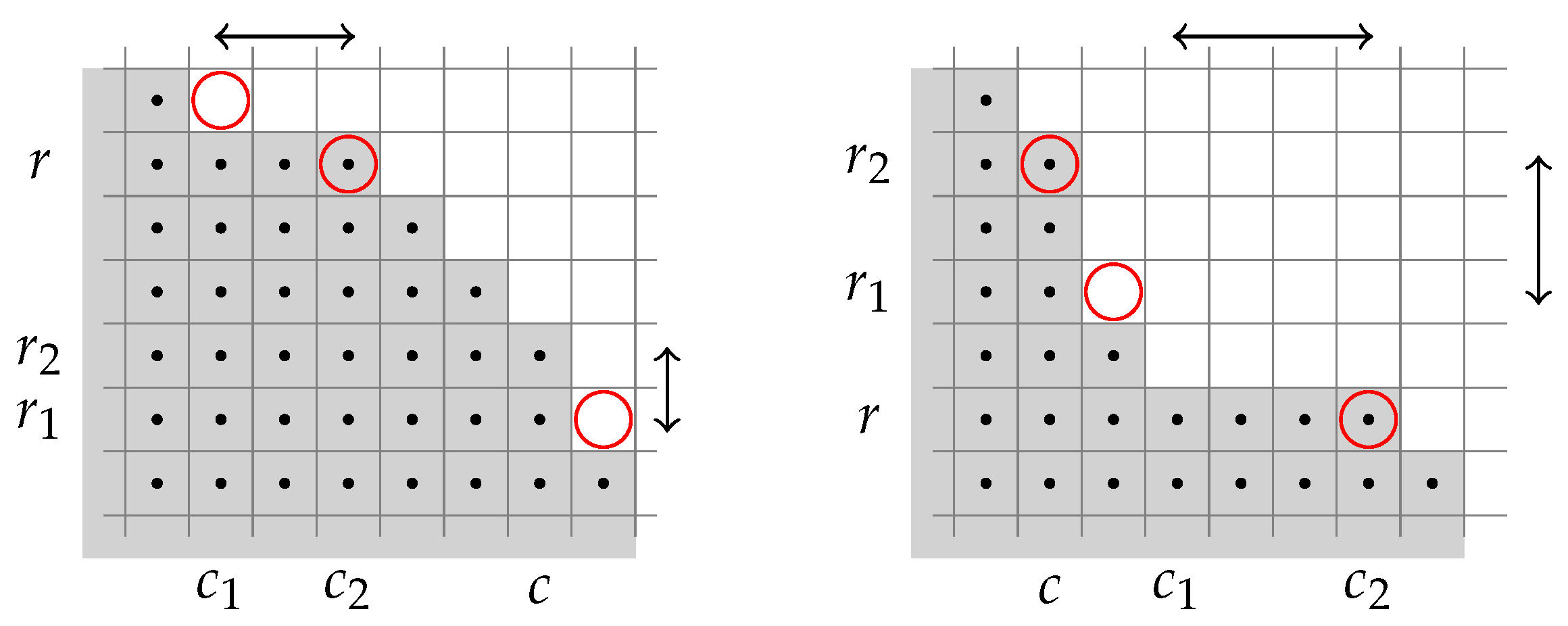
If $S^{\mathrm{col}}$ is not strictly decreasing, then the upper bound of S contains a horizontal segment length of at least 2. Similarly, if $S^{\mathrm{row}}$ is not strictly decreasing, then the right bound of S contains a vertical segment of length at least 2, see Figure 1. Take such a horizontal and a vertical segments whose distance is minimal. Let the horizontal segment be in row r between columns $c_1$ and $c_2$, and the vertical segment be in column c between rows $r_1$ and $r_2$. The horizontal and vertical segments are connected by (a possibly empty) diagonal staircase. Depending on which segment comes first, there are two possible arrangements as depicted on Figure 1.

In the first case $c_1<c_2<c$, and $r_1<r_2<r$; in the second case $c<c_1<c_2$ and $r<r_1<r_2$. Apply Lemma 11 to the marked points and observe that the modified downward closed sets are always subsets of $D_n$. In the first case

$${\displaystyle \frac{c_2-c_1}{(r+1)-r}}⩾1⩾{\displaystyle \frac{c+1-c_2}{r_1-r}},$$

(64)

and in the second case

$${\displaystyle \frac{(c+1)-c)}{r_1-r_2}}⩽1⩽{\displaystyle \frac{c_2-(c+1)}{r-r_1}}.$$

(65)

Therefore, by Lemma 11, ${\mathbf{v}}_S$ is superseded by the vectors generated by the indicated sets, proving the claim. □

By Corollary 2, the downward closed set corresponding to an extremal vertex is either a staircase with step heights 1 (when $S^{\mathrm{row}}$ is strictly decreasing), which we call horizontal, or the mirror image of such a staircase. The only configuration that belongs to both cases is the diagonal $D_n$. It will be more convenient to use the column-sequence $(c_0,c_1,\dots ,c_k)$ to represent horizontal staircases. Here $k⩾0$ is the length of the staircase, also denoted by $\mathrm{len}\left(S\right)$. The last column size (height) is necessarily $c_k=0$, and $c_i$ equals either $c_{i+1}$ or $c_{i+1}+1$ for every $0⩽i<k$. In the rest of this section, all staircases, if not mentioned otherwise, are horizontal ones.

Definition 5.

The staircase S is Positive-Negative-Positive (PNP)-reducible in $D_n$ if there are $i_1<i_2<i_3$ and $j_1>j_2>j_3$ such that $S_1=S+(i_1,j_1)$, $S_2=S-(i_2,j_2)$, and  $S_3=S+(i_3,j_3)$ are staircases in $D_n$ and ${\mathbf{v}}_S$ is superseded by $\{{\mathbf{v}}_{S_1},{\mathbf{v}}_{S_2},{\mathbf{v}}_{S_3}\}$. S is PNP-irreducible if it is not PNP-reducible.

Negative-Positive-Negative (NPN)-reducibility and NPN-irreducibility is defined analogously, using staircases $S-(i_1,j_1)$, $S+(i_2,j_2)$, and $S-(i_3,j_3)$, assuming that they are also subsets of $D_n$. S is irreducible in $D_n$ if it is both PNP- and NPN-irreducible. Finally, let ${\mathcal{S}}_n$ be the collection of the irreducible staircases that are subsets of $D_n$.

By the remark at the beginning of this section, by Lemma 11, and by Corollary 2, extremal vertices are generated by elements of ${\mathcal{S}}_n$ and by their mirror images. We describe an incremental algorithm that generates the elements of the collection ${\mathcal{S}}_n$.

A horizontal staircase S of length n can be recovered from a unique horizontal staircase $S^{\prime }$ of length $n-1$ as follows. If $S^{\prime }$ has the column sequence $(c_0^{\prime },c_1^{\prime },\dots ,c_{n-1}^{\prime })$, then S is defined by one of the column sequences

$$\begin{array}{ccccc}(c_0^{\prime },\hfill & c_1^{\prime },\hfill & \dots ,\hfill & c_{n-1}^{\prime },\hfill & 0) \mathrm{or}\hfill \\ (c_0^{\prime }+1,\hfill & c_1^{\prime }+1,\hfill & \dots ,\hfill & c_{n-1}^{\prime }+1,\hfill & 0),\hfill \end{array}$$

(66)

depending on whether the last two elements of the column sequence of S are equal.

Claim 6.

(i) 

Suppose S has length n. S is irreducible in $D_{n+1}$ if and only if it is irreducible in $D_m$ for any $m⩾n+1$.

(ii) 

If $\mathrm{len}\left(S\right)=n$ and S is irreducible in $D_n$, then $S^{\prime }$ is irreducible in $D_{n-1}$.

(iii) 

If $S\in {\mathcal{S}}_n$ but $S\notin {\mathcal{S}}_{n+1}$, then $\mathrm{len}\left(S\right)=n$ and S is PNP-reducible in $D_{n+1}$ with $i_3=n+1$ and $j_3=0$.

(iv) 

If $S^{\prime }\in {\mathcal{S}}_{n-1}$ and $S\notin {\mathcal{S}}_n$, then either S is NPN-reducible with $i_3=n$ and $j_3=0$, or it is PNP-reducible with $i_3=n-1$ and $j_3=1$.

Proof. 

(i) is immediate from the definition as the staircases $S\pm (i,j)$ must be subsets of $D_{n+1}$.

(ii) Assume $S^{\prime }$ is reducible in $D_{n-1}$ shown by the staircases $S_1^{\prime }$, $S_2^{\prime }$ and $S_3^{\prime }$. Since they are in $D_{n-1}$, they can be lifted back to $S_1$, $S_2$, $S_3$ in $D_n$. According to Lemma 11 these staircases witness the reducibility of S.

(iii) If S is reducible in $D_{n+1}$ but not in $D_n$, then $S+(i_3,j_3)$ is not in $D_n$, leading to the stated condition.

(iv) If S is reducible in $D_n$ while $S^{\prime }$ is not reducible in $D_{n-1}$, then the reduction must use $(i_3,j_3)$, which is in $D_n$ but not in $D_{n-1}$. If it is an NPN-reduction then it must use the newly added point $(n,0)$; in other cases the reduction can be shifted back to $S^{\prime }$. In the case of a PNP-reduction this additional point is $(n-1,1)$ (when extending the staircase by a column of height zero), or can be shifted back to $S^{\prime }$ again. □

Based on Claim 6, the incremental algorithm, sketched as Algorithm 1, generates all horizontal irreducible staircases. The PNP- and NPN-irreducibility can be checked based on Lemma 11. The last point $(i_3,j_3)$ is fixed, and the naïve implementation requires quadratic running time in $\mathrm{len}\left(S\right)$. With some simple bookkeeping it can be reduced to a backward scanning of the column sequence, resulting in linear running time.

Using the algorithm we have computed the complete set of irreducible staircases up to $n=60$. The number of new staircases that remained irreducible in each subsequent generation matches the sequence A103116 in the Encyclopedia of Integer Sequences [39]:

$${\mathrm{remains}}_n=\sum _{i⩽n}(n-i+1)\phi \left(i\right),$$

(67)

where $\phi$ is Euler’s totient function, which suggests that the connection is based on the number of different slopes determined by the lattice points in a rectangle. Proving the equivalence of these two sequences is an intriguing open problem.

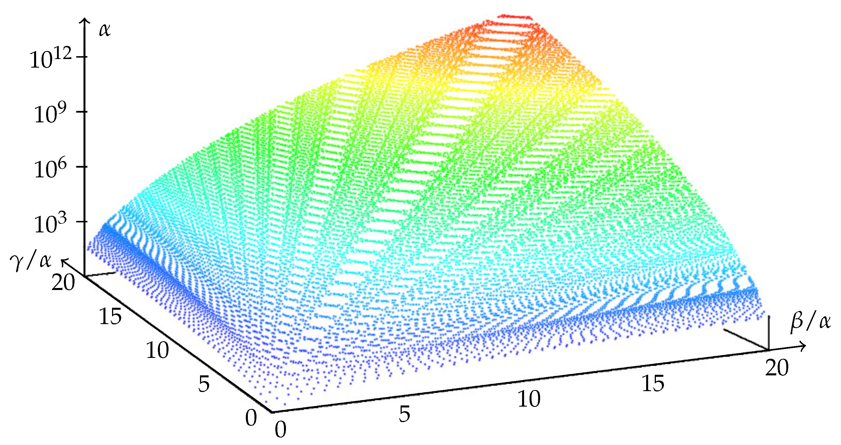
For better visualization, triplets $\langle {\alpha }_S,{\beta }_S,{\gamma }_S\rangle$ corresponding to these irreducible staircases are plotted as the three-dimensional points $\langle \beta /\alpha ,\gamma /\alpha ,\alpha \rangle$ using logarithmic scale for the third $\alpha$ coordinate. The plot in Figure 2 contains all 126,981 extremal triplets in the range $\beta ,\gamma ⩽20\alpha$. Some of the plotted triplets appear as late as generation $n=80$; later generations do not contribute to this part of the complete set. For comparison, some triplets in the 80-th generation have values larger than $2^{85}$.

Algorithm 1: Generating irreducible staircases

To explain the shape of the surface of extremal triplets plotted in Figure 2, we provide some heuristic reasoning. A consequence of Corollary 1 is that if the extremal triplet ${\mathbf{v}}_S$ is computed from the staircase S, then the slopes determined by the step edges $(i,j)\in S$ (namely, points of S where neither $(i+1,j)$ nor $(i,j+1)$ are in S) are almost equal. Consequently, on a large scale, extremal ${\mathbf{v}}_S$ vectors are generated by the set of lattice points in right-angled triangles defined by the inequality

$$S(a,b)=\{(x,y)\in \mathbb{N}\times \mathbb{N}:{\displaystyle \frac{x}{a}}+{\displaystyle \frac{y}{b}}⩽1\}$$

(68)

for some positive values of a and b. Since, by Lemma 5,

$$\begin{array}{cc}\hfill \sum _{i⩽x,j⩽y}\mathit{b}(i,j)& \approx \mathit{b}(x+1,y+1), \mathrm{and}\hfill \\ \hfill \sum _{i⩽x,j⩽y}i\mathit{b}(i,j)& \approx x\mathit{b}(x+1,y+1),\hfill \end{array}$$

the vector ${\mathbf{v}}_{S(a,b)}$ is well approximated by $\mathit{b}(x+1,y+1)\langle 1,x,y\rangle$, where $(x,y)\in S(a,b)$ is the point where $\mathit{b}(x+1,y+1)$ takes its maximal value. As the function $\mathit{b}(x,y)$ strictly increases in both coordinates, this maximum is taken on the boundary diagonal of the right-angled triangle $S(a,b)$ that has endpoints $(0,b)$ and $(a,0)$. Using the Stirling formula $n!\approx \sqrt{2\pi n}{(n/e)}^n$, we have

$$\mathit{b}(x,y)={\displaystyle \frac{(x+y)!}{x!y!}}\approx {\displaystyle \frac{1}{\sqrt{2\pi }}}{\displaystyle \frac{{(x+y)}^{x+y+1/2}}{x^{x+1/2}{y}^{y+1/2}}}.$$

(69)

Introducing $\phi \left(x\right)=(x+{\displaystyle \frac{1}{2}})\log x$, we see that the logarithm of $\mathit{b}(x,y)$ is well approximated by the function

$$\theta (x,y)=\phi (x+y)-\phi \left(x\right)-\phi \left(y\right)-\log \sqrt{2\pi }.$$

(70)

Using this approximation, the point $(u,v)$ is extremal in the triangle $S(a,b)$ if $(u,v)$ is on the boundary diagonal and $\theta (u+1,v+1)$ has zero derivative along this diagonal. For fixed u and v such a positive a and b exist just in case the partial derivatives ${\theta }_x$ and ${\theta }_y$ are positive at $(u+1,v+1)$. By inspection, this condition is satisfied for every $(u,v)$. Consequently, if $\langle \alpha ,\beta ,\gamma \rangle$ is an extremal triplet, then choosing $u=\beta /\alpha$, $v=\gamma /\alpha$, we expect

$$\log \alpha \approx \theta (u+1,v+1),$$

(71)

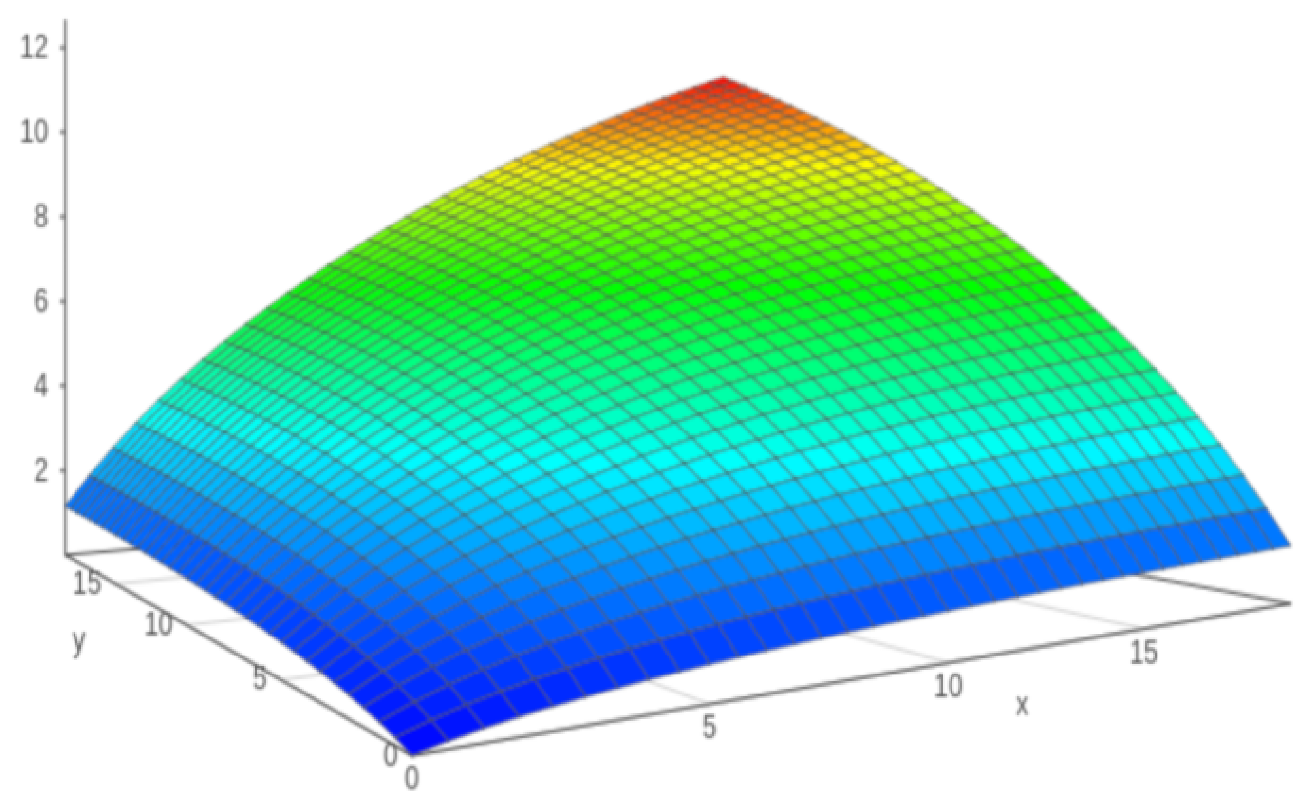
and, conversely, for each u, v, with the choice $\log \alpha =\theta (u+1,v+1)$, $\beta =u\alpha$, and $\gamma =v\alpha$, we expect the triplet $\langle \alpha ,\beta ,\gamma \rangle$ to be extremal. For comparison, Figure 3 plots these triplets over the same range that was used in Figure 2.

This approximation seems to slightly underestimate the real value of $\log \alpha$. For example, the extremal triplet obtained from the diagonal staircase $D_{n+1}$ is

$$\alpha =2^{n+1}-1,\beta =(n-1)2^n+1,\gamma =(n-1)2^n+1,$$

(72)

thus, $u=v=\beta /\alpha \approx (n-1)/2$, and $\log \alpha \approx (n+1)\log 2$. At the same time,

$$\theta (u+1,v+1)=(n+1)\log 2-\log \sqrt{n+1}+O\left(1\right).$$

(73)

Extremal triplets on the two edges of the surface are specified by the totally flat, stairless staircases. These triplets are

$$\alpha =n,\beta =n(n-1)/2,\gamma =0$$

(74)

on one axis, and $\beta$, $\gamma$ swapped on the other. In this case, the $(u,v)$ pair is $\left(\right(n-1)/2,0)$, and

$$\theta (u+1,v+1)=\log n+\left(1-\log \sqrt{8\pi }+O(1/n)\right),$$

(75)

which differs from the correct value by a constant only.

We have also looked at how the newly discovered entropy inequalities delimit the 5-variable entropy region. The triplet $\langle {\alpha }_S,{\beta }_S,{\gamma }_S\rangle$ yields the inequality

$$(a,b|z)+{\alpha }_S\left(\left[abcd\right]+\mathcal{Z}\right)+{\beta }_S\mathcal{C}+{\gamma }_S\mathcal{D}⩾0.$$

(76)

Since the closure of the 5-variable entropy region is a pointed convex cone, one can normalize it by assuming $(a,b|z)=1$. An equivalent view is to take the cross-section of $\overline{{\Gamma }_5^{\ast }}$ by this hyperplane. Consider the three-dimensional subspace spanned by the vectors

$$\begin{array}{lll}\hfill \mathbf{x}& \stackrel{\mathrm{def}}{=}\mathcal{C}\hfill & =(a,c|b)+(b,c\left|a\right),\hfill \\ \hfill \mathbf{y}& \stackrel{\mathrm{def}}{=}\mathcal{D}\hfill & =(a,d|b)+(b,d\left|a\right),\hfill \\ \hfill -\mathbf{z}& \stackrel{\mathrm{def}}{=}\left[abcd\right]+\mathcal{Z}\hfill & =\left[abcd\right]+(a,z|b)+(b,z\left|a\right);\hfill \end{array}$$

(77)

observe that $\mathbf{z}$ is negated. Normalize the five-variable entropic function f so that it satisfies $f(a,b|z)=1$, then project it to this subspace. Use the scalar products $\langle f·\mathbf{x},f·\mathbf{y},f·\mathbf{z}\rangle$ as the projection coordinates. This three-dimensional cross-section of the five-variable entropy region is

$$\Delta =\left\{\langle f·\mathbf{x},f·\mathbf{y},f·\mathbf{z}\rangle \in {\mathbb{R}}^3:f\in \overline{{\Gamma }_5^{\ast }} \mathrm{such} \mathrm{that} f(a,b|z)=1\right\}.$$

(78)

Clearly, points in $\Delta$ have non-negative x and y coordinates, while the z coordinate can take both positive and negative values. Since $\overline{{\Gamma }_5^{\ast }}$ is a closed convex cone, $\Delta$ is closed and convex. We concentrate on the part above the $xy$ plane:

$${\Delta }^{+}=\{\langle x,y,z\rangle \in \Delta :z⩾0\}.$$

(79)

Shannon inequalities provide no restriction whatsoever on ${\Delta }^{+}$ as any non-negative coordinate triplet can be realized by some polymatroid. To show this, define ${\mathit{r}}_I$ for any subset I of the ground set $abcdz$ as

$${\mathit{r}}_I:A\mapsto \left\{\begin{array}{cc}1\hfill & \mathrm{if} I\cap A\ne \varnothing ,\hfill \\ 0\hfill & \mathrm{otherwise}.\hfill \end{array}\right.$$

Let, moreover, ${\mathit{r}}^{\circ }$ be the function

$${\mathit{r}}^{\circ }:A\mapsto \left\{\begin{array}{cc}2\hfill & \mathrm{if} \left|A\right|=1,\hfill \\ 4\hfill & \mathrm{if} \left|A\right|⩾3, \mathrm{or}A \mathrm{is} \mathrm{one} \mathrm{of} cd,cz,dz,\hfill \\ 3\hfill & \mathrm{otherwise},\hfill \end{array}\right.$$

as A runs over the non-empty subsets of $abcdz$. Both ${\mathit{r}}_I$ and ${\mathit{r}}^{\circ }$ are extremal rays of ${\Gamma }_5$, so they are polymatroids. For arbitrary non-negative numbers $x, y, z$ the linear combination $f={\mathit{r}}_{abcd}+x{\mathit{r}}_{ac}+y{\mathit{r}}_{ad}+z{\mathit{r}}^{\circ }$ satisfies $f(a,b|z)=1$ and has coordinates $\langle x,y,z\rangle$, providing the required polymatroid.

Points of ${\Delta }^{+}$ with non-negative x and y coordinates and $z=0$ are realized by linear polymatroids; thus, the complete non-negative quadrant of the $xy$ plane is a part of ${\Delta }^{+}$. Our first non-Shannon inequality, generated by the triplet $S_{D_1}=\langle 1,0,0\rangle$, is

$$(a,b|z)+[abcd]+\mathcal{Z}⩾0.$$

(80)

This inequality immediately limits the region ${\Delta }^{+}$ to $z⩽1$; therefore, points in ${\Delta }^{+}$ have a height at most 1.

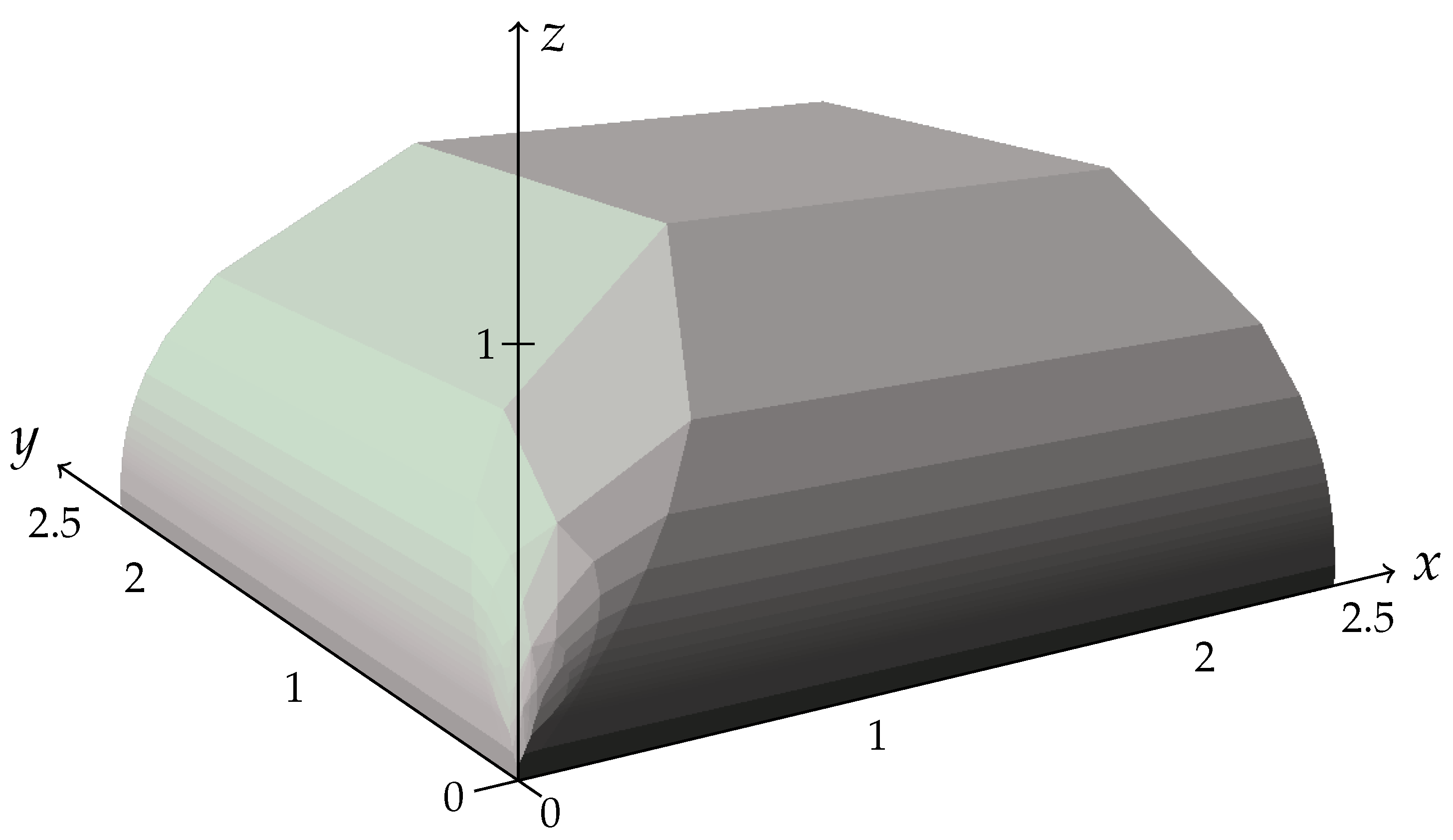
Other extremal triplets provide additional linear constraints. Figure 4 illustrates the delimited part of the non-negative octant as viewed from the origin, and cut at $x⩽2.5$ and at $y⩽2.5$. The pictured bound of ${\Delta }^{+}$ is extended to larger values of x and y. Along the x and y axes, this bound approaches the $xz$ and $yz$ coordinate planes as the functions $z=\sqrt{y}$ and $z=\sqrt{x}$, respectively. Along the $xy$ diagonal, the limiting behavior toward the z axis is similar to the entropy function $z=-(x+y)\log (x+y)$. The corner point of the plateau $z=1$ has coordinates $\langle 1,1,1\rangle$. The $\theta (u+1,v+1)$ estimate gives a smooth bound on ${\Delta }^{+}$, which is asymptotically tight along the x and y axes.

9. Conclusions

Structural properties of the entropy region of four or more variables are mostly unknown. This region is bounded by linear inequalities corresponding to the non-negativity of Shannon information measures. Finding additional entropy inequalities is, and remains, an intriguing open problem. Previous works on generating and applying such non-Shannon entropy inequalities focused mainly on the four-variable case [4,10,14,15], and only a few sporadic five-variable non-Shannon inequalities have been discovered [18]. This work provides infinitely many five-variable non-Shannon information inequalities by systematically exploring a special property of entropic vectors. Other works utilized the Copy Lemma, a method distilled from the original Zhang–Yeung construction by Dougherty et al. [14]. Our method is based on a different paradigm derived from the principle of maximum entropy and is a special case of the Maximum Entropy Method described in [20]. As proven in Lemma 1, the principle of maximum entropy implies that every entropic polymatroid has an $n,m$-copy, which is a polymatroidal extension with special properties as defined in Definition 1. In Claim 1, we have proved that polymatroids having $n,m$-copies form a polyhedral cone and hint at how its facets can be computed. Facet equations provide the potentially new non-Shannon entropy inequalities.

While the polyhedral computation presented in Claim 1 is numerically intractable even for small parameter values, the theoretical results of Section 4 allowed us to reduce this complexity significantly. Computational aspects of determining the facets of a high-dimensional cone are closely related to linear multi-objective optimization [22]. We have developed a specially tailored variant of Benson’s inner approximation algorithm [22,38], which takes advantage of the special properties of this enumeration problem. Computational results are reported in Section 5 for generations $n⩽9$. Numerical instability, originating from both the underlying LP solver and the polyhedral algorithm, prevented the completion of the computation for larger values of n.

Non-Shannon inequalities obtained from these computations are discussed in Section 6. Based on these experimental results, two infinite families of five-variable inequalities were defined. The first family in Theorem 1 is parametrized by downward closed subsets of non-negative lattice points. The second family in Theorem 2 has a single positive integer parameter. Inequalities in both families are proved to hold for polymatroids on five elements that have an n-copy; consequently, they are all valid entropy inequalities. It is conjectured that they cover all inequalities that can be obtained by the applied method. In other words, if a polymatroid on five elements satisfies all these inequalities, then it has an n-copy for all n. This conjecture is left as an open problem. The computational results confirmed this conjecture up to $n=9$.

Inequalities in the first family are investigated in Section 8 in more detail. They are specified by triplets $\langle {\alpha }_x,{\beta }_S,{\gamma }_S\rangle$ determined by downward closed sets S of nonnegative lattice points as discussed in Definition 4. Such a triplet is extremal if the corresponding inequality is not a consequence of other inequalities from the same family. Extremal triplets are determined by a special collection of downward closed sets called irreducible staircases. Based on the theoretical results in Corollary 2 and Claim 6, an incremental algorithm, sketched as Algorithm 1, was used to generate irreducible staircases up to generation 60. The converse implication, valid for the computed cases, that triplets generated by irreducible staircases are extremal, is left as an open problem. Triplets (${\alpha }_S,{\beta }_S,{\gamma }_S\rangle$ in the range ${\beta }_S,{\gamma }_S⩽20{\alpha }_S$, generated by irreducible staircases, are plotted in Figure 2. The number of new irreducible staircases that remained irreducible in the subsequent generation matches the sequence A103116 in the Encyclopedia of Integer Sequences [39]. It is an interesting open problem to prove the equality of these sequences.

To illustrate how the newly discovered entropy inequalities delimit the five-variable entropy region, entropy vectors were normalized to satisfy $(a,b|z)=1$ and projected onto a three-dimensional subspace. Part of the projection in the non-negative octant is denoted by ${\Delta }^{+}$. The Shannon inequalities do not provide any restriction on this part. Figure 4 illustrates the bounds implied by the new inequalities. While the non-negative quadrant of the $xy$ plane is known to be part of ${\Delta }^{+}$, and that it also contains points above that plane, it is an intriguing open problem whether our bound is, at least asymptotically, tight around the x and y axes. Showing that our bound is asymptotically tight at the zero point would amount to settling the long-standing open problem of whether the entropic region is semi-algebraic.