


Abstract
A representative cluster-based model of the batch process of ethanol production by Kluyveromyces sp. is proposed. Experimental data from fermentation processes of 17 different strains of K. marxianus are used; each of them potentially exhibits different metabolic and kinetic behavior. Three algorithms for clustering are applied. Two modifications of Principal Component Analysis (PCA)—hierarchical clustering and k-means clustering; and InterCriteria Analysis (ICrA) are used to simplify a large dataset into a smaller set while preserving as much information as possible. The experimental data are organized into two main clusters. As a result, the most representative fermentation processes are identified. For each of the fermentation processes in the clusters, structural and parameter identification are performed. Four different structures describing the specific substrate (glucose) consumption rate are applied. The best structure is used to derive the representative model using the data from the first cluster. Verification of the derived model is performed using experimental data of the second cluster. Model parameter identification is performed by applying an evolutionary optimization algorithm.
1. Introduction
Ethanol fermentation is a key biotechnological process widely used in the production of biofuels, alcoholic beverages, and industrial solvents. Yeasts have a long tradition of application in biotechnology and a more recent history of use as model organisms for fundamental research in biochemistry, metabolism, genetics, and cell biology [1]. The application of modern microbiological and molecular approaches has resulted in renewed focus on the biology and industrial potential of the yeasts. Among the various microorganisms employed for ethanol production, Kluyveromyces marxianus is a prominent candidate for ethanol production due to its fast growth rate and inherent thermotolerance. Furthermore, its ability to directly convert diverse sugars like lactose, xylose, and inulin under aerobic conditions greatly expands its utility in processing various biomass feedstocks [2]. Despite the importance of these traits and extensive exploitation by the biotechnology sector, fundamental research with K. marxianus is just emerging. The versatility of this microorganism makes it particularly attractive for second-generation bioethanol production, for example—from cellulosic biomass, which is a renewable and abundant resource [3]. However, regardless of these benefits, a notable limitation of K. marxianus is its relatively low ethanol tolerance, which can impede its performance in high-ethanol-concentration fermentations [4]. However, adaptive laboratory evolution studies have shown that exposing K. marxianus to increasing ethanol concentrations can enhance its tolerance [5].
While existing models offer a solid foundation for understanding ethanol fermentation by K. marxianus, they present certain limitations. Specifically, in references [6,7,8], the models assume homogeneous behavior across strains, which may not adequately capture the pronounced biological heterogeneity observed among different K. marxianus strains. Additionally, the influence of dynamic environmental factors—such as temperature fluctuations, substrate inhibition at high concentrations, and stress responses towards physicochemical and biological conditions—is often simplified or omitted.
In Ref. [6], a kinetic model of batch production of ethanol as a by-product of the cheese or dairy industry (industrial waste—whey), using lactose-containing raw material, is proposed. The classical Monod model is used to describe the specific growth rate. This process presents a novel approach to secure both energy and the environment and is the subject of several other studies. The same model is used to describe batch and fed-batch processes, carried out under the same physicochemical conditions, and to compare the operation modes of the fermentation system for ethanol production from whey using K. marxianus [7]. In Ref. [8], the model for fed-batch fermentations with different temperatures as initial conditions for optimization purposes is investigated.
The inherent non-linear and non-stationary dynamics of fermentation processes render their precise mathematical modelling exceptionally difficult [9,10]. To address the challenges of structure and parameter identification in complex biotechnological processes, metaheuristic optimization algorithms represent a commonly adopted approach. Metaheuristics are strategic frameworks designed to guide solution searches beyond the limitations of traditional deterministic methods, such as the Levenberg-Marquardt algorithm. These metaheuristic approaches are less sensitive to initial conditions and better equipped to avoid local minima when modeling complex fermentation processes with inhibition terms and correlated parameters. The metaheuristic algorithms are characterized by two essential components:
- Diversification: The generation of a wide range of candidate solutions to explore the parameter space broadly in search of a global optimum.
- Intensification: The focused search within promising regions known to contain high-quality solutions (local optimum).
For decades, metaheuristics have proven highly effective across various fields for tackling complex problems [11], establishing themselves as among the most potent strategies for optimization [12]. Among metaheuristic algorithms, evolutionary algorithms are particularly effective for the inherently non-linear, constrained, and multi-objective characteristics of bioprocess modelling and model parameter identification. To enhance the optimization’s reliability and avoid stagnation at local optima, a multi-start strategy is employed, which improves the robustness of the algorithm and the likelihood of identifying high-quality solutions [13,14].
A key step before model building is data preprocessing. As a statistical tool for multivariate analysis, Principal Component Analysis (PCA) is intended to consolidate numerous variables into a new, smaller collection of data called components [15]. PCA provides a concise overview of a dataset. It is highly effective in recognizing patterns in data: outliers, trends, groups, relationships, etc. [16]. The broad utility of this method is evidenced by its extensive use in fields ranging from clustering [17] to decision-making [18] and noise reduction [19].
InterCriteria Analysis (ICrA) [20] is another possible technique for dataset clustering. ICrA is based on the theory of intuitionistic fuzzy sets (IFS) [21,22] and utilizes the apparatus of index matrices (IM) [23]. Applying ICrA yields an IM of intuitionistic fuzzy pairs (IFP) [22]. Although ICrA is not a widely known approach, it offers certain advantages over established statistical methods [24,25,26,27].
In [28], the InterCriteria Analysis (ICrA) method has been used to evaluate and select growth rate models for cultivation by the strain K. marxianus var. lactis MC 5. Ten unstructured models have been initially considered to model the cell growth kinetics. The application of the ICrA revealed numerous correlations among the investigated models. The models were subsequently reduced to a growth rate dependent only on lactose and a growth rate dependent only on oxygen. The use of ICrA permitted the investigation of various combinations of models for lactose and oxygen. In [29], a mathematical model of a batch fermentation of the K. marxianus strain has been investigated. The model includes bioreactor mass transfer of oxygen concentration in the gas phase (GP) and the liquid phase (LP). A dispersion model of the GP and perfect mixing in the LP is assumed. Nine models of the specific growth rate and the specific oxygen consumption rate were investigated. For parameter identification, the largest observed error was employed as the objective function across all experiments. This approach represents a special case of multi-objective parameter identification, effectively transforming the problem into a min-max optimization. Furthermore, the parameters used in the models are often derived empirically, a fact that can be particularly limiting and prevents their use in developing various monitoring and control algorithms.
Despite the substantial body of modelling studies on ethanol fermentation by K. marxianus, several important aspects remain insufficiently addressed. Existing works typically focus on individual strains or small datasets and implicitly assume homogeneous kinetic behavior [30,31], which limits their ability to represent the pronounced strain-to-strain variability observed in experimental practice. Furthermore, model structures and parameters are often derived empirically for specific experiments, restricting their general applicability and usefulness for process monitoring, optimization, and control.
In this study, we address these limitations by proposing a systematic framework for the development of a representative cluster-based dynamic model of ethanol fermentation that is representative of a class of K. marxianus strains. The key novelty lies in the combined application of multivariate data analysis techniques—Principal Component Analysis and InterCriteria Analysis—to objectively cluster experimental datasets and identify representative fermentation behaviors, followed by structure and parameter identification based on averaged, cluster-specific experimental profiles. This approach enables the selection of an optimal kinetic structure using statistical criteria and the derivation of robust model parameters using evolutionary optimization.
From a scientific perspective, the proposed methodology provides a principled way to reconcile biological heterogeneity with model generalization. This approach preserves mechanistic interpretability while extending applicability across multiple strains. From a practical standpoint, the resulting mathematical model offers a reliable foundation for the development of monitoring, optimization, and control strategies in industrial ethanol fermentation processes. Such a foundation is essential where strain variability and limited experimental reproducibility are inherent challenges.
Using experimental data of 17 different strains of K. marxianus, each potentially exhibiting distinct metabolic and kinetic behaviors, the ethanol fermentation process is modelled. The primary goal is to develop a cluster-based representative model that captures the typical dynamics of the studied fermentation processes under the considered conditions.
The mathematical model is derived based on the General Dynamic Model (GDM) approach [4]. The GDM approach has been successfully employed in a number of studies related to the modelling, monitoring, and control of biotechnological processes [32,33,34]. The experimental datasets from all K. marxianus strains are processed employing PCA and ICrA.
Moreover, the idea of searching for the most suitable kinetic structure for the specific substrate consumption rate with inhibition will be realized with glucose as the primary substrate instead of lactose. For the model structure and parameter identification, a metaheuristic optimization strategy is applied [10,35]. Further, the developed representative cluster-based model is verified using an independent dataset.
The paper is organized as follows. Section 2 describes the considered fermentation process and provides a detailed description of the metaheuristic method used—an Evolutionary algorithm (EA). Section 3 presents the mathematical modelling approach—GDM. Section 4 details the application of two modifications of PCA (hierarchical clustering and k-means clustering) and ICrA to simplify a large dataset into a smaller one while preserving as much information as possible. As a result, the most representative fermentations are identified. Section 5 presents and discusses the obtained results, and Section 6 concludes the research.
2. Materials and Methods
2.1. Microorganism and Fermentation Process Conditions
Experimental data were obtained from batch alcoholic fermentation by K. marxianus. Seventeen strains with distinct genetic profiles were investigated to study growth kinetics, glucose consumption, and ethanol production. The codification and origin of the studied K. marxianus karyotypes are reported in [3,36]: fifteen strains were isolated from agave fermentations for mezcal production in different regions of Mexico, and two reference strains were included (CBS6556, isolated from pozol in Mexico, and CBS397, isolated from yoghurt in The Netherlands).
All fermentations were performed under the same operating protocol across strains as described in [3]. The chemically defined medium had identical composition in all runs, with glucose initially set to 20 g/L [37]. Plates with the same medium supplemented with 20% agar were used only for strain conservation at 4 °C [37]. Fermentations were conducted in duplicate for each strain with hourly sampling. Biomass was quantified by OD600 (converted to g/L via calibration), while glucose and ethanol were measured by HPLC under the conditions reported in [3].
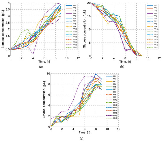
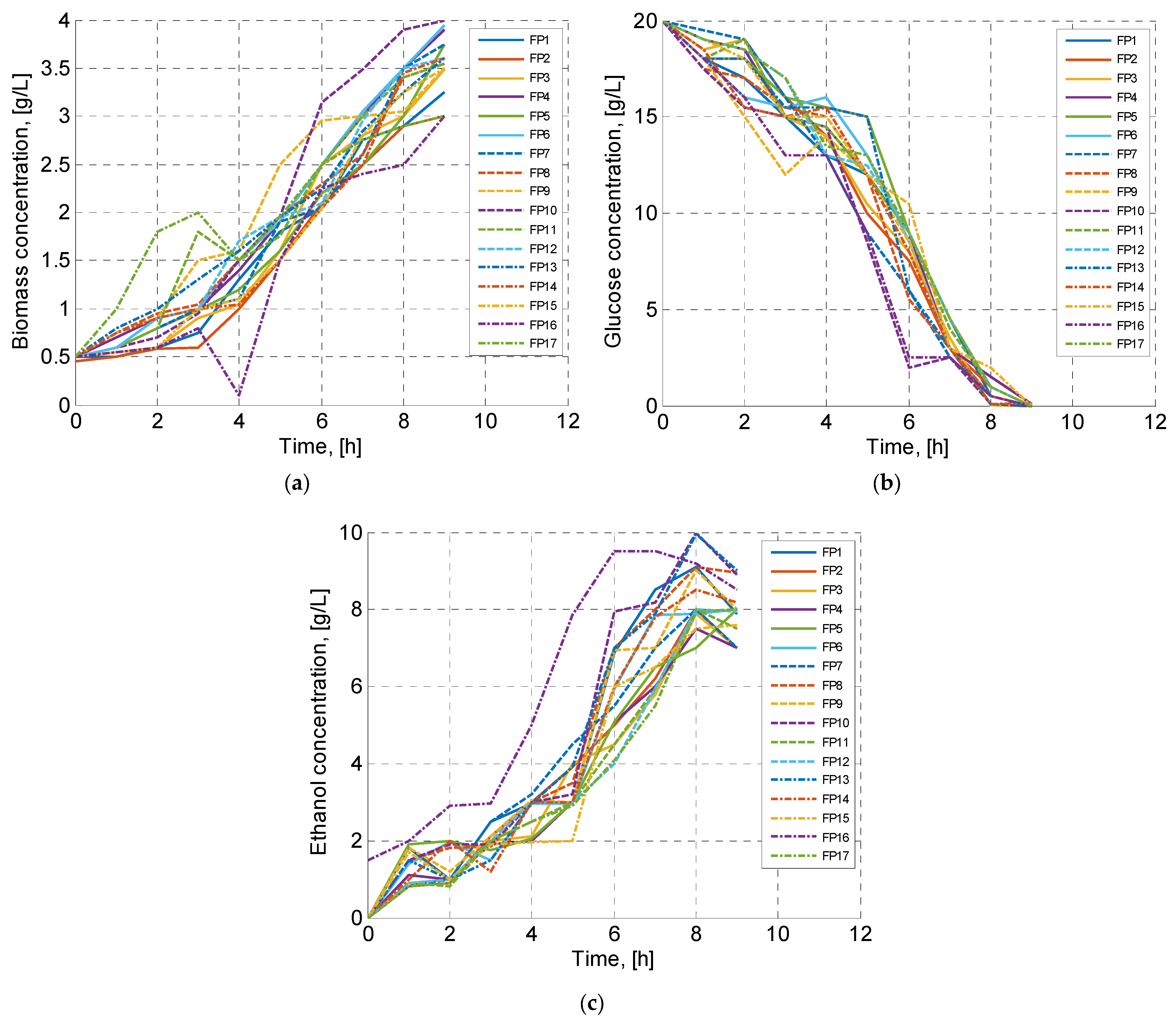
The fermentation processes operated in batch mode (closed system), i.e., yeast cultivation occurred in a fixed-volume medium containing the required nutrients. Figure 1 presents the concentration profiles of biomass, glucose, and ethanol for the 17 strains.
Figure 1.
Time profiles of process variables during batch alcoholic fermentation by 17 K. marxianus strains (17 fermentation processes (FP)): (a) glucose concentration, (b) biomass concentration, and (c) ethanol concentration (0–9 h).
Despite identical experimental conditions, the profiles reveal clear strain-to-strain differences: glucose depletion is broadly similar across datasets, whereas biomass growth and ethanol accumulation show more pronounced variability in rates, peak levels, and timing. This qualitative variability motivates the subsequent multivariate clustering and representative (cluster-based) model development.
2.2. Evolutionary Algorithm Background
The inherent non-linear, non-stationary, and strain-dependent nature of batch fermentation processes makes reliable structure and parameter identification particularly challenging. The considered models include inhibition effects, strongly coupled state variables, and parameters that are often correlated, which may lead to multiple local minima and identifiability issues when classical gradient-based optimization methods are applied. These difficulties are further amplified by experimental variability.
To address these challenges, an evolutionary optimization algorithm is employed for model parameter identification. Evolutionary algorithms are well-suited to this problem class due to their derivative-free nature, robustness to noisy objective functions, and ability to explore complex, multi-modal search spaces. In the present study, a multi-start evolutionary strategy is used to reduce sensitivity to initial parameter guesses and to improve convergence reliability across different kinetic structures. This approach enables consistent parameter estimation and objective comparison of competing model structures using statistical criteria, supporting the derivation of a robust fermentation model.
A comprehensive investigation was conducted into various model structures for the specific glucose consumption rate to identify the most representative kinetic structure. Additionally, a comparison was made between the results of the proposed model and those presented in the literature.
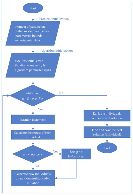
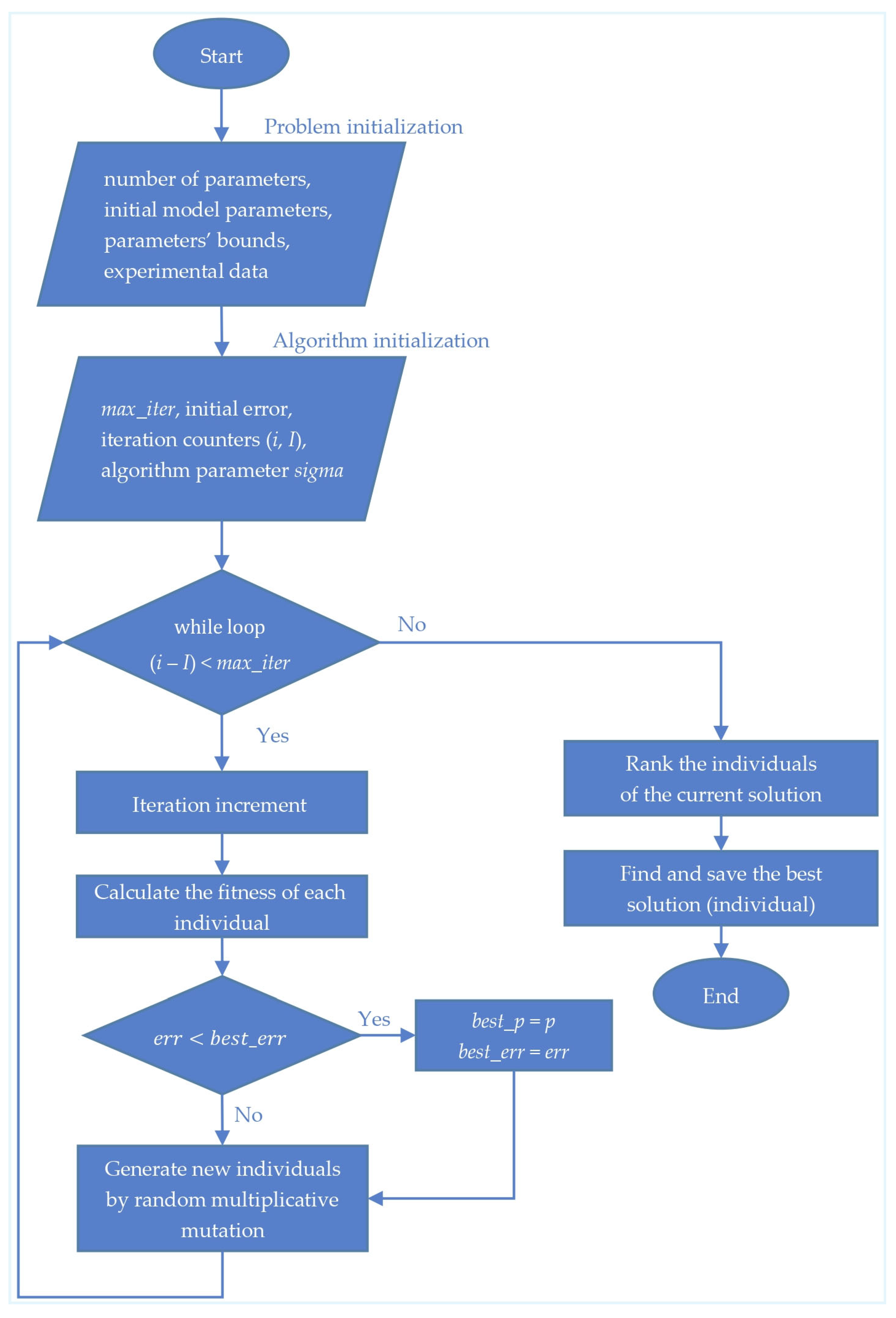
The flowchart of the applied EA is presented in Figure 2. The Algorithm 1 operates via the following steps:
| Algorithm 1 Evolutionary algorithm |
|
Figure 2.
Flowchart of the Evolutionary algorithm applied to model parameter identification.
Initially, the first parental population is generated. This population consists of n candidate solutions, where each solution is a set of model parameters for the optimization problem. The initial values for this generation are selected based on preliminary expert knowledge and are constrained to lie within physiologically possible intervals. Subsequently, the fitness functions (errors) are calculated to evaluate the performance of each candidate solution (i.e., the parameter estimates). The fitness function serves to quantify the goodness-of-fit of the solution to the optimization objective, considering both the model-data concordance and the adherence to the physiologically possible parameter bounds. If the stopping criterion is not met, new candidate parameters are generated with random multiplicative mutation, and the corresponding fitness functions are calculated. The process iteratively loops until the stopping criterion is met (specifically, the exhaustion of the maximum preset number of iterations). The EA then terminates, and the best model parameter values corresponding to the lowest accumulated error are presented as an optimal solution.
The objective function used for parameter identification is defined as the residual sum of squares (RSS) between the experimental measurements and the corresponding model predictions. For a given parameter vector , the RSS is computed as:
where and denote the experimental and model-predicted values, respectively, of the -th process variable at sampling time ; is the number of measured variables (biomass, glucose, and ethanol), and is the total number of experimental data points per variable.
The optimization problem consists of finding the parameter vector that minimizes subject to physiologically plausible parameter bounds.
All variables are treated with equal weighting to avoid introducing subjective bias and to allow objective comparison of competing model structures using statistical criteria.
The selected evolutionary strategy reflects the relatively low-dimensional parameter space and the emphasis on robustness rather than population diversity. Although a single-solution elitist evolution is employed, robustness against local minima is enhanced through a multi-start initialization scheme.
The MATLAB (v2019) environment was employed to implement the evolutionary algorithm, conduct all numerical experiments, and generate the graphical results.
The EA key parameters are specified in Table 1.
Table 1.
Key parameters of EA.
3. Mathematical Modelling Approach
The model development is founded on the principle of the GDM approach, which is specifically designed to address challenges associated with biotechnological systems, such as pronounced non-linear and non-stationary dynamics and the limited reproducibility of experimental data. The GDM approach represents the biotechnological process by a system of mass-balance equations derived from a set of key metabolic reactions.
The developed here mathematical models are formulated based on the following modelling assumptions [9]: (i) perfect mixing (spatially uniform concentrations of biomass, glucose, and ethanol); (ii) constant working volume and no inflow/outflow during the batch; (iii) yield coefficients – are constant lumped parameters over the considered time window; and (iv) the maintenance consumption term is neglected to keep the model simple and identifiable from the available data.
In this specific case, batch alcoholic fermentation with K. marxianus is described by two principal glucose-utilization pathways. The first reaction is oxidative growth of biomass on glucose (Equation (2)). The second reaction represents fermentative growth on glucose coupled with ethanol formation (Equation (3)). A third pathway—biomass growth on ethanol (ethanol reassimilation)—may occur after exhaustion of the primary substrate. Because ethanol is the target product, this pathway is undesirable for efficient bioproduction and is not included in the present model. Moreover, within the time window considered for model identification, the experimental ethanol profiles do not show a systematic decrease that would indicate net ethanol consumption; therefore, introducing an ethanol-consumption term would add complexity without being supported by the available observations.
The following core biotechnological reaction scheme is utilized for the development of models:
- Oxidative growth (biomass production):
- 2.
- Fermentative growth (biomass and ethanol production):
Biomass denotes cell biomass concentration (dry cell weight, g/L) inferred from OD600 calibration; it represents cellular material only and does not include substrate or product .
The mathematical model, derived from the reaction schemes in Equations (2) and (3), is presented in matrix form as follows:
Alternatively, the model can be written as a system of three ordinary differential equations:
where
and are the pathway-specific kinetic terms for the specific glucose consumption rates associated with oxidative and fermentative growth, respectively and is the specific glucose consumption rate for the oxidative and fermentative growth of the biomass.
Further, in Section 4, four competing kinetic models for , namely Monod [38], Galvanauskas et al. [39], Cockshott and Bogle [40], and Alba and Calvo [41], are investigated.
4. Data Analysis Based on PCA and ICrA
To select the most representative experimental data from the 17 available datasets, two methods for cluster analysis are applied—PCA, utilizing two different modifications (hierarchical clustering and k-means clustering), and ICrA.
PCA is a widely utilized dimensionality reduction technique that transforms a large set of correlated variables into a smaller set of uncorrelated variables, called principal components (PCs), which retain the maximum possible variance present in the original dataset. These PCs are constructed as linear combinations of the initial variables. The procedure ensures that the first principal component accounts for the largest possible variance, with subsequent components accounting for the maximal remaining variance. By organizing this information, PCA allows for the reduction of data dimensionality without significant information loss, by discarding components contributing minimally to the total variance and considering the remaining components as new variables.
In the present work, PCA is applied to reduce the number of experimental datasets. The original variables in the PCA are the time-series profiles of biomass, glucose, and ethanol concentrations from 17 independent fermentation processes. PCA enables the identification of kinetically similar datasets, which are grouped into clusters and subsequently represented by two generalized (cluster-averaged) experimental datasets used for model identification and verification.
To evaluate the performance of the clustering methods, the Silhouette value is calculated. As an unsupervised method, it does not require a training set to assess clustering quality. The Silhouette value is defined as [42,43]:
where is an element in cluster , is the average distance of to all other elements of the cluster , and , among all clusters . is the average distance from to all points in the cluster for .
ICrA is a decision-support method that yields an index matrix for IFP. Each IFP estimates the degrees of “agreement” (consonance) and “disagreement” (dissonance) between every two criteria (datasets). When comparing two criteria, the degree of “agreement” () is typically determined as the number of matching components of the respective vectors. Conversely, the degree of “disagreement” () is typically defined as the number of components with opposing signs in the two vectors. From the computation methodology, it follows that = and = . The IFP is an ordered pair of real non-negative numbers such that . The difference is considered the degree of “uncertainty” [20].
Although PCA is an effective and widely used tool for dimensionality reduction and visualization of multivariate datasets, its application alone is not sufficient for fully characterizing the complex, strain-specific differences observed in fermentation processes. PCA primarily captures directions of maximum variance in the data and emphasizes global trends; however, it may obscure subtle but biologically relevant differences between datasets, particularly when multiple process variables exhibit heterogeneous sensitivities or when clusters overlap in the reduced feature space.
To complement PCA, ICrA is employed as a relational, criterion-based method that explicitly evaluates the degrees of “agreement” and “disagreement” between experimental datasets for each process variable. Unlike PCA, ICrA does not rely on variance maximization or linear transformations, but instead provides a direct measure of similarity and dissimilarity between fermentation processes, enabling the identification of outliers and strain-specific deviations that may not be apparent in PCA projections.
The joint use of PCA and ICrA therefore provides a more robust and informative clustering framework: PCA offers an initial, variance-based grouping and visualization of the data, while ICrA refines this grouping by revealing hidden relationships and confirming or rejecting cluster assignments based on pairwise comparisons. This combined approach ensures that the selected representative fermentation datasets are both statistically coherent and biologically meaningful, which is essential for the subsequent derivation of a representative process model.
As a first step, hierarchical clustering and k-means clustering are applied to experimental datasets comprising the time profiles of biomass, glucose, and ethanol. Based on preliminary expert assessment, the datasets were organized into three clusters.
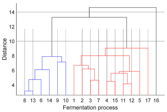
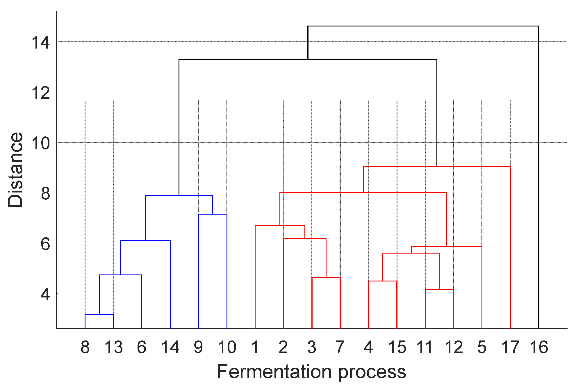
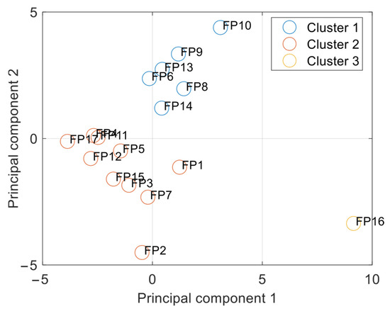
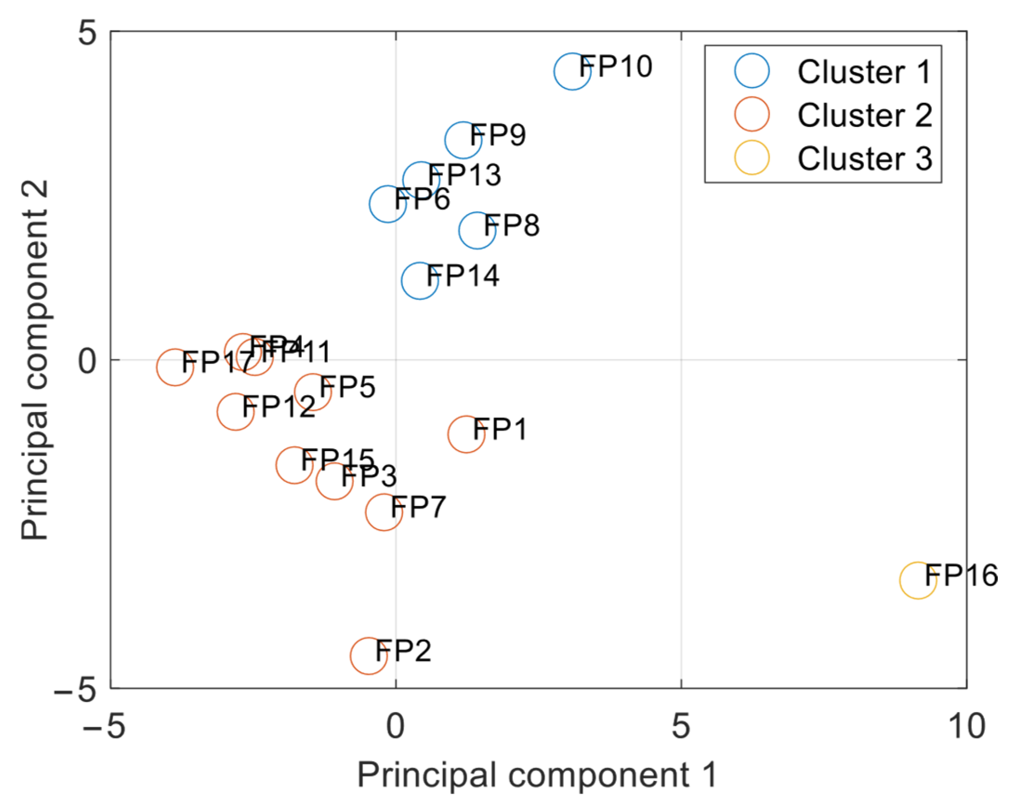
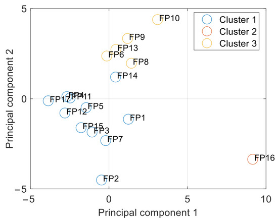
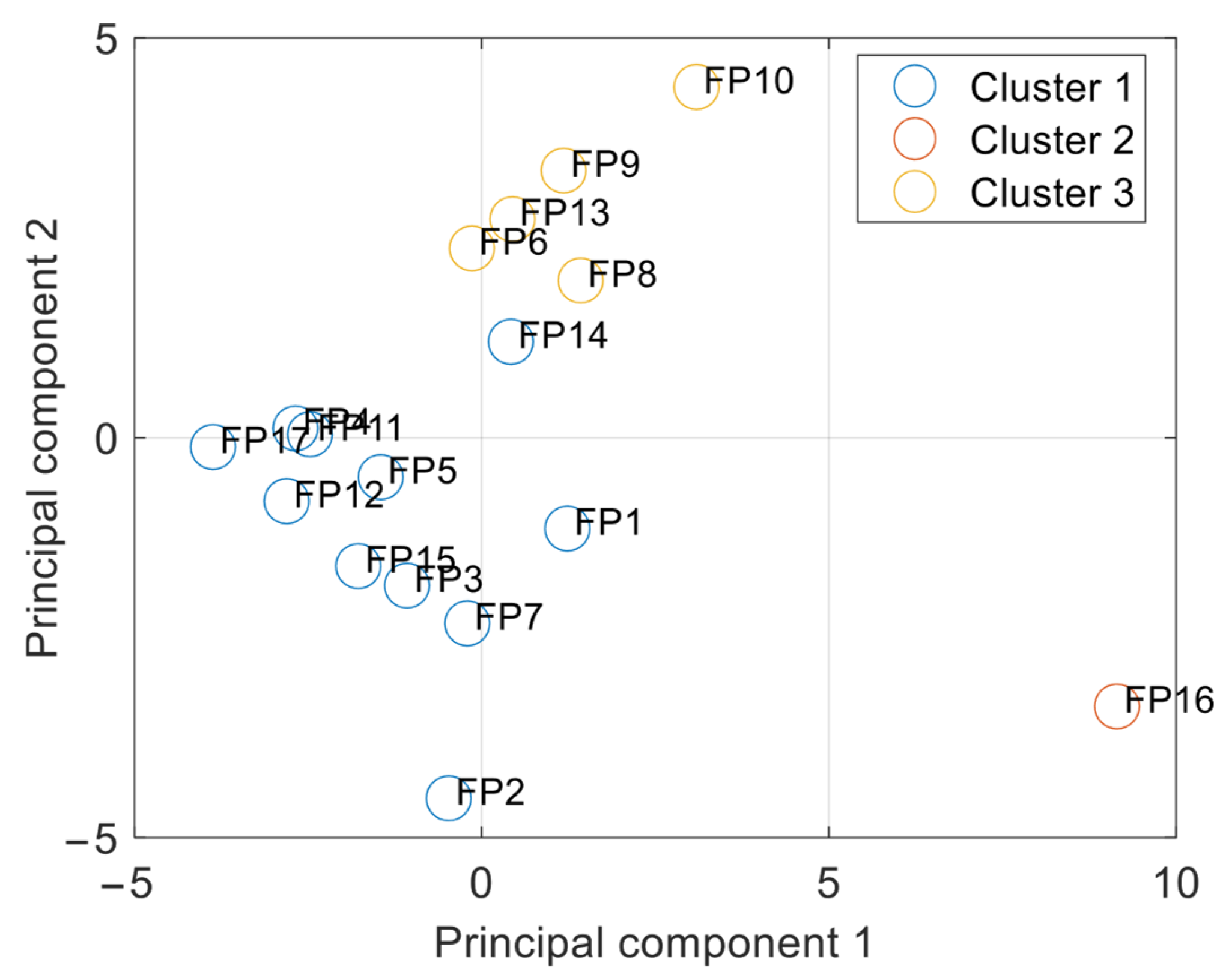
The results are summarized in Table 2, where FPi denotes the fermentation process of strain i of K. marxianus (e.g., FP6 signifies the fermentation process of strain 6). To visualize the results of hierarchical clustering, a tree-like diagram that shows the hierarchical relationships between FPs is presented in Figure 3. Figure 4 and Figure 5 present graphical output of the hierarchical and k-means clustering.
Table 2.
Results of PCA on the 17 fermentation processes datasets.
Figure 3.
Dendrogram of PCA—hierarchical clustering: blue—Cluster 1; red—Cluster 2, black—Cluster 3 (only FP16).
Figure 4.
Hierarchical clustering—resulting three fermentation processes clusters.
Figure 5.
k-means clustering—resulting three fermentation processes clusters.
The clustering results obtained from the two methods are similar, with the exception of FP14 (marked in bold). Both methods classify FP14 into different clusters. This discrepancy likely arose because the distance of FP14 to both Cluster 1 and Cluster 2 was approximately equidistant, leading to its random assignment.
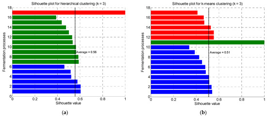
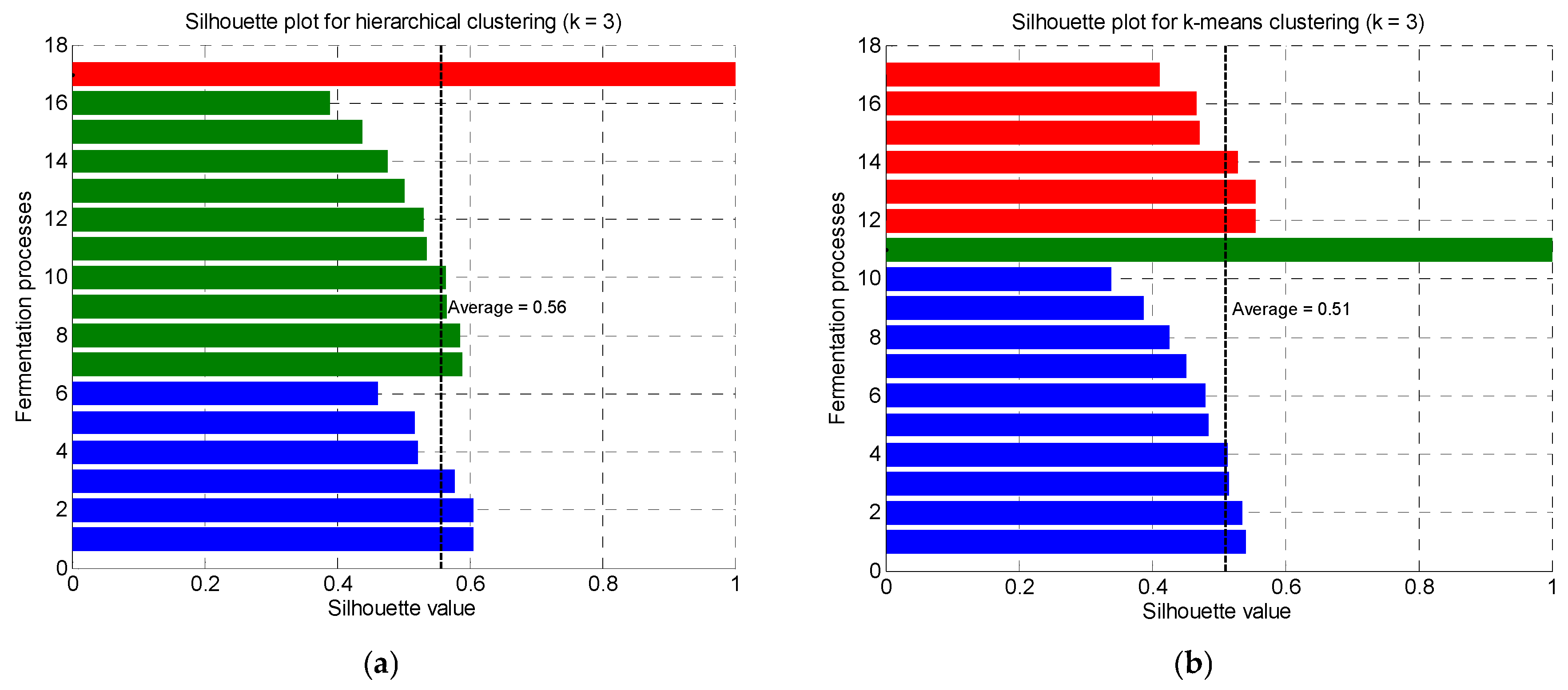
The selection of k = 3 (three clusters) was evaluated using silhouette analysis applied to the standardized, flattened fermentation datasets. The observed results, Silhouette values, calculated based on Equation (10), are presented in Figure 6.
Figure 6.
Silhouette plot: Silhouette values calculated for evaluation of (a) hierarchical clustering; (b) k-means clustering.
The obtained average silhouette value (0.535) indicates good cluster separation, which is consistent with the expected overlap of strain-dependent fermentation behaviors in biological systems. Importantly, one cluster exhibits a silhouette value close to unity, indicating a clearly distinct fermentation profile, while the remaining two clusters show high positive silhouette values, reflecting overlapping, coherent kinetic behaviors.
These results quantitatively support the choice of three clusters by confirming the presence of one isolated behavioral group and two broader, biologically related clusters. Increasing or decreasing the number of clusters was found to either merge distinct behaviors or fragment overlapping groups, reducing both interpretability and suitability for subsequent mathematical model derivation.
Detailed analysis of the experimental data profiles and PCA results revealed the following key characteristics:
- FP1: Exhibits robust growth, near-complete glucose consumption (final concentration near 0 g/L), and effective ethanol production (peak at 9.10 g/L). Represents a relatively efficient process.
- FP2 to FP4, FP15, FP17: Show good growth and glucose consumption, but exhibit moderate ethanol yields (peaks ranging from 7.50 g/L to 8.00 g/L).
- FP5 to FP7, FP11, FP12: Demonstrate consistent performance with good growth, complete glucose consumption, and good ethanol yields (peaks around 8.00 g/L).
- FP8 and FP9: Exhibit high-efficiency performance with high ethanol yields (peaks at 9.10 g/L and 9.00 g/L, respectively, with FP9 having a slight glucose residue).
- FP10 and FP13: Represent the highest performing processes, showing strong growth and very high ethanol titers (peaks at 10.00 g/L and 9.95 g/L, respectively).
- FP16: Presents significant kinetic anomalies. The initial ethanol concentration is 1.50 g/L (non-zero), and the biomass profile is erratic (e.g., 0.10 g/L at time point 5, followed by recovery). Despite high final ethanol (peak at 9.50 g/L), the discrepant initial conditions and dynamic behavior classify this dataset as an outlier.
In conclusion, the FP16 dataset is deemed unreliable for inclusion in representative model development.
In the subsequent step, the datasets are processed using ICrA. Based on the IMs (IM1, IM2, and IM3) derived from the biomass, glucose, and ethanol concentration profiles, all relations between datasets are evaluated by ICrA. The form of the input IMs and the obtained ICrA results are presented in Appendix A.
The performed ICrA reveals several critical insights:
- Glucose dataset: All fermentations are kinetically proximal with respect to glucose consumption profiles. FP14 shows only minor dissimilarities to FP2, FP3, FP10, and FP11.
- Biomass dataset: FP17 and FP16 are completely different from all other strains, and from each other, concerning the biomass growth kinetics.
- Ethanol dataset: FP16 is substantially different from the rest of the strains. FP1 exhibits noticeable differences from FP5, FP6, FP14, FP16 and FP17, while FP5 shows different behavior from FP7, FP8, FP9, FP12, FP13, FP15 and FP16.
It can be concluded that FP16 and FP17 are not appropriate for use in further investigation. Datasets FP16 and FP17 were excluded from the model development based on three predefined criteria: (i) significant deviation from initial batch conditions (e.g., non-zero initial ethanol in FP16), (ii) erratic biomass profiles that suggest experimental measurement noise rather than biological kinetics, and (iii) high dissonance () in ICrA results. While this exclusion focuses the model on the ‘consensus’ behavior of K. marxianus, it reduces potential bias from non-representative metabolic failures, ensuring the resulting representative model is optimized for predictable industrial production scenarios.
The analysis confirms that the most sensitive variables are ethanol and biomass. The biomass growth and ethanol production are strain-specific, whereas glucose is consumed in a more kinetically homogeneous manner by all strains.
Based on the results obtained from the ICrA, the datasets are classified into three groups (clusters), as presented in Table 3. The datasets that are identified in the same cluster by both approaches (PCA and ICrA) are marked in bold.
Table 3.
Fermentation processes clustering based on ICrA.
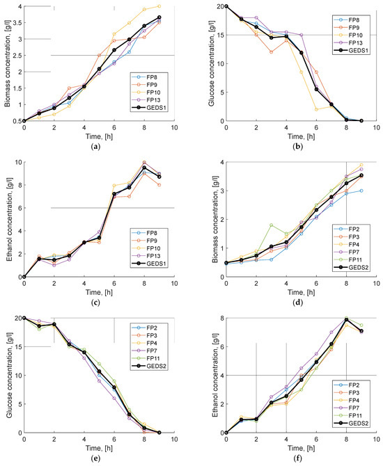
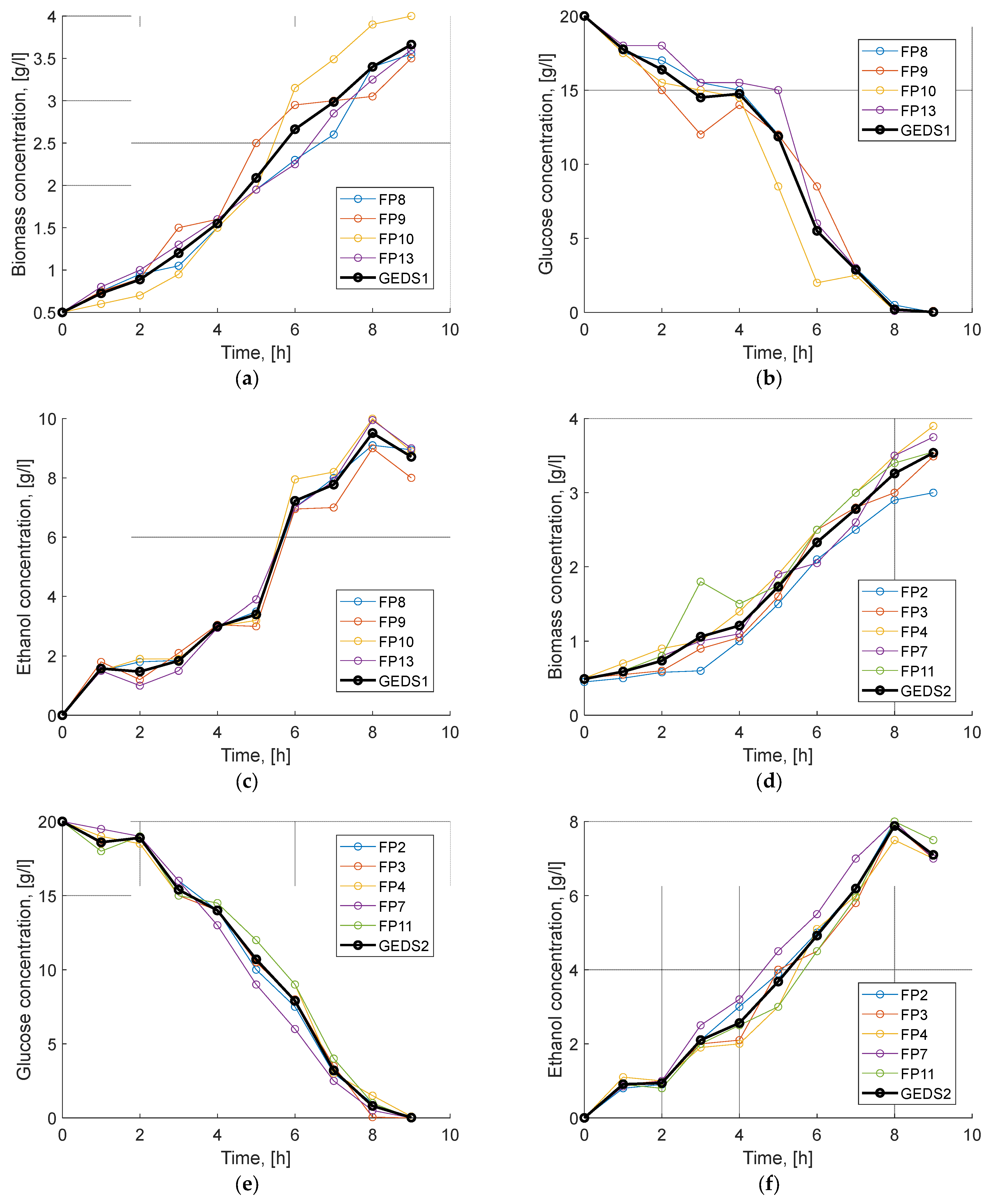
Based on the results in Table 2 and Table 3, it is concluded that FP8, FP9, FP10, and FP13 form the first core cluster (Cluster 1), representing the highest-performance K. marxianus fermentation processes. Analogically, FP2, FP3, FP4, FP7, and FP11 form the second core cluster (Cluster 2), representing the moderate-to-good performance group. The time profiles for all datasets within these two clusters are shown in Figure 7. The experimental data for each of the two clusters is arithmetically averaged. The resulting average profiles per cluster (average biomass, glucose, and ethanol concentrations), termed General Experimental Dataset 1 (GEDS1) and General Experimental Dataset 2 (GEDS2), are subsequently presented.
Figure 7.
Dataset clustering, based on PCA and ICrA—variables’ dynamics of fermentation processes in the cluster and averaged cluster data (GEDS1 or GEDS2): (a) biomass concentrations, Cluster 1; (b) glucose concentrations, Cluster 1; (c) ethanol concentrations, Cluster 1; (d) biomass concentrations, Cluster 2; (e) glucose concentrations, Cluster 2; (f) ethanol concentrations, Cluster 2.
The construction of GEDS1 and GEDS2 via arithmetic averaging across strains represents the collective phenotypic response of each cluster. Time-scale alignment was ensured as all processes were sampled at identical intervals (10 points) under synchronized batch conditions. Although averaging reduces individual strain-specific variability, it acts as a ‘metabolic consensus’ filter that highlights the fundamental kinetic behaviors shared by the group, providing a more robust foundation for model parameter identification compared to any single-strain dataset.
The first set (GEDS1) is used for model parameter identification, and the second set (GEDS2) is reserved for subsequent model verification.
5. Results and Discussion
For the structure and parameter identification, four distinct kinetic equations describing the specific glucose consumption rate () are tested. These kinetic equations, denoted as Structure 1 through Structure 4, are defined as follows:
- Structure 1. Monod kinetics [38] with specific glucose consumption rate:
- Structure 2. Noncompetitive inhibition formulated by Galvanauskas et al. [39]:
- Structure 3. Competitive inhibition by substrate and product, described by Cockshott and Bogle [40]:
- Structure 4. Competitive inhibition by product, Alba and Calvo [41]:
To facilitate model comparison, the values of the RSS (Equation (1)) and the Akaike Information Criterion (AIC) are calculated. The AIC score is used for statistical model selection, penalizing model complexity:
where N is the number of experimental data points, and K is the number of model parameters.
To comprehensively investigate the fermentation process behavior, Structures 1 to 4 are tested for all 17 datasets. The optimal model parameters are identified using the EA approach. The obtained model parameter estimates and the corresponding model errors for all strains are provided in Appendix B. For brevity, Table 4 represents only the results for the dataset classified into Cluster 1 and Cluster 2 (based on PCA and ICrA).
Table 4.
Structure and parameter identification for the representative fermentation processes of both clusters (Cluster 1 in blue; Cluster 2 in red).
The simulation results for each of the 17 K. marxianus strains reveal differences in kinetic behavior and model fit, underscoring the critical necessity of a strain-specific modelling framework. The outcomes can be summarized as follows:
- Structure 2 (Galvanauskas): This structure provided the superior fit for strains 7, 9, 11, 12, and 17. The Galvanauskas model [39] with non-linear non-competitive inhibition effectively captured the delayed onset of ethanol inhibition. The resulting fit indicated a sharp transition between growth and ethanol production, which is consistent with experimental dynamics. Notably, Strain 9 exhibited the highest substrate uptake and ethanol yield, but also the highest sensitivity to ethanol inhibition. Strains 11 and 12 showed moderate inhibition dynamics, with the data aligning well with a slower ethanol accumulation rate and sustained substrate consumption. Strain 17 demonstrated the fastest glucose depletion but exhibited premature stagnation of ethanol formation, which was accurately matched by its specific, high inhibition sensitivity.
- Structure 3 (Cockshott-Bogle): This structure provided the best overall fit for strains 1–6, 8, 10, and 13–16 (a total of 13 out of 17 datasets). The Cockshott-Bogle model [40] effectively captures ethanol inhibition through a quadratic function applied to the inhibition term. Strains 1–6 demonstrated accurate reproduction of all three characteristic fermentation phases: lag, exponential growth, and stationary. An excellent fit in ethanol accumulation was specifically observed for Strain 1. Strains 2 and 3 exhibited fast substrate depletion, while Strain 4 was characterized by the longest lag phase. Strain 14 indicated the highest ethanol tolerance. Notably, Strain 16 had exceptionally high estimated parameter values, which successfully explained its rapid ethanol production and sharp biomass rise, validating its status as a kinetic outlier.
Based on the comparative analysis of the four kinetic structures across 17 datasets, Structure 3 (Cockshott-Bogle) demonstrated the most robust statistical performance. This structure yielded the lowest average AIC values across the majority (13/17) of the high-performance strains. While no single kinetic model can be considered a universal ‘best representation’ in an absolute sense for all biological variations, Structure 3 provides the most effective relative balance between model complexity and descriptive accuracy for a representative fermentation model.
In the subsequent step, the parameters for the selected optimal model (Structure 3) are identified using the dataset GEDS1, which represents the average profiles of the high-performance strains (Cluster 1). The model parameter identification is performed using the EA. The obtained optimal model parameters are listed in Table 5.
Table 5.
Parameter identification results of the developed representative cluster-based model (Structure 3).
The estimated maximum specific growth rates and kinetic constants fall within ranges commonly reported for batch ethanol fermentation of K. marxianus [3,8,29] under comparable substrate concentrations and temperature conditions. Similarly, the identified yield coefficients are strictly positive, of realistic magnitude, and consistent with the expected coupling between biomass growth, glucose uptake, and ethanol production.
The non-integer yield values are biologically acceptable, as these parameters represent lumped, macroscopic stoichiometric relationships rather than single elementary biochemical reactions. Such effective parameters are commonly used in structured and unstructured fermentation models to capture the net outcome of complex intracellular processes.
The estimated model parameters are quantitatively consistent with the average parameter values presented in Table 3. The resulting AIC value (–18.56) for the model is statistically superior to the best individual AIC value observed for the strain-specific models in Table 3 (e.g., –17.51).
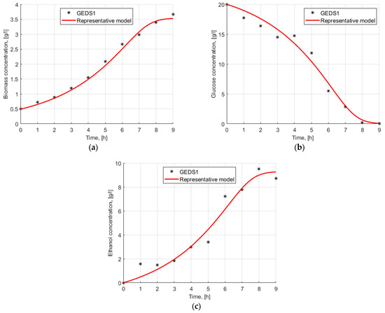
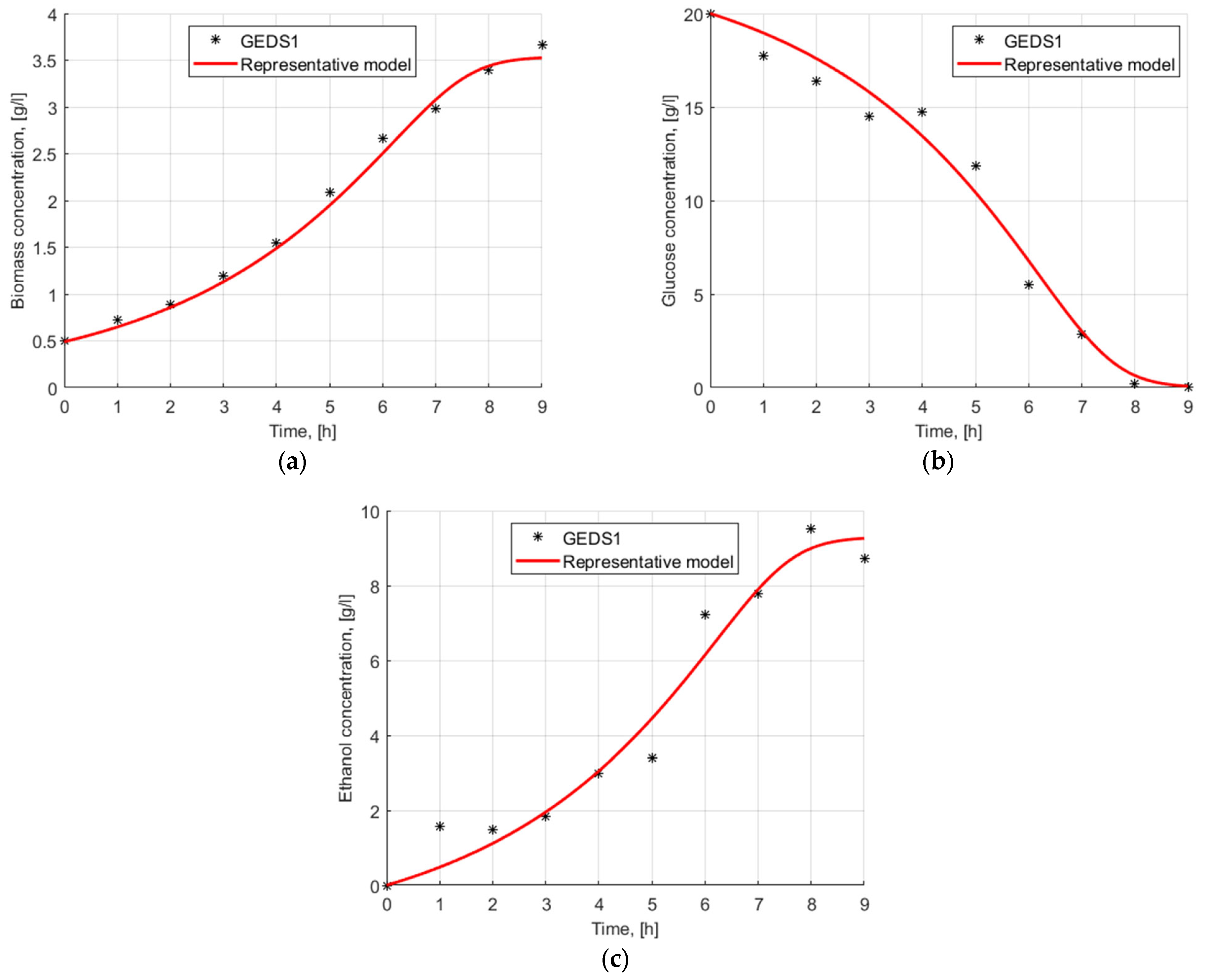
Figure 8 graphically compares the model dynamics to the GEDS1 data.
Figure 8.
Graphical comparison between first averaged general experimental dataset (GEDS1) and resulting representative cluster-based model dynamics: (a) biomass concentration; (b) glucose concentration; (c) ethanol concentration.
The presented results demonstrate an excellent fit of the model to the training dataset. The biomass dynamics exhibit strong concordance regarding the trend and magnitude approximation to the datasets. The results for the glucose concentration profiles are even more accurate, confirming the preliminary data analysis regarding the uniform kinetic pattern of glucose consumption across the microbial strains.
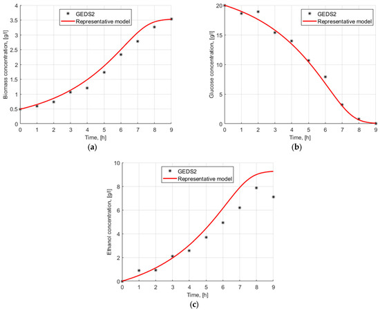
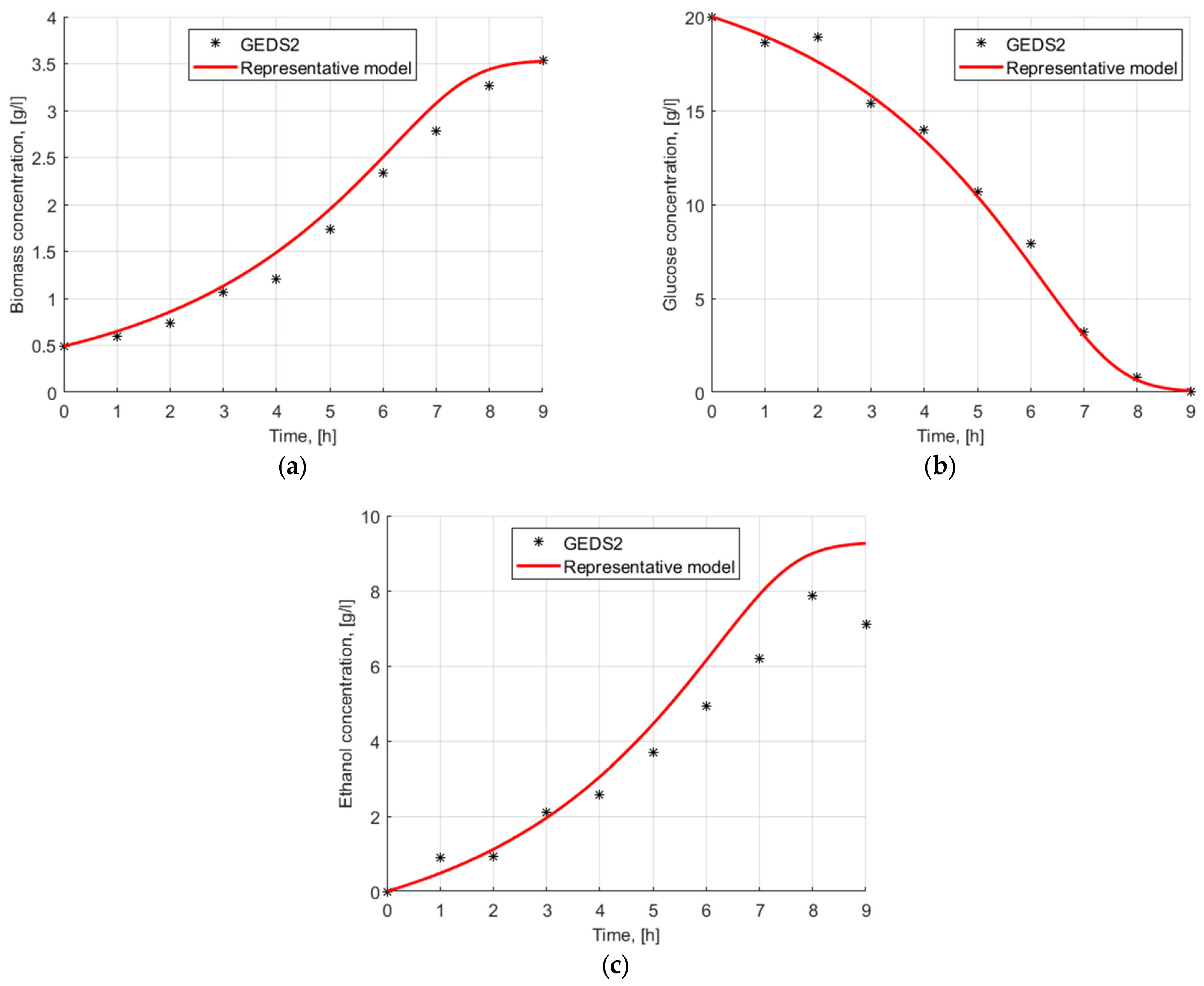
The obtained representative model (with parameters from Table 5) was subsequently verified using the independent validation dataset, GEDS2 (average profiles of Cluster 2). The model was evaluated for its ability to reproduce the average dynamics of this second, independent group of processes (GEDS2). A graphical comparison of the GEDS2 data and the model predictions is presented in Figure 9.
Figure 9.
Model verification—comparison between second averaged general experimental dataset (GEDS2) and resulting representative cluster-based model dynamics: (a) biomass concentration; (b) glucose concentration; (c) ethanol concentration.
The verification of the biomass and glucose dynamics is highly successful, with the obtained model showing very strong agreement for biomass and glucose dynamics. However, the model does not replicate ethanol dynamics with the same level of accuracy, particularly towards the final stage of the fermentation process.
The resulting verification statistics are AIC = −5.3640 and RSS = 1.76. The observed discrepancies in the verification results are primarily attributed to the error in fitting the ethanol profile. This profile was previously identified as the most sensitive and strain-specific process variable. In future research endeavors, a deeper data analysis is warranted to more accurately fit the dynamics of ethanol.
Nonetheless, the results demonstrate a high degree of accuracy for the developed representative (cluster-based) mathematical model of the K. marxianus fermentation process and confirm its verification on an independent cluster-average dataset.
The validation of the model against GEDS2 (independent dataset) yielded results that were successful in capturing the primary growth and substrate consumption trends. However, a more critical examination reveals a slight reduction in the precision of ethanol prediction for this validation group compared to the training set (GEDS1). This divergence is attributed to the inherent biological variability in secondary metabolic pathways between the ‘high-performance’ cluster (training) and the ‘moderate-performance’ cluster (validation). While the model remains a functional general tool, the lower precision in ethanol prediction for GEDS2 highlights the limitations of using a single set of generalized parameters to account for all strain-specific yield variations.
The findings of this study highlight an inherent tension in bioprocess modeling: the balance between strain-specific precision and the practical utility of a representative model. While individual kinetic parameters for each of the 17 strains would provide higher local accuracy, such an approach lacks the scalability required for industrial applications involving mixed or uncharacterized strains. Therefore, the proposed model is framed not as a universal biological law, but as a representative compromise. It identifies the consensus metabolic behavior of K. marxianus under specified conditions, serving as a robust baseline for process control while acknowledging that extreme strain-specific variations may still require local calibration.
6. Conclusions
The study presents a methodology for the processing and development of a representative cluster-based mathematical model representing a class of microorganisms (K. marxianus), encompassing 17 industrially relevant strains used for the biosynthesis of a common target product—ethanol. The proposed approach comprises the following main steps:
- Data compilation: Involves the construction of a database aggregating experimental results from all available batch fermentations associated with the production of the selected target compound.
- Initial modelling: Entails the development of a mathematical model employing the GDM approach and investigations of four different kinetic structures for the specific glucose consumption rate (Monod, Alba-Calvo, Galvanauskas, and Cockshott-Bogle kinetics).
- Clustering analysis: Requires the application of several techniques for cluster analysis of the compiled data. Two versions of PCA are utilized to identify and form primary-level clusters. These clusters are subsequently refined using ICrA, resulting in the selection of the most representative fermentations, which define the core clusters–designated Clusters 1 and 2.
- Model identification: Structure and parameter identification are conducted for all fermentation processes, including the processes in the two primary clusters. AIC and RSS criteria are employed to select the optimal model structure.
- Generalization and verification: Averaged databases are created for Cluster 1 and Cluster 2, termed GEDS1 and GEDS2. Parameter identification is performed based on the GEDS1 using the previously selected optimal model structure—Structure 3. The obtained representative model is validated against the dataset GEDS2.
As a result, a representative (cluster-based) mathematical model is developed and demonstrates strong predictive performance for the studied conditions. The model shows excellent agreement with the training cluster-average data (GEDS1) and is validated on the independent cluster-average dataset (GEDS2).
The proposed model performs most reliably for strains classified within the ‘high-performance’ cluster (Cluster 1), particularly in predicting biomass (X) and substrate (S) dynamics. For these variables, the model provides a dependable basis for process monitoring. However, caution is advised when interpreting ethanol (P) predictions for strains exhibiting ‘moderate’ or ‘anomalous’ metabolic behaviors (Clusters 2 and 3). In these cases, the observed discrepancies suggest that while the model structure is sound, local re-calibration of yield coefficients may be necessary to account for strain-specific metabolic shifts in byproduct formation.
The comparison of the newly proposed model and the model presented in [3] confirmed that the developed model is a logical evolution of existing mechanistic models. It preserves interpretability while expanding applicability and resolution within the studied class of strains and experimental conditions.
While metaheuristic algorithms are effective for navigating the non-linear and multi-modal parameter space of fermentation models, they possess inherent limitations. Specifically, these stochastic methods do not guarantee the identification of the global optimum within a finite number of iterations. In this study, the ‘stagnation’ of the fitness function and the sensitivity to initial parameter bounds were mitigated by performing multiple independent runs. However, the computational cost associated with high-dimensional searches remains a factor when scaling to more complex multi-stage kinetic structures.
In accordance with the No Free Lunch Theorem, which posits that no single metaheuristic is universally superior, the applied EA is not an absolute optimum, but is the most effective computational compromise tailored to the highly non-linear and complex kinetics of K. marxianus.
The methodology presented here enables the construction of robust, representative models that effectively capture the complex kinetic behavior of diverse microbial strains used in industrial bioprocesses, thereby supporting rational process optimization and successful scale-up endeavors. The developed model can be used to further derivation of the advanced algorithms for monitoring and control of this class of processes.
Author Contributions
Conceptualization, M.I., O.R. and V.L.; methodology, M.I., O.R. and V.L.; software, M.I., V.L., O.R., A.Z., D.K. G.R. and D.Z.; validation, M.I., O.R., A.Z. and V.L.; formal analysis, M.I., V.L., O.R., A.Z., D.K. and G.R.; investigation, M.I., V.L., O.R., A.Z., D.K. and G.R.; writing—original draft preparation, M.I., V.L., O.R., A.Z., D.K. and G.R.; writing—review and editing, M.I., O.R., V.L. and D.Z.; visualization, A.Z., D.K., G.R. and D.Z.; funding acquisition—D.Z. All authors have read and agreed to the published version of the manuscript.
Funding
This study is financed by the European Union-NextGenerationEU, through the National Recovery and Resilience Plan of the Republic of Bulgaria, project № BG-RRP-2.004-0008-C01.
Data Availability Statement
The data supporting the findings of the present work are available through the authors S.Y.; V.P.A.; R.E.; S.-C.N.O.; P.-J.B.; R.-S.F.J., upon reasonable request.
Acknowledgments
O.R. thanks the support of the Centre of Excellence in Informatics and ICT under Grant No BG16RFPR002-1.014-0018-C01, financed by the Research, Innovation and Digitalization for Smart Transformation Programme 2021–2027 and co-financed by the European Union.
Conflicts of Interest
The authors declare no conflicts of interest.
Abbreviations
The following abbreviations are used in this manuscript:
| GDM | General Dynamic Model |
| PCA | Principal Component Analysis |
| ICrA | InterCriteria Analysis |
| AIC | Akaike Information Criterion |
| RSS | Residual Sum of Squares |
| GP | Gas Phase |
| LP | Liquid Phase |
| FP | Fermentation Process |
Appendix A
Appendix A.1
Input index matrices for ICrA are index matrix of data for biomass concentrations (IM1); index matrix of data for glucose concentrations (IM2); and index matrix of data for ethanol concentrations (IM3). The index matrices consist of all experimental data (10 points) for all 17 fermentation processes, for each process variable.
| IM1 = | 1 | 2 | 3 | 4 | 5 | 6 | 7 | 8 | 9 | 10 |
| FP1 | ||||||||||
| FP2 | ||||||||||
| … | biomass concentrations | |||||||||
| FP16 | ||||||||||
| FP17 | ||||||||||
| IM2 = | 1 | 2 | 3 | 4 | 5 | 6 | 7 | 8 | 9 | 10 |
| FP1 | ||||||||||
| FP2 | ||||||||||
| … | glucose concentrations | |||||||||
| FP16 | ||||||||||
| FP17 | ||||||||||
| IM3 = | 1 | 2 | 3 | 4 | 5 | 6 | 7 | 8 | 9 | 10 |
| FP1 | ||||||||||
| FP2 | ||||||||||
| … | ethanol concentrations | |||||||||
| FP16 | ||||||||||
| FP17 | ||||||||||
Appendix A.2
Output results from ICrA gives the agreement/correlations between each two fermentation processes, based on the corresponding process variable.
IMs of the results based on biomass data
| FP1 | FP2 | FP3 | FP4 | FP5 | FP6 | FP7 | FP8 | FP9 | FP10 | FP11 | FP12 | FP13 | FP14 | FP15 | FP16 | FP17 | |
| FP1 | 1.00 | 0.98 | 0.98 | 0.98 | 0.98 | 0.98 | 0.98 | 0.98 | 0.98 | 0.98 | 0.93 | 0.98 | 0.98 | 0.98 | 0.98 | 0.89 | 0.91 |
| FP2 | 0.98 | 1.00 | 1.00 | 1.00 | 1.00 | 1.00 | 1.00 | 1.00 | 1.00 | 1.00 | 0.96 | 1.00 | 1.00 | 1.00 | 1.00 | 0.91 | 0.93 |
| FP3 | 0.98 | 1.00 | 1.00 | 1.00 | 1.00 | 1.00 | 1.00 | 1.00 | 1.00 | 1.00 | 0.96 | 1.00 | 1.00 | 1.00 | 1.00 | 0.91 | 0.93 |
| FP4 | 0.98 | 1.00 | 1.00 | 1.00 | 1.00 | 1.00 | 1.00 | 1.00 | 1.00 | 1.00 | 0.96 | 1.00 | 1.00 | 1.00 | 1.00 | 0.91 | 0.93 |
| FP5 | 0.98 | 1.00 | 1.00 | 1.00 | 1.00 | 1.00 | 1.00 | 1.00 | 1.00 | 1.00 | 0.96 | 1.00 | 1.00 | 1.00 | 1.00 | 0.91 | 0.93 |
| FP6 | 0.98 | 1.00 | 1.00 | 1.00 | 1.00 | 1.00 | 1.00 | 1.00 | 1.00 | 1.00 | 0.96 | 1.00 | 1.00 | 1.00 | 1.00 | 0.91 | 0.93 |
| FP7 | 0.98 | 1.00 | 1.00 | 1.00 | 1.00 | 1.00 | 1.00 | 1.00 | 1.00 | 1.00 | 0.96 | 1.00 | 1.00 | 1.00 | 1.00 | 0.91 | 0.93 |
| FP8 | 0.98 | 1.00 | 1.00 | 1.00 | 1.00 | 1.00 | 1.00 | 1.00 | 1.00 | 1.00 | 0.96 | 1.00 | 1.00 | 1.00 | 1.00 | 0.91 | 0.93 |
| FP9 | 0.98 | 1.00 | 1.00 | 1.00 | 1.00 | 1.00 | 1.00 | 1.00 | 1.00 | 1.00 | 0.96 | 1.00 | 1.00 | 1.00 | 1.00 | 0.91 | 0.93 |
| FP10 | 0.98 | 1.00 | 1.00 | 1.00 | 1.00 | 1.00 | 1.00 | 1.00 | 1.00 | 1.00 | 0.96 | 1.00 | 1.00 | 1.00 | 1.00 | 0.91 | 0.93 |
| FP11 | 0.93 | 0.96 | 0.96 | 0.96 | 0.96 | 0.96 | 0.96 | 0.96 | 0.96 | 0.96 | 1.00 | 0.96 | 0.96 | 0.96 | 0.96 | 0.91 | 0.98 |
| FP12 | 0.98 | 1.00 | 1.00 | 1.00 | 1.00 | 1.00 | 1.00 | 1.00 | 1.00 | 1.00 | 0.96 | 1.00 | 1.00 | 1.00 | 1.00 | 0.91 | 0.93 |
| FP13 | 0.98 | 1.00 | 1.00 | 1.00 | 1.00 | 1.00 | 1.00 | 1.00 | 1.00 | 1.00 | 0.96 | 1.00 | 1.00 | 1.00 | 1.00 | 0.91 | 0.93 |
| FP14 | 0.98 | 1.00 | 1.00 | 1.00 | 1.00 | 1.00 | 1.00 | 1.00 | 1.00 | 1.00 | 0.96 | 1.00 | 1.00 | 1.00 | 1.00 | 0.91 | 0.93 |
| FP15 | 0.98 | 1.00 | 1.00 | 1.00 | 1.00 | 1.00 | 1.00 | 1.00 | 1.00 | 1.00 | 0.96 | 1.00 | 1.00 | 1.00 | 1.00 | 0.91 | 0.93 |
| FP16 | 0.89 | 0.91 | 0.91 | 0.91 | 0.91 | 0.91 | 0.91 | 0.91 | 0.91 | 0.91 | 0.91 | 0.91 | 0.91 | 0.91 | 0.91 | 1.00 | 0.93 |
| FP17 | 0.91 | 0.93 | 0.93 | 0.93 | 0.93 | 0.93 | 0.93 | 0.93 | 0.93 | 0.93 | 0.98 | 0.93 | 0.93 | 0.93 | 0.93 | 0.93 | 1.00 |
| FP1 | FP2 | FP3 | FP4 | FP5 | FP6 | FP7 | FP8 | FP9 | FP10 | FP11 | FP12 | FP13 | FP14 | FP15 | FP16 | FP17 | |
| FP1 | 0.00 | 0.00 | 0.00 | 0.00 | 0.00 | 0.00 | 0.00 | 0.00 | 0.00 | 0.00 | 0.04 | 0.00 | 0.00 | 0.00 | 0.00 | 0.09 | 0.07 |
| FP2 | 0.00 | 0.00 | 0.00 | 0.00 | 0.00 | 0.00 | 0.00 | 0.00 | 0.00 | 0.00 | 0.04 | 0.00 | 0.00 | 0.00 | 0.00 | 0.09 | 0.07 |
| FP3 | 0.00 | 0.00 | 0.00 | 0.00 | 0.00 | 0.00 | 0.00 | 0.00 | 0.00 | 0.00 | 0.04 | 0.00 | 0.00 | 0.00 | 0.00 | 0.09 | 0.07 |
| FP4 | 0.00 | 0.00 | 0.00 | 0.00 | 0.00 | 0.00 | 0.00 | 0.00 | 0.00 | 0.00 | 0.04 | 0.00 | 0.00 | 0.00 | 0.00 | 0.09 | 0.07 |
| FP5 | 0.00 | 0.00 | 0.00 | 0.00 | 0.00 | 0.00 | 0.00 | 0.00 | 0.00 | 0.00 | 0.04 | 0.00 | 0.00 | 0.00 | 0.00 | 0.09 | 0.07 |
| FP6 | 0.00 | 0.00 | 0.00 | 0.00 | 0.00 | 0.00 | 0.00 | 0.00 | 0.00 | 0.00 | 0.04 | 0.00 | 0.00 | 0.00 | 0.00 | 0.09 | 0.07 |
| FP7 | 0.00 | 0.00 | 0.00 | 0.00 | 0.00 | 0.00 | 0.00 | 0.00 | 0.00 | 0.00 | 0.04 | 0.00 | 0.00 | 0.00 | 0.00 | 0.09 | 0.07 |
| FP8 | 0.00 | 0.00 | 0.00 | 0.00 | 0.00 | 0.00 | 0.00 | 0.00 | 0.00 | 0.00 | 0.04 | 0.00 | 0.00 | 0.00 | 0.00 | 0.09 | 0.07 |
| FP9 | 0.00 | 0.00 | 0.00 | 0.00 | 0.00 | 0.00 | 0.00 | 0.00 | 0.00 | 0.00 | 0.04 | 0.00 | 0.00 | 0.00 | 0.00 | 0.09 | 0.07 |
| FP10 | 0.00 | 0.00 | 0.00 | 0.00 | 0.00 | 0.00 | 0.00 | 0.00 | 0.00 | 0.00 | 0.04 | 0.00 | 0.00 | 0.00 | 0.00 | 0.09 | 0.07 |
| FP11 | 0.04 | 0.04 | 0.04 | 0.04 | 0.04 | 0.04 | 0.04 | 0.04 | 0.04 | 0.04 | 0.00 | 0.04 | 0.04 | 0.04 | 0.04 | 0.09 | 0.02 |
| FP12 | 0.00 | 0.00 | 0.00 | 0.00 | 0.00 | 0.00 | 0.00 | 0.00 | 0.00 | 0.00 | 0.04 | 0.00 | 0.00 | 0.00 | 0.00 | 0.09 | 0.07 |
| FP13 | 0.00 | 0.00 | 0.00 | 0.00 | 0.00 | 0.00 | 0.00 | 0.00 | 0.00 | 0.00 | 0.04 | 0.00 | 0.00 | 0.00 | 0.00 | 0.09 | 0.07 |
| FP14 | 0.00 | 0.00 | 0.00 | 0.00 | 0.00 | 0.00 | 0.00 | 0.00 | 0.00 | 0.00 | 0.04 | 0.00 | 0.00 | 0.00 | 0.00 | 0.09 | 0.07 |
| FP15 | 0.00 | 0.00 | 0.00 | 0.00 | 0.00 | 0.00 | 0.00 | 0.00 | 0.00 | 0.00 | 0.04 | 0.00 | 0.00 | 0.00 | 0.00 | 0.09 | 0.07 |
| FP16 | 0.09 | 0.09 | 0.09 | 0.09 | 0.09 | 0.09 | 0.09 | 0.09 | 0.09 | 0.09 | 0.09 | 0.09 | 0.09 | 0.09 | 0.09 | 0.00 | 0.07 |
| FP17 | 0.07 | 0.07 | 0.07 | 0.07 | 0.07 | 0.07 | 0.07 | 0.07 | 0.07 | 0.07 | 0.02 | 0.07 | 0.07 | 0.07 | 0.07 | 0.07 | 0.00 |
IMs of the results based on glucose data
| FP1 | FP2 | FP3 | FP4 | FP5 | FP6 | FP7 | FP8 | FP9 | FP10 | FP11 | FP12 | FP13 | FP14 | FP15 | FP16 | FP17 | |
| FP1 | 1.00 | 0.98 | 0.98 | 1.00 | 0.98 | 0.96 | 1.00 | 1.00 | 0.93 | 0.98 | 0.98 | 1.00 | 0.96 | 0.93 | 0.98 | 0.96 | 1.00 |
| FP2 | 0.98 | 1.00 | 1.00 | 0.98 | 0.98 | 0.93 | 0.98 | 0.98 | 0.91 | 0.96 | 1.00 | 0.98 | 0.96 | 0.91 | 0.96 | 0.93 | 0.98 |
| FP3 | 0.98 | 1.00 | 1.00 | 0.98 | 0.98 | 0.93 | 0.98 | 0.98 | 0.91 | 0.96 | 1.00 | 0.98 | 0.96 | 0.91 | 0.96 | 0.93 | 0.98 |
| FP4 | 1.00 | 0.98 | 0.98 | 1.00 | 0.98 | 0.96 | 1.00 | 1.00 | 0.93 | 0.98 | 0.98 | 1.00 | 0.96 | 0.93 | 0.98 | 0.96 | 1.00 |
| FP5 | 0.98 | 0.98 | 0.98 | 0.98 | 1.00 | 0.93 | 0.98 | 0.98 | 0.91 | 0.96 | 0.98 | 0.98 | 0.98 | 0.91 | 0.96 | 0.93 | 0.98 |
| FP6 | 0.96 | 0.93 | 0.93 | 0.96 | 0.93 | 1.00 | 0.96 | 0.96 | 0.93 | 0.93 | 0.93 | 0.96 | 0.93 | 0.98 | 0.96 | 0.93 | 0.96 |
| FP7 | 1.00 | 0.98 | 0.98 | 1.00 | 0.98 | 0.96 | 1.00 | 1.00 | 0.93 | 0.98 | 0.98 | 1.00 | 0.96 | 0.93 | 0.98 | 0.96 | 1.00 |
| FP8 | 1.00 | 0.98 | 0.98 | 1.00 | 0.98 | 0.96 | 1.00 | 1.00 | 0.93 | 0.98 | 0.98 | 1.00 | 0.96 | 0.93 | 0.98 | 0.96 | 1.00 |
| FP9 | 0.93 | 0.91 | 0.91 | 0.93 | 0.91 | 0.93 | 0.93 | 0.93 | 1.00 | 0.91 | 0.91 | 0.93 | 0.91 | 0.93 | 0.93 | 0.91 | 0.93 |
| FP10 | 0.98 | 0.96 | 0.96 | 0.98 | 0.96 | 0.93 | 0.98 | 0.98 | 0.91 | 1.00 | 0.96 | 0.98 | 0.93 | 0.91 | 0.96 | 0.96 | 0.98 |
| FP11 | 0.98 | 1.00 | 1.00 | 0.98 | 0.98 | 0.93 | 0.98 | 0.98 | 0.91 | 0.96 | 1.00 | 0.98 | 0.96 | 0.91 | 0.96 | 0.93 | 0.98 |
| FP12 | 1.00 | 0.98 | 0.98 | 1.00 | 0.98 | 0.96 | 1.00 | 1.00 | 0.93 | 0.98 | 0.98 | 1.00 | 0.96 | 0.93 | 0.98 | 0.96 | 1.00 |
| FP13 | 0.96 | 0.96 | 0.96 | 0.96 | 0.98 | 0.93 | 0.96 | 0.96 | 0.91 | 0.93 | 0.96 | 0.96 | 1.00 | 0.91 | 0.98 | 0.96 | 0.96 |
| FP14 | 0.93 | 0.91 | 0.91 | 0.93 | 0.91 | 0.98 | 0.93 | 0.93 | 0.93 | 0.91 | 0.91 | 0.93 | 0.91 | 1.00 | 0.93 | 0.91 | 0.93 |
| FP15 | 0.98 | 0.96 | 0.96 | 0.98 | 0.96 | 0.96 | 0.98 | 0.98 | 0.93 | 0.96 | 0.96 | 0.98 | 0.98 | 0.93 | 1.00 | 0.98 | 0.98 |
| FP16 | 0.96 | 0.93 | 0.93 | 0.96 | 0.93 | 0.93 | 0.96 | 0.96 | 0.91 | 0.96 | 0.93 | 0.96 | 0.96 | 0.91 | 0.98 | 1.00 | 0.96 |
| FP17 | 1.00 | 0.98 | 0.98 | 1.00 | 0.98 | 0.96 | 1.00 | 1.00 | 0.93 | 0.98 | 0.98 | 1.00 | 0.96 | 0.93 | 0.98 | 0.96 | 1.00 |
| FP1 | FP2 | FP3 | FP4 | FP5 | FP6 | FP7 | FP8 | FP9 | FP10 | FP11 | FP12 | FP13 | FP14 | FP15 | FP16 | FP17 | |
| FP1 | 0.00 | 0.02 | 0.02 | 0.00 | 0.00 | 0.02 | 0.00 | 0.00 | 0.02 | 0.02 | 0.02 | 0.00 | 0.00 | 0.04 | 0.00 | 0.00 | 0.00 |
| FP2 | 0.02 | 0.00 | 0.00 | 0.02 | 0.00 | 0.04 | 0.02 | 0.02 | 0.04 | 0.04 | 0.00 | 0.02 | 0.00 | 0.07 | 0.02 | 0.02 | 0.02 |
| FP3 | 0.02 | 0.00 | 0.00 | 0.02 | 0.00 | 0.04 | 0.02 | 0.02 | 0.04 | 0.04 | 0.00 | 0.02 | 0.00 | 0.07 | 0.02 | 0.02 | 0.02 |
| FP4 | 0.00 | 0.02 | 0.02 | 0.00 | 0.00 | 0.02 | 0.00 | 0.00 | 0.02 | 0.02 | 0.02 | 0.00 | 0.00 | 0.04 | 0.00 | 0.00 | 0.00 |
| FP5 | 0.00 | 0.00 | 0.00 | 0.00 | 0.00 | 0.02 | 0.00 | 0.00 | 0.02 | 0.02 | 0.00 | 0.00 | 0.00 | 0.04 | 0.00 | 0.00 | 0.00 |
| FP6 | 0.02 | 0.04 | 0.04 | 0.02 | 0.02 | 0.00 | 0.02 | 0.02 | 0.00 | 0.04 | 0.04 | 0.02 | 0.00 | 0.02 | 0.00 | 0.00 | 0.02 |
| FP7 | 0.00 | 0.02 | 0.02 | 0.00 | 0.00 | 0.02 | 0.00 | 0.00 | 0.02 | 0.02 | 0.02 | 0.00 | 0.00 | 0.04 | 0.00 | 0.00 | 0.00 |
| FP8 | 0.00 | 0.02 | 0.02 | 0.00 | 0.00 | 0.02 | 0.00 | 0.00 | 0.02 | 0.02 | 0.02 | 0.00 | 0.00 | 0.04 | 0.00 | 0.00 | 0.00 |
| FP9 | 0.02 | 0.04 | 0.04 | 0.02 | 0.02 | 0.00 | 0.02 | 0.02 | 0.00 | 0.04 | 0.04 | 0.02 | 0.00 | 0.00 | 0.00 | 0.00 | 0.02 |
| FP10 | 0.02 | 0.04 | 0.04 | 0.02 | 0.02 | 0.04 | 0.02 | 0.02 | 0.04 | 0.00 | 0.04 | 0.02 | 0.02 | 0.07 | 0.02 | 0.00 | 0.02 |
| FP11 | 0.02 | 0.00 | 0.00 | 0.02 | 0.00 | 0.04 | 0.02 | 0.02 | 0.04 | 0.04 | 0.00 | 0.02 | 0.00 | 0.07 | 0.02 | 0.02 | 0.02 |
| FP12 | 0.00 | 0.02 | 0.02 | 0.00 | 0.00 | 0.02 | 0.00 | 0.00 | 0.02 | 0.02 | 0.02 | 0.00 | 0.00 | 0.04 | 0.00 | 0.00 | 0.00 |
| FP13 | 0.00 | 0.00 | 0.00 | 0.00 | 0.00 | 0.00 | 0.00 | 0.00 | 0.00 | 0.02 | 0.00 | 0.00 | 0.00 | 0.02 | 0.00 | 0.00 | 0.00 |
| FP14 | 0.04 | 0.07 | 0.07 | 0.04 | 0.04 | 0.02 | 0.04 | 0.04 | 0.00 | 0.07 | 0.07 | 0.04 | 0.02 | 0.00 | 0.02 | 0.02 | 0.04 |
| FP15 | 0.00 | 0.02 | 0.02 | 0.00 | 0.00 | 0.00 | 0.00 | 0.00 | 0.00 | 0.02 | 0.02 | 0.00 | 0.00 | 0.02 | 0.00 | 0.00 | 0.00 |
| FP16 | 0.00 | 0.02 | 0.02 | 0.00 | 0.00 | 0.00 | 0.00 | 0.00 | 0.00 | 0.00 | 0.02 | 0.00 | 0.00 | 0.02 | 0.00 | 0.00 | 0.00 |
| FP17 | 0.00 | 0.02 | 0.02 | 0.00 | 0.00 | 0.02 | 0.00 | 0.00 | 0.02 | 0.02 | 0.02 | 0.00 | 0.00 | 0.04 | 0.00 | 0.00 | 0.00 |
IMs of the results based on ethanol data
| FP1 | FP2 | FP3 | FP4 | FP5 | FP6 | FP7 | FP8 | FP9 | FP10 | FP11 | FP12 | FP13 | FP14 | FP15 | FP16 | FP17 | |
| FP1 | 1.00 | 0.96 | 0.96 | 0.98 | 0.89 | 0.89 | 0.96 | 0.96 | 0.96 | 0.93 | 0.98 | 0.93 | 0.96 | 0.91 | 0.96 | 0.89 | 0.93 |
| FP2 | 0.96 | 1.00 | 1.00 | 0.98 | 0.93 | 0.93 | 0.98 | 1.00 | 0.96 | 0.98 | 0.98 | 0.98 | 0.96 | 0.96 | 0.96 | 0.89 | 0.98 |
| FP3 | 0.96 | 1.00 | 1.00 | 0.98 | 0.93 | 0.93 | 0.98 | 1.00 | 0.96 | 0.98 | 0.98 | 0.98 | 0.96 | 0.96 | 0.96 | 0.89 | 0.98 |
| FP4 | 0.98 | 0.98 | 0.98 | 1.00 | 0.91 | 0.91 | 0.96 | 0.98 | 0.98 | 0.96 | 1.00 | 0.96 | 0.98 | 0.93 | 0.98 | 0.87 | 0.96 |
| FP5 | 0.89 | 0.93 | 0.93 | 0.91 | 1.00 | 0.96 | 0.91 | 0.93 | 0.89 | 0.93 | 0.91 | 0.91 | 0.91 | 0.93 | 0.93 | 0.82 | 0.96 |
| FP6 | 0.89 | 0.93 | 0.93 | 0.91 | 0.96 | 1.00 | 0.91 | 0.93 | 0.91 | 0.93 | 0.91 | 0.96 | 0.89 | 0.98 | 0.93 | 0.82 | 0.96 |
| FP7 | 0.96 | 0.98 | 0.98 | 0.96 | 0.91 | 0.91 | 1.00 | 0.98 | 0.93 | 0.96 | 0.96 | 0.96 | 0.93 | 0.93 | 0.93 | 0.89 | 0.96 |
| FP8 | 0.96 | 1.00 | 1.00 | 0.98 | 0.93 | 0.93 | 0.98 | 1.00 | 0.96 | 0.98 | 0.98 | 0.98 | 0.96 | 0.96 | 0.96 | 0.89 | 0.98 |
| FP9 | 0.96 | 0.96 | 0.96 | 0.98 | 0.89 | 0.91 | 0.93 | 0.96 | 1.00 | 0.93 | 0.98 | 0.96 | 0.96 | 0.93 | 0.96 | 0.84 | 0.93 |
| FP10 | 0.93 | 0.98 | 0.98 | 0.96 | 0.93 | 0.93 | 0.96 | 0.98 | 0.93 | 1.00 | 0.96 | 0.96 | 0.93 | 0.96 | 0.93 | 0.87 | 0.96 |
| FP11 | 0.98 | 0.98 | 0.98 | 1.00 | 0.91 | 0.91 | 0.96 | 0.98 | 0.98 | 0.96 | 1.00 | 0.96 | 0.98 | 0.93 | 0.98 | 0.87 | 0.96 |
| FP12 | 0.93 | 0.98 | 0.98 | 0.96 | 0.91 | 0.96 | 0.96 | 0.98 | 0.96 | 0.96 | 0.96 | 1.00 | 0.93 | 0.98 | 0.93 | 0.87 | 0.96 |
| FP13 | 0.96 | 0.96 | 0.96 | 0.98 | 0.91 | 0.89 | 0.93 | 0.96 | 0.96 | 0.93 | 0.98 | 0.93 | 1.00 | 0.91 | 0.96 | 0.84 | 0.93 |
| FP14 | 0.91 | 0.96 | 0.96 | 0.93 | 0.93 | 0.98 | 0.93 | 0.96 | 0.93 | 0.96 | 0.93 | 0.98 | 0.91 | 1.00 | 0.91 | 0.84 | 0.93 |
| FP15 | 0.96 | 0.96 | 0.96 | 0.98 | 0.93 | 0.93 | 0.93 | 0.96 | 0.96 | 0.93 | 0.98 | 0.93 | 0.96 | 0.91 | 1.00 | 0.84 | 0.98 |
| FP16 | 0.89 | 0.89 | 0.89 | 0.87 | 0.82 | 0.82 | 0.89 | 0.89 | 0.84 | 0.87 | 0.87 | 0.87 | 0.84 | 0.84 | 0.84 | 1.00 | 0.87 |
| FP17 | 0.93 | 0.98 | 0.98 | 0.96 | 0.96 | 0.96 | 0.96 | 0.98 | 0.93 | 0.96 | 0.96 | 0.96 | 0.93 | 0.93 | 0.98 | 0.87 | 1.00 |
| FP1 | FP2 | FP3 | FP4 | FP5 | FP6 | FP7 | FP8 | FP9 | FP10 | FP11 | FP12 | FP13 | FP14 | FP15 | FP16 | FP17 | |
| FP1 | 0.00 | 0.04 | 0.04 | 0.02 | 0.11 | 0.09 | 0.02 | 0.04 | 0.04 | 0.04 | 0.02 | 0.04 | 0.02 | 0.07 | 0.04 | 0.09 | 0.07 |
| FP2 | 0.04 | 0.00 | 0.00 | 0.02 | 0.07 | 0.04 | 0.00 | 0.00 | 0.04 | 0.00 | 0.02 | 0.00 | 0.02 | 0.02 | 0.04 | 0.09 | 0.02 |
| FP3 | 0.04 | 0.00 | 0.00 | 0.02 | 0.07 | 0.04 | 0.00 | 0.00 | 0.04 | 0.00 | 0.02 | 0.00 | 0.02 | 0.02 | 0.04 | 0.09 | 0.02 |
| FP4 | 0.02 | 0.02 | 0.02 | 0.00 | 0.09 | 0.07 | 0.02 | 0.02 | 0.02 | 0.02 | 0.00 | 0.02 | 0.00 | 0.04 | 0.02 | 0.11 | 0.04 |
| FP5 | 0.11 | 0.07 | 0.07 | 0.09 | 0.00 | 0.02 | 0.07 | 0.07 | 0.11 | 0.04 | 0.09 | 0.07 | 0.07 | 0.04 | 0.07 | 0.16 | 0.04 |
| FP6 | 0.09 | 0.04 | 0.04 | 0.07 | 0.02 | 0.00 | 0.04 | 0.04 | 0.07 | 0.02 | 0.07 | 0.04 | 0.07 | 0.02 | 0.04 | 0.13 | 0.02 |
| FP7 | 0.02 | 0.00 | 0.00 | 0.02 | 0.07 | 0.04 | 0.00 | 0.00 | 0.04 | 0.00 | 0.02 | 0.00 | 0.02 | 0.02 | 0.04 | 0.07 | 0.02 |
| FP8 | 0.04 | 0.00 | 0.00 | 0.02 | 0.07 | 0.04 | 0.00 | 0.00 | 0.04 | 0.00 | 0.02 | 0.00 | 0.02 | 0.02 | 0.04 | 0.09 | 0.02 |
| FP9 | 0.04 | 0.04 | 0.04 | 0.02 | 0.11 | 0.07 | 0.04 | 0.04 | 0.00 | 0.04 | 0.02 | 0.02 | 0.02 | 0.04 | 0.04 | 0.13 | 0.07 |
| FP10 | 0.04 | 0.00 | 0.00 | 0.02 | 0.04 | 0.02 | 0.00 | 0.00 | 0.04 | 0.00 | 0.02 | 0.00 | 0.02 | 0.00 | 0.04 | 0.09 | 0.02 |
| FP11 | 0.02 | 0.02 | 0.02 | 0.00 | 0.09 | 0.07 | 0.02 | 0.02 | 0.02 | 0.02 | 0.00 | 0.02 | 0.00 | 0.04 | 0.02 | 0.11 | 0.04 |
| FP12 | 0.04 | 0.00 | 0.00 | 0.02 | 0.07 | 0.04 | 0.00 | 0.00 | 0.02 | 0.00 | 0.02 | 0.00 | 0.02 | 0.02 | 0.04 | 0.09 | 0.02 |
| FP13 | 0.02 | 0.02 | 0.02 | 0.00 | 0.07 | 0.07 | 0.02 | 0.02 | 0.02 | 0.02 | 0.00 | 0.02 | 0.00 | 0.04 | 0.02 | 0.11 | 0.04 |
| FP14 | 0.07 | 0.02 | 0.02 | 0.04 | 0.04 | 0.02 | 0.02 | 0.02 | 0.04 | 0.00 | 0.04 | 0.02 | 0.04 | 0.00 | 0.07 | 0.11 | 0.04 |
| FP15 | 0.04 | 0.04 | 0.04 | 0.02 | 0.07 | 0.04 | 0.04 | 0.04 | 0.04 | 0.04 | 0.02 | 0.04 | 0.02 | 0.07 | 0.00 | 0.13 | 0.02 |
| FP16 | 0.09 | 0.09 | 0.09 | 0.11 | 0.16 | 0.13 | 0.07 | 0.09 | 0.13 | 0.09 | 0.11 | 0.09 | 0.11 | 0.11 | 0.13 | 0.00 | 0.11 |
| FP17 | 0.07 | 0.02 | 0.02 | 0.04 | 0.04 | 0.02 | 0.02 | 0.02 | 0.07 | 0.02 | 0.04 | 0.02 | 0.04 | 0.04 | 0.02 | 0.11 | 0.00 |
The ICrA clusters are defined based on the obtained values of the degree of agreement and the degree of disagreement between each pair of FPs. After several iterations of ranking, the fermentations are clustered into three groups listed in Table 2.
Appendix B
Table A1.
Model parameter estimates for each kinetic structure, based on 17 different experimental datasets.
References
- Lane, M.M.; Morrissey, J.P. Kluyveromyces marxianus: A yeast emerging from its sister’s shadow. Fungal Biol. Rev. 2010, 24, 17–26. [Google Scholar] [CrossRef] [Scilit]
- Margaritis, A.; Bajpai, P. Direct Fermentation of d-Xylose to Ethanol by Kluyveromyces marxianus Strains. Appl. Environ. Microbiol. 1982, 44, 1039–1041. [Google Scholar] [CrossRef] [Scilit] [PubMed]
- Salazar, Y.; Valle, P.A.; Rodríguez, E.; Soto-Cruz, N.O.; Páez-Lerma, J.B.; Reyes-Sánchez, F.J. Mechanistic modelling of biomass growth, glucose consumption and ethanol production by Kluyveromyces marxianus in batch fermentation. Entropy 2023, 25, 497. [Google Scholar] [CrossRef] [Scilit] [PubMed]
- Zafar, S.; Owais, M. Ethanol production from crude whey by Kluyveromyces marxianus. Biochem. Eng. J. 2006, 27, 295–298. [Google Scholar] [CrossRef] [Scilit]
- Mo, W.; Wang, M.; Zhan, R.; Yu, Y.; He, Y.; Lu, H. Kluyveromyces marxianus developing ethanol tolerance during adaptive evolution with significant improvements of multiple pathways. Biotechnol. Biofuels 2019, 12, 63. [Google Scholar] [CrossRef] [Scilit]
- Ariyanti, D.; Hadiyanto, H. Ethanol production from whey by Kluyveromyces marxianus in batch fermentation system: Kinetics parameters estimation. Bull. Chem. React. Eng. Catal. 2013, 7, 179–184. [Google Scholar] [CrossRef]
- Hadiyanto, H.; Ariyanti, D.; Aini, A.P.; Pinundi, D.S. Batch and fed-batch fermentation system on ethanol production from whey using Kluyveromyces marxianus. Int. J. Renew. Energy Dev. 2013, 2, 127. [Google Scholar] [CrossRef] [Scilit]
- Ariyanti, D.; Aini, A.P.; Pinundi, D.S. Optimization of ethanol production from whey through fed-batch fermentation using Kluyveromyces marxianus. Energy Procedia 2014, 47, 108–112. [Google Scholar] [CrossRef] [Scilit]
- Bastin, G.; Dochain, D. On-Line Estimation and Adaptive Control of Bioreactors; Elsevier: Amsterdam, The Netherlands, 1990. [Google Scholar]
- Lyubenova, V.; Zoteva, D.; Ignatova, M.; Kristeva, D.; Roeva, O. A System Designed for Modelling, Monitoring, and Control of Fermentation Processes, Powered by Metaheuristic Algorithms. Processes 2025, 13, 1632. [Google Scholar] [CrossRef] [Scilit]
- Tomar, V.; Bansal, M.; Singh, P. Metaheuristic algorithms for optimization: A brief review. Eng. Proc. 2024, 59, 238. [Google Scholar]
- Peres, F.; Castelli, M. Combinatorial optimization problems and metaheuristics: Review, challenges, design, and development. Appl. Sci. 2021, 11, 6449. [Google Scholar] [CrossRef] [Scilit]
- Vincent, A.M.; Jidesh, P. An improved hyperparameter optimization framework for AutoML systems using evolutionary algorithms. Sci. Rep. 2023, 13, 4737. [Google Scholar] [CrossRef] [Scilit] [PubMed]
- Tilman, A.R.; Vasconcelos, V.V.; Akçay, E.; Plotkin, J.B. The evolution of forecasting for decision-making in dynamic environments. Collect. Intell. 2023, 2, 26339137231221726. [Google Scholar] [CrossRef] [Scilit]
- de Araújo Costa, A.P.; Choren, R.; de Moura Pereira, D.A.; Terra, A.V.; de Araújo Costa, I.P.; de Souza Rocha Junior, C.; Santos, M.D.; Gomes, C.F.S.; Moreira, M.Â.L. Integrating Multicriteria Decision Making and Principal Component Analysis: A Systematic Literature Review. Cogent Eng. 2024, 11, 2374944. [Google Scholar] [CrossRef] [Scilit]
- Mafata, M.; Brand, J.; Kidd, M.; Medvedovici, A.; Buica, A. Exploration of Data Fusion Strategies Using Principal Component Analysis and Multiple Factor Analysis. Beverages 2022, 8, 66. [Google Scholar] [CrossRef] [Scilit]
- Maugeri, A.; Barchitta, M.; Favara, G.; La Mastra, C.; La Rosa, M.C.; Magnano San Lio, R.; Agodi, A. The Application of Clustering on Principal Components for Nutritional Epidemiology: A Workflow to Derive Dietary Patterns. Nutrients 2023, 15, 195. [Google Scholar] [CrossRef] [Scilit]
- Singh, M.; Pant, M.; Kong, L.; Alijani, Z.; Snasel, V. A PCA-Based Fuzzy Tensor Evaluation Model for Multiple-Criteria Group Decision Making. Appl. Soft Comput. 2023, 132, 109753. [Google Scholar] [CrossRef] [Scilit]
- Dong, W.; Woźniak, M.; Wu, J.; Li, W.; Bai, Z. Denoising Aggregation of Graph Neural Networks by Using Principal Component Analysis. IEEE Trans. Ind. Inform. 2023, 19, 2385–2394. [Google Scholar] [CrossRef] [Scilit]
- Atanassov, K.; Mavrov, D.; Atanassova, V. Intercriteria Decision Making: A New Approach for Multicriteria Decision Making, Based on Index Matrices and Intuitionistic Fuzzy Sets. Issues IFSs GNs 2014, 11, 1–8. [Google Scholar]
- Atanassov, K. Intuitionistic Fuzzy Sets. VII ITKR Session, Sofia, 20–23 June 1983. Center for Science and Technology, Library of the Bulgaria, Academy of Sciences: Sofia, Bulgaria. Repr. Int. J. Bioautom. 2016, 20, S1–S6. [Google Scholar]
- Atanassov, K. Review and New Results on Intuitionistic Fuzzy Sets. Int. J. Bioautom. 2016, 20, S7–S16. [Google Scholar]
- Atanassov, K. Index Matrices: Towards an Augmented Matrix Calculus; Springer: Berlin/Heidelberg, Germany, 2014; Volume 573, Available online: https://link.springer.com/book/10.1007/978-3-319-10945-9 (accessed on 21 January 2026).
- Chorukova, E.; Marinov, P.; Umlenski, I. Survey on Theory and Applications of InterCriteria Analysis Approach. In Research in Computer Science in the Bulgarian Academy of Sciences; Study Computer Intelligence; Atanassov, K.T., Ed.; Springer: Cham, Switzerland, 2021; Volume 934. [Google Scholar] [CrossRef] [Scilit]
- Todinova, S.; Mavrov, D.; Krumova, S.; Marinov, P.; Atanassova, V.; Atanassov, K.; Taneva, S.G. Blood Plasma Thermograms Dataset Analysis by Means of InterCriteria and Correlation Analyses for the Case of Colorectal Cancer. Int. J. Bioautom. 2016, 20, 115–124. [Google Scholar]
- Shiskova, I.; Stratiev, D.; Tavlieva, M.; Nedelchev, A.; Dinkov, R.; Kolev, I.; van den Berg, F.; Ribagin, S.; Sotirov, S.; Nikolova, R.; et al. Application of Intercriteria and Regression Analyses and Artificial Neural Network to Investigate the Relation of Crude Oil Assay Data to Oil Compatibility. Processes 2024, 12, 780. [Google Scholar] [CrossRef] [Scilit]
- Jekova, I.; Vassilev, P.; Stoyanov, T.; Pencheva, T. InterCriteria Analysis: Application for ECG Data Analysis. Mathematics 2021, 9, 854. [Google Scholar] [CrossRef] [Scilit]
- Petrov, M.; Ilkova, T. Intercriteria decision analysis for choice of growth rate models of batch cultivation by strain Kluyveromyces marxianus var. lactis MC 5. J. Int. Sci. Publ. Mater. Methods Technol. 2016, 10, 468–486. [Google Scholar]
- Petrov, M.; Ilkova, T.; Vanags, J. Modelling of a Batch Whey Cultivation of Kluyveromyces marxianus var. lactis MC 5 with Investigation of Mass Transfer Processes in the Bioreactor. Int. J. Bioautom. 2015, 19, S81–S92. [Google Scholar]
- Tinôco, D.; Silveira, W.B. Kinetic model of ethanol inhibition for Kluyveromyces marxianus CCT 7735 (UFV-3) based on the modified Monod model by Ghose & Tyagi. Biologia 2021, 76, 3511–3519. [Google Scholar] [CrossRef] [Scilit]
- Sansonetti, S.; Hobley, T.J.; Calabrò, V.; Villadsen, J.; Sin, G. A biochemically structured model for ethanol fermentation by Kluyveromyces marxianus: A batch fermentation and kinetic study. Bioresour. Technol. 2011, 102, 7513–7520. [Google Scholar] [CrossRef] [Scilit]
- Lyubenova, V.; Kostov, G.; Denkova-Kostova, R. Model-based monitoring of biotechnological processes—A review. Processes 2021, 9, 908. [Google Scholar] [CrossRef] [Scilit]
- Lyubenova, V.; Ignatova, M.; Zoteva, D.; Roeva, O. Model-Based Adaptive Control of Bioreactors—A Brief Review. Mathematics 2024, 12, 2205. [Google Scholar] [CrossRef] [Scilit]
- Zlatkova, A.; Lyubenova, V.; Dudin, S.; Ignatova, M. Marker for switching of multiple models describing E. coli cultivation. Comptes Rendus L’académie Bulg. Sci. 2017, 70, 263–272. [Google Scholar]
- Corne, D.; Lones, M.A. Evolutionary Algorithms. In Handbook of Heuristics; Martí, R., Pardalos, P.M., Resende, M.G., Eds.; Springer: Cham, Switzerland, 2025. [Google Scholar] [CrossRef] [Scilit]
- Páez-Lerma, J.B.; Arias-García, A.; Rutiaga-Quiñones, O.M.; Barrio, E.; Soto-Cruz, N.O. Yeasts isolated from the alcoholic 559 fermentation of Agave duranguensis during mezcal production. Food Biotechnol. 2013, 27, 342–356. [Google Scholar] [CrossRef] [Scilit]
- Paredes-Ortíz, A.; Olvera-Martínez, T.; Páez-Lerma, J.; Rojas-Contreras, J.; Moreno-Jiménez, M.; Aguilar, C.; Soto-Cruz, N. 562 Isoamyl acetate production during continuous culture of Pichia fermentans. Rev. Mex. Ing. Química 2022, 563, Bio2654. [Google Scholar] [CrossRef] [Scilit]
- Monod, J. The growth of bacterial cultures. Annu. Rev. Microbiol. 1949, 3, 371–394. [Google Scholar] [CrossRef] [Scilit]
- Galvanauskas, V.; Simutis, R.; Volk, N.; Lübert, A. Model based design of a biochemical cultivation process. Bioprocess. Eng. 1998, 18, 227–234. [Google Scholar] [CrossRef] [Scilit]
- Cockshott, A.R.; Bogle, I.D.L. Modelling a recombinant E. coli fermentation producing bovine somatotropin. IFAC Proc. Vol. 1992, 2, 219–222. [Google Scholar]
- Alba, M.J.G.; Calvo, E.G. Characterization of bioreaction processes: Aerobic Escherichia coli cultures. J. Biotechnol. 2000, 84, 107–118. [Google Scholar] [CrossRef] [Scilit]
- Shahapure, K.R.; Nicholas, C. Cluster Quality Analysis Using Silhouette Score. In Proceedings of the 2020 IEEE 7th International Conference on Data Science and Advanced Analytics (DSAA), Sydney, NSW, Australia, 6–9 October 2020; pp. 747–748. [Google Scholar] [CrossRef] [Scilit]
- Shutaywi, M.; Kachouie, N.N. Silhouette Analysis for Performance Evaluation in Machine Learning with Applications to Clustering. Entropy 2021, 23, 759. [Google Scholar] [CrossRef] [Scilit]

Disclaimer/Publisher’s Note: The statements, opinions and data contained in all publications are solely those of the individual author(s) and contributor(s) and not of MDPI and/or the editor(s). MDPI and/or the editor(s) disclaim responsibility for any injury to people or property resulting from any ideas, methods, instructions or products referred to in the content. |
© 2026 by the authors. Licensee MDPI, Basel, Switzerland. This article is an open access article distributed under the terms and conditions of the Creative Commons Attribution (CC BY) license.