Article

The Health-Wealth Gradient in Labor Markets: Integrating Health, Insurance, and Social Metrics to Predict Employment Density

1
School of Engineering and Applied Science, University of Pennsylvania, Philadelphia, PA 19104, USA
2
Graduate School of Art and Science, Boston University, Boston, MA 02215, USA
3
School of Professional Studies, Columbia University, New York, NY 10027, USA
*
Author to whom correspondence should be addressed.
These authors contributed equally to this work.
Computation 2026, 14(1), 22; https://doi.org/10.3390/computation14010022
Submission received: 20 December 2025 / Revised: 3 January 2026 / Accepted: 10 January 2026 / Published: 15 January 2026

Abstract

Labor market forecasting relies heavily on economic time-series data, often overlooking the “health–wealth” gradient that links population health to workforce participation. This study develops a machine learning framework integrating non-traditional health and social metrics to predict state-level employment density. Methods: We constructed a multi-source longitudinal dataset (2014–2024) by aggregating county-level Quarterly Census of Employment and Wages (QCEW) data with County Health Rankings to the state level. Using a time-aware split to evaluate performance across the COVID-19 structural break, we compared LASSO, Random Forest, and regularized XGBoost models, employing SHAP values for interpretability. Results: The tuned, regularized XGBoost model achieved strong out-of-sample performance (Test R 2 = 0.800). A leakage-safe stacked Ridge ensemble yielded comparable performance (Test R 2 = 0.827), while preserving the interpretability of the underlying tree model used for SHAP analysis.

1. Introduction

The ability [1] to predict labor market trends functions as a core element which enables successful economic policy implementation and effective regional development planning. The development of these forecasts has followed a historical pattern based on the business cycle paradigm in which economists used econometric models including vector autoregression (VAR) and ARIMA time-series methods [2]. The established frameworks use previous unemployment rates and GDP data to generate their predictions about future employment statistics. The method relies on the belief that economic output determines labor market behavior because capital investment and output demand control the system which allows researchers to predict future performance through analysis of past economic data [3].
The current economic structure with its complex design system has made it clear that the previous method does not work effectively. Linear models succeed in detecting general market patterns which occur during times of market stability but they become less effective when dealing with the complex non-linear relationships that exist in contemporary economic systems [4,5]. The current established frameworks fail because they maintain strict structures which separate labor market analysis from the actual health of workers and their environment. Standard forecasting systems which only use monetary and production data make two incorrect assumptions about human labor because they fail to recognize that human population workability faces multiple biological and social barriers.
The current situation has become unsustainable because new research proves that national economic performance directly depends on population health. The “health–wealth” gradient demonstrates that workers need more than job availability to participate in the workforce because they must also possess the capability to accept available positions [6]. This gradient operates through bidirectional channels: economic stability enables access to health resources, while physiological and psychological well-being determines an individual’s capacity to supply labor. The health–wealth framework recognizes that chronic conditions and social instability can structurally exclude prime-age workers from the labor force entirely. Consequently, understanding labor market density requires analyzing these upstream health determinants that constrain the aggregate supply of human capital. Public health issues including obesity, substance abuse, and housing instability create major economic problems because they lead to decreased workforce involvement and reduced employee earnings [1,7]. The standard employment forecasting systems do not include these social determinants of health (SDOH) which affect population health [8]. The exclusion of particular data points happens because linear models from the past do not handle complex social information well which produces bad model results and wrong threshold value predictions that cause employees to leave the organization.
The research fills this knowledge gap through its analysis of data which extends from 2014 to 2024 and combines QCEW information with detailed County Health Rankings data. The research moves past standard linear prediction because it uses a machine learning system which detects complex patterns between variables to analyze how the “health–wealth” gradient affects state employment density. Scientists can identify intricate medical–financial relationships through this research approach which standard assessment techniques fail to detect, thus improving their ability to study labor market systems.

1.1. Research Objectives

This study aims to develop a machine learning framework that integrates non-traditional health and social metrics to predict employment density (employment per 1000 residents). Specifically, this research seeks to achieve the following:
1.
Construct a Multi-Source Longitudinal Dataset: The dataset combines economic data with public health information which includes but is not limited to obesity rates and violent crime statistics and housing problems throughout all states from 2014 to 2024.
2.
Create a forecasting pipeline based on regularized XGBoost: The research implements a time-dependent train–test split to evaluate multiple predictive models, including LASSO regression and Random Forest and regularized XGBoost with a focus on how well they perform in real-world scenarios. The Ridge ensemble model operates in stacked mode to verify if uniting different model types produces better results than the top-performing non-linear model.
3.
Examine selected feature importance for reasonableness through case study: Analyze some of the most predictive variables in Texas and New Jersey and interpret the results based on their respective characteristics. Pinpoint that the model result can help identify state-specific risk profiles, which supports strategic monitoring and sheds light on hypotheses for future causal research.

1.2. Contributions

This study contributes to the fields of labor economics, health economics, and predictive analytics in the following three distinct ways:
  • The research establishes a single-model inference which connects predictive accuracy to economic interpretations at different scales. The XGBoost model with regularization and diagnostic functions is used to analyze data at different levels of detail. The national level reveals the hierarchical structure of health and social determinants which affect employment density according to SHAP values. The state-level analysis uses mean SHAP contribution to identify essential variables which contribute most significantly to the predictions along with their directional associations. The stacked Ridge ensemble serves as a robustness checking device which demonstrates that adding more model layers does not improve predictions beyond what the regularized XGBoost model achieves.
  • Feature importance ranking together with SHAP analysis helps to establish specific positions for non-economic factors in the “Health–Wealth” relationship. The study advances from qualitative link identification to find specific numerical values which demonstrate % Excessive Drinking and % Some College outperform conventional metrics for employment density prediction.
  • By identifying specific, modifiable social determinants (such as housing instability and violent crime) as leading indicators for employment, this research offers policymakers a targeted framework. It suggests that public health and urban safety interventions work as effective indirect financial tools which create employment density growth in various labor market segments.

2. Data Sources and Preparation

2.1. Labor Market and Health Data

The empirical analysis draws on two primary data sources. Labor market outcomes are measured using the Quarterly Census of Employment and Wages (QCEW), which provides county-level employment counts by industry and quarter [9]. Population denominators are constructed from ACS-based resident population aggregates that are consistent with the geography used in the QCEW data [10].
To capture the health and social context in which local labor markets operate, we merge in county-level indicators from the County Health Rankings (CHR) [11,12]. These include measures of health behaviors (e.g., % Excessive Drinking, Teen Birth Rate), clinical care (e.g., Primary Care Physicians Rate, % Uninsured), social and economic factors (e.g., % Children in Poverty, % Children in Single-Parent Households, Social Association Rate), and the physical environment (e.g., % Severe Housing Problems, Food Environment Index, driving deaths per 100,000). The resulting dataset spans U.S. counties from 2014 to 2024, subject to data availability and suppression constraints in the underlying sources. This structure aligns with population-health frameworks that emphasize the social and economic determinants of health and labor-market outcomes [13,14,15,16,17].

2.2. Unit of Analysis and Outcome Variable

Because the ultimate goal is to understand and forecast employment at the scale at which most policy decisions are made, the analysis is conducted on a state–year panel. After aggregation and restricting to state–year observations with a non-missing outcome, the effective sample contains 539 observations over 2014–2024. The missing data are mainly due to Alaska and Michigan discontinuing their employment data reporting, with Alaska stopping in 2017 and Michigan stopping in 2022. The time-aware split yields 297 training observations (2014–2019) and 242 test observations (2020–2024). After feature screening and removal of all-NaN and constant columns, the final predictor matrix contains 32 numeric state-level features. County-level observations from QCEW and CHR are harmonized and aggregated to construct a panel covering U.S. states from 2014 to 2024. The panel is unbalanced in years where underlying employment or health data are suppressed or missing, but it includes all state–year combinations for which both employment and population can be reliably measured.
The outcome of interest is state-level employment density, defined as employment per 1000 residents in state s and year t:
employment _ per _ 1 k _ state s , t = TotalEmployment s , t ResidentPopulation s , t × 1000 .
Total employment is obtained from QCEW employment counts [9], while resident population is based on ACS-derived state–year population aggregates [10]. This normalization allows for meaningful comparisons of labor market intensity across states with different population sizes.
We select employment density rather than the traditional employment rate (employment divided by the active labor force) to better capture the full extent of the health–wealth gradient. Standard employment rates exclude “discouraged workers”, individuals who have exited the labor force entirely due to chronic health issues or disability. By using the total resident population as the denominator, the density metric accounts for the loss of human capital among those who are technically out of the labor force but might otherwise be employed if health barriers were removed. This provides a more robust measure of a region’s total productive capacity.

2.3. Construction of State-Level Predictors

All explanatory variables originate at the county level and are aggregated to the state–year level using within-state arithmetic means across counties in the same year. State-level totals used in constructing the outcome (Total Employment and Resident Population) are carried through unchanged within each state–year, as these totals are already defined at the state level in the merged panel. This aggregation procedure matches the implementation used to construct the state–year modeling dataset and is applied uniformly across the CHR indicators that enter the predictor matrix [11,12]. This aggregation strategy preserves the substantive interpretation of each measure.
The resulting dataset is a multi-source longitudinal panel in which each row corresponds to a state–year and each column corresponds to a health, social, or economic characteristic. In the modeling stage (Section 4), the sample is restricted to state–year observations with non-missing values for the outcome and the predictors used in the machine learning models.

3. Exploratory Data Analysis: Feature Validation and Spatiotemporal Dynamics

The analysis of public health economic and insurance metrics as main labor market participation predictors required us to study their normalized time-based patterns from 2014 to 2024 and their geographical spread across the United States. The research aimed to confirm that employment_per_1k_state has enough variation and relationship with this triad of variables—physiological health, economic stability, and healthcare access—to function as three separate independent predictors.

3.1. Temporal Robustness and Structural Divergence

We randomly selected a few variables, including the percentage of adults with obesity (health variable), percentage of children in poverty (economic variable), percentage of fair or poor health (health variable), and percentage of people uninsured (insurance variable), to compare their trends against our outcome variable. The longitudinal analysis across representative regions—California, Illinois, New Jersey, and Texas—confirms that our selected feature set captures both secular trends and distinct shock responses across diverse policy environments (See Figure 1a–d).

3.1.1. The 2020 Break and Health Independence

The 2020 structural break (COVID-19) functions as a testing mechanism which evaluates how different variables react to severe events. The employment data showed a distinct V-shaped pattern which included both a major decline and a quick return to previous levels (grey line). The health predictors in our model delivered distinct information which did not duplicate any existing data. The teal line showing obesity prevalence kept rising at a steady rate which separated from the economic growth pattern. The research findings validate the need to include health-related variables as these variables enable better assessment of work capacity limitations which standard economic indicators fail to measure.

3.1.2. Policy Variance and Economic Structure

Our analysis suggests that structural support systems consist of separate elements that form their individual parts. The tracking of poverty rates follows employment cycles but the % Uninsured (gold line) showed distinct patterns between different regions. The uninsured rate in California and New Jersey followed a steady downward pattern but Texas showed a unique pattern with significant fluctuations. By including insurance coverage alongside standard economic metrics, the model captures the “policy environment”—distinguishing between regions where safety nets support workforce retention versus those where structural gaps may hinder it.

3.2. Spatial Covariance and Regional Clustering

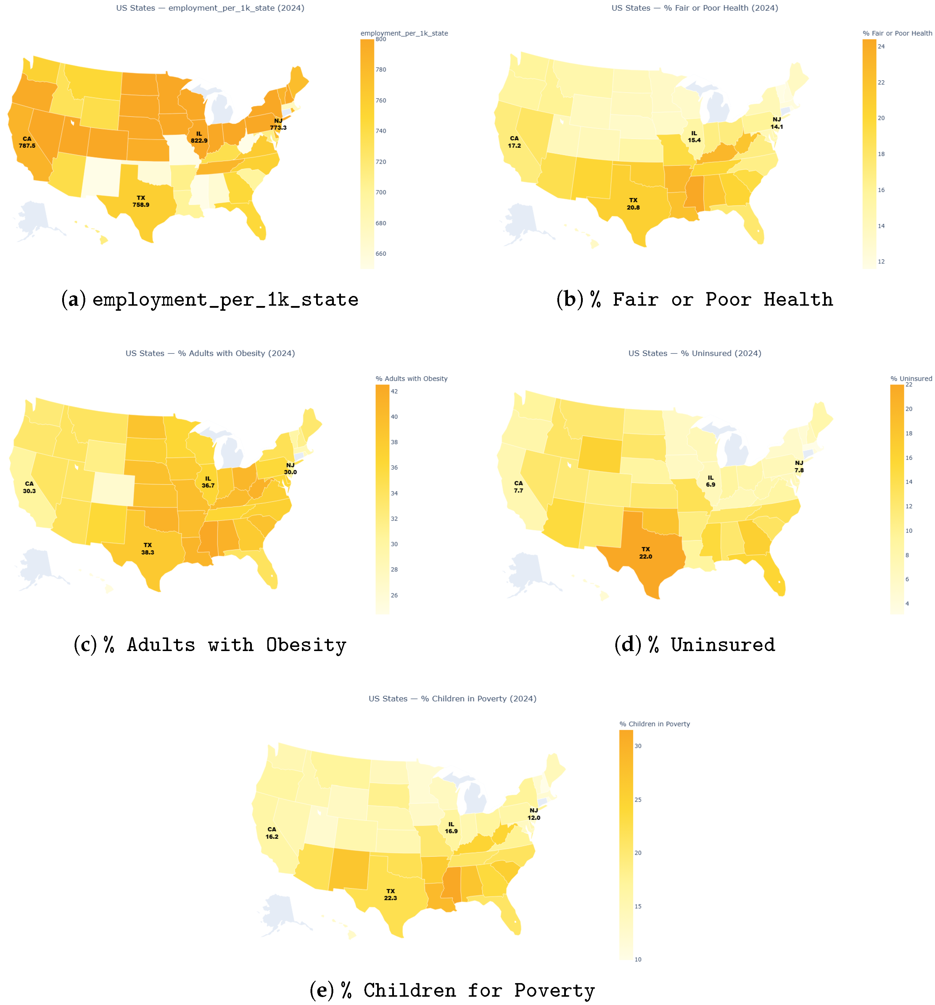
To validate the cross-sectional predictive ability of these features, we examined their spatial distribution in Fiscal Year 2024. The observed clustering confirms that labor market density directly relates to the total impact created jointly by economic factors and health issues (See Figure 2a–e).

3.2.1. The “Southern Belt” Constraints

Visual inspection reveals a strong inverse spatial correlation between employment density and structural distress such as low access to healthcare or high children poverty rate, which validates our economic and insurance predictors.

3.2.2. Structural Barriers

The “Southern Belt,” exemplified by Texas, faces two major problems. It has high poverty rates and many residents lack health insurance coverage. Conversely, New Jersey (Northeast region) and Illinois (Midwest region) show lower poverty rates and their uninsured population numbers between 6.9% and 12.0%. The gradient shows that poverty levels and insurance status serve as essential factors that enable researchers to study labor market competition between different areas.

3.2.3. Health Correlations

The health results between northern and southern regions display the same pattern as their economic separation. Texas shows high rates of poor health at 20.8% while facing economic difficulties but New Jersey shows better health results at 14.1%. The research confirms that a population with good health and insurance coverage is a prerequisite for higher employment capacity.

3.2.4. Non-Linearity in Industrial Hubs

The EDA suggests that these predictors create non-linear relationships with each other. Illinois maintains high employment numbers at 822.9 per 1 k population yet its obesity rate stands at 36.7%. The study confirms our multivariate approach since health functions as a universal negative predictor which can be impacted by strong economic drivers, and a model needs to weigh these competing factors simultaneously.

3.3. Conclusion: Justification for Feature Selection

The exploratory analysis provides empirical justification for the proposed feature set:
  • The health patterns (specifically obesity) function independently from economic market fluctuations, providing independent predictive value.
  • The percentage of uninsured population in each state captures essential policy differences between Texas and California which cannot be measured through poverty statistics alone.
  • The “Southern Belt” characteristics show a strong spatial relationship with employment density because this particular set of health, economy, and insurance metrics successfully identifies the core elements determining employment.

4. Methodology

Building on the panel described in Section 2, this section describes the modeling pipeline used to forecast state-level employment density. The procedure has three main components: (i) feature screening, data cleaning, and a time-aware train–test split; (ii) estimation of baseline and regularized prediction models; and (iii) post hoc interpretation of the selected model using SHAP values [18]. Quantitative performance results for these models are reported in Section 5. This design situates the analysis within a growing literature that uses machine learning ensembles to study unemployment and regional labor-market outcomes  [19] and complements evidence on the links between health, social conditions, and labor-market participation [13,14,20,21,22,23,24].

4.1. Feature Screening, Data Cleaning, and Time-Aware Split

Prior to statistical screening, the initial pool of predictors was selected based on established theoretical frameworks linking health and social metrics to labor supply. Following the “health–wealth” literature, we included physiological indicators (e.g., obesity, physical health days) as proxies for functional work capacity [1,6]. Social determinants such as housing stability and violent crime rates were included to capture environmental barriers to employment entry [7,13], while insurance coverage metrics were selected to reflect the safety nets that enable workforce retention [14]. This theoretical pre-selection ensures that the subsequent machine learning feature importance analysis interprets meaningful structural associations rather than spurious correlations.
To avoid mechanical leakage from variables that directly encode the outcome or its close transformations, the feature set excludes any variables that measure employment counts, hiring flows, or population denominators. In particular, variables such as Employment_Count, Employment_Count_state_sum, employment_per_1k_state, New_Hires, new_hires_per_1k, and population scalers are removed from the predictor matrix. Pure identifiers (state names, FIPS codes, year indicators) are also excluded as features.
Starting from this reduced set, only numeric columns are retained. Columns that are entirely missing or constant are dropped, resulting in a total of 32 numeric predictors. Remaining missing values are imputed using the median of each feature, which is a simple and robust approach for the modest amount of missingness present in the aggregated panel. In implementation, imputation is performed inside model pipelines (via SimpleImputer) so that imputation parameters are learned using training data only and applied to the test sample.
For linear models (LASSO and the Ridge meta-learner described below), predictors are standardized so that each feature has mean zero and unit variance in the training sample. This is implemented via a StandardScaler within a Pipeline. Tree-based models (XGBoost and Random Forest) are estimated on the unscaled feature matrix, since decision-tree splits are invariant to monotone transformations of the predictors.
Because the goal is to forecast employment density rather than merely fit historical variation, the sample is partitioned using a time-aware split. All observations with Year 2019 are assigned to the training set, and observations with Year > 2019 form the test set. This design deliberately assigns the COVID-19 period and its aftermath to the test set, so that models are evaluated on a period that is both out-of-sample and structurally different from the pre-2019 training environment.
The final analytic panel contains 539 state–year observations after aggregation and cleaning, with 297 observations in the training period (Years 2019 ) and 242 observations in the test period (Years > 2019 ). These counts reflect the effective sample used in all model comparisons after dropping rows with missing outcomes and applying feature-level median imputation within the state–year panel. To strengthen time-awareness beyond a single split, we implement walk-forward (expanding-window) evaluation by year within the training period: for each training year t, models are fit on all earlier years < t and evaluated on year t.
These walk-forward folds are used (i) for XGBoost hyperparameter tuning (train-only) and (ii) to construct out-of-fold (OOF) predictions for leakage-safe stacking. Because walk-forward OOF prediction requires prior-year information, the first two training years (2014–2015) do not receive OOF predictions and are excluded from estimation of the Ridge meta-learner.
In addition, a rolling-origin evaluation over 2018–2024 trains on all years t 1 and tests on year t, providing a year-by-year robustness check that explicitly covers the COVID shock and the post-2020 recovery. Walk-forward CV and OOF predictions are used only within the pre-2020 training period for model selection and leakage-safe stacking, whereas rolling-origin evaluation is reported as an external robustness check spanning both pre- and post-2020 years.
Model performance is summarized using the coefficient of determination R 2 , the root mean squared error (RMSE), and mean absolute error (MAE), expressed in units of employment per 1000 residents. Training metrics are reported for completeness, but the main benchmark for comparison across models is test-set performance; the corresponding statistics are presented in Section 5.

4.2. Baseline Models and Initial XGBoost Benchmark

The modeling strategy proceeds in stages. In the first stage, a set of baseline models is estimated on the state–year panel: a penalized linear model (LASSO), a lightly tuned XGBoost model, and a multi-layer perceptron (MLP). All models are fit on the same training set and evaluated on the same held-out post-2019 test set.
LASSO regression extends ordinary least squares by adding an L 1 penalty on the coefficients [25]:
min β 1 2 n i = 1 n ( y i X i β ) 2 + λ j = 1 p | β j | .
Here, λ is a tuning parameter that controls the degree of shrinkage. LASSO is implemented using LassoCV with time-aware cross-validation (walk-forward folds by year) over a grid of candidate λ values. Predictors are standardized inside the pipeline. LASSO serves as an interpretable linear benchmark and provides embedded feature selection, since the penalty can drive small coefficients exactly to zero.
The initial XGBoost and MLP models are introduced as flexible non-linear baselines. Gradient boosting, implemented via XGBRegressor [26], fits trees sequentially, with each new tree aimed at reducing the residual error of the current ensemble under a squared-error loss. The MLP is a feedforward neural network with one hidden layer and ReLU activations. As Section 5 shows, these lightly tuned models can achieve extremely tight in-sample fits but generalize poorly to the post-2019 test set, motivating a second stage focused on more conservative regularization of tree-based models and on leakage-safe ensembling.

4.3. Regularized XGBoost Specification

In the second stage, XGBoost is treated as the leading non-linear candidate model, and the focus shifts to constructing a more conservative, regularized specification designed to preserve predictive power while improving out-of-sample stability [26].
The final regularized XGBoost configuration combines several forms of regularization. Tree complexity is constrained by limiting depth and tightening split criteria: a small maximum depth, a higher minimum child weight, and a positive value of the gamma parameter require a non-trivial gain in the loss function before introducing a new split. Stochasticity is introduced through subsampling, with row subsampling and column subsampling at both the tree and level stages. This reduces correlation across trees and tends to improve generalization.
In addition, explicit L 1 and L 2 penalties are imposed on the leaf weights through the parameters reg_alpha and reg_lambda, which shrink extreme leaf values and encourage a sparser internal representation. Finally, a relatively low learning rate is combined with a moderate number of boosting rounds, so that the ensemble is built gradually rather than fitting large corrections in a small number of steps.
Hyperparameters are selected using RandomizedSearchCV on the training period only (Years 2019 ), with the selection criterion based on cross-validated RMSE. Cross-validation follows a walk-forward (expanding-window) design by year: each fold trains on all earlier training years and validates on the next year. The search evaluates 60 random configurations drawn from the ranges reported in Table 1, and the final specification is the model with the lowest walk-forward CV RMSE.
The regularized configuration substantially narrows the gap between training and test performance relative to the initial baseline XGBoost model, while maintaining a high test R 2 . For this reason, it is treated as the primary non-linear forecasting model and is the version used in the subsequent SHAP-based interpretability analysis.

4.4. Stacked Ridge Ensemble as Robustness Check

The third stage of the modeling strategy examines whether combining different model classes can yield additional predictive gains. To that end, a stacked ensemble is constructed that blends the penalized LASSO, the regularized XGBoost model, and a regularized Random Forest, echoing recent work that leverages ensembles of tree-based models to analyze labor-market outcomes [19].
The stacking procedure is designed to avoid meta-learner leakage by constructing meta-features from walk-forward out-of-fold (OOF) predictions. For each training year t, each base learner is fit using all earlier training years < t and then used to predict outcomes for year t. Because walk-forward OOF prediction requires prior-year information, the first two training years (2014–2015) do not receive OOF predictions and are excluded from estimation of the Ridge meta-learner. For test-set evaluation, each base model is re-fit on the full training period (Years 2019 ) and used to generate meta-features for Years > 2019 , which are then passed through the Ridge meta-learner.
The meta-learner estimates ensemble weights γ by solving
min γ 1 2 n i = 1 n y i Z i γ 2 + α k = 1 3 γ k 2 ,
where α is an L 2 penalty parameter selected by cross-validation on the training sample.
As discussed in Section 5, the estimated weights place most of the mass on the regularized XGBoost predictions, with only small, and in some cases negative, coefficients on the LASSO and Random Forest components. Consistent with these weights, the stacked ensemble yields test statistics that are only marginally different from those of the regularized XGBoost model on its own. The ensemble is therefore treated primarily as a robustness device that confirms that no major predictive gains are left on the table by relying on the regularized XGBoost model.

4.5. Final Model Choice and SHAP Framework

Given the evidence from the baseline comparisons, the regularization of XGBoost, and the stacked ensemble, the regularized XGBoost specification is selected as the final forecasting model for the empirical results. It delivers the best balance between out-of-sample accuracy and parsimony, and it has a structure that is amenable to post hoc interpretability tools.
To open up the fitted XGBoost model and understand which variables drive its predictions, SHAP (SHapley Additive exPlanations) values [27] are computed for all state–year observations. The tree-based SHAP implementation provides, for each observation and each feature, a decomposition of the model’s prediction into additive contributions relative to a global baseline. A positive SHAP value for a feature indicates that, holding other features fixed, the observed value of that feature pushes the prediction upward relative to the average; a negative value indicates the opposite.
Section 5.3 uses these SHAP values to construct global importance rankings and to interpret the role of key health and social determinants in shaping predicted employment density.
To extend this analysis to the regional level, we further utilize the decomposable nature of SHAP values to conduct state-specific feature importance assessments. Instead of estimating separate regression models for individual states, which would suffer from degrees-of-freedom limitations given the short time-series, we isolate and aggregate the SHAP values generated by the global model for specific state subsets. The method uses the statistical strength of the complete national database to establish local connections, which enables the model to link its state-level predictions to the specific health and policy elements which define each area.
Specifically, for the comparative case studies in Section 6, we calculate the mean absolute SHAP value for each predictor within the New Jersey and Texas sub-samples. The metric functions as an excellent indicator which shows how much each variable affects employment density throughout the specified state environment during 2014 to 2024. The framework enables users to determine which health and social determinants function as main structural barriers that affect the labor market of their state through its ranking system. The framework uses this method to convert worldwide data into specific policy recommendations which target the local needs of each state.

5. Results

5.1. Baseline Models and Evidence of Overfitting

Table 2 reports the performance of three baseline models estimated on the state–year panel: LASSO, a lightly tuned XGBoost model, and a multi-layer perceptron (MLP). The time-aware split defined in Section 4 is used throughout, with observations up to 2019 in the training set and the post-2019 period reserved for testing. Model fit is summarized using R 2 , RMSE, and MAE, with errors measured in units of employment per 1000 residents.
The LASSO model delivers a strong linear benchmark. In the training sample, it attains an R 2 of 0.875 with RMSE = 46.71 and MAE = 34.77. On the test set, its R 2 is 0.675 with RMSE = 72.65 and MAE = 53.00. This drop is expected when moving from in-sample to out-of-sample evaluation, but the test performance remains relatively strong given the model’s linear form.
By contrast, the high-capacity non-linear baselines exhibit clear signs of overfitting. The baseline XGBoost specification achieves an almost perfect in-sample fit ( R 2 = 0.99996, RMSE = 0.79, MAE = 0.63), yet its test R 2 falls to 0.569 and its RMSE increases sharply to 83.64. The MLP behaves similarly: it attains a training R 2 of 0.970 (RMSE = 22.89; MAE = 16.77), but its test R 2 drops to 0.228 with RMSE = 111.93 and MAE = 89.70. These patterns indicate that, when left only lightly constrained, flexible non-linear models can fit idiosyncrasies in the pre-2020 period that do not generalize to the pandemic and post-pandemic years.

5.2. Regularized Tree Models, Leakage-Safe Stacking, and Robustness Checks

Table 3 summarizes the performance of the regularized models used in the final forecasting pipeline: LASSO, a tuned regularized XGBoost specification, a regularized Random Forest, and a stacked ensemble that combines them.
The tuned regularized XGBoost configuration described in Section 4 emerges as the strongest individual model. It achieves an in-sample training R 2 of 0.9997 with RMSE = 2.28 and MAE = 1.07. More importantly, its post-2019 test performance improves substantially relative to the baseline XGBoost model, with  R 2 = 0.800, RMSE = 56.96, and MAE = 40.10. This pattern is consistent with the idea that non-linear interactions between health and social determinants contain predictive content, but only once the model is appropriately constrained and tuned using time-aware validation.
To provide a more conservative estimate of pre-2020 forecasting accuracy (and to reduce reliance on in-sample training metrics), the code also reports walk-forward out-of-fold (OOF) performance for the tuned XGBoost model within the training period. Under this evaluation, tuned XGBoost achieves OOF R 2 = 0.899 with RMSE = 42.27 and MAE = 24.56 (Table 4), substantially less optimistic than the in-sample training fit and therefore more credible as an estimate of forecast performance in a time-series setting.
The stacked ensemble is constructed using LASSO, tuned XGBoost, and the regularized Random Forest as base learners, with a Ridge meta-learner trained only on walk-forward OOF predictions to prevent leakage. On the test set, the ensemble attains R 2 = 0.827 with RMSE = 53.00 and MAE = 38.68, representing a modest improvement over tuned XGBoost. The estimated Ridge weights place most of the mass on XGBoost (approximately 0.93), with smaller adjustments from LASSO (approximately 0.20) and Random Forest (approximately 0.08 ), indicating that the ensemble behaves largely as a slightly rescaled version of tuned XGBoost.
Finally, a rolling-origin evaluation provides a year-by-year robustness check. As presented in Table 5, the tuned XGBoost model maintains strong performance even when forecasts for each year are generated using a model trained strictly on prior years. For example, the model achieves an R 2 of 0.815 in 2020 and 0.790 in 2024. These results support the claim that the model’s performance is stable across time and is not an artifact of a single specific train/test split.

5.3. SHAP-Based Interpretation of the XGBoost Model

To interpret the fitted regularized XGBoost model, SHAP (SHapley Additive exPlanations) values [27] are computed for all state–year observations. The tree-based SHAP implementation enables users to view how each observation and feature affects model predictions through baseline-adjusted additive contributions. The SHAP values become positive when a feature leads to a prediction that exceeds the average value while all other features stay unchanged. The prediction value decreases when a feature displays negative SHAP values while all other features keep their existing values.
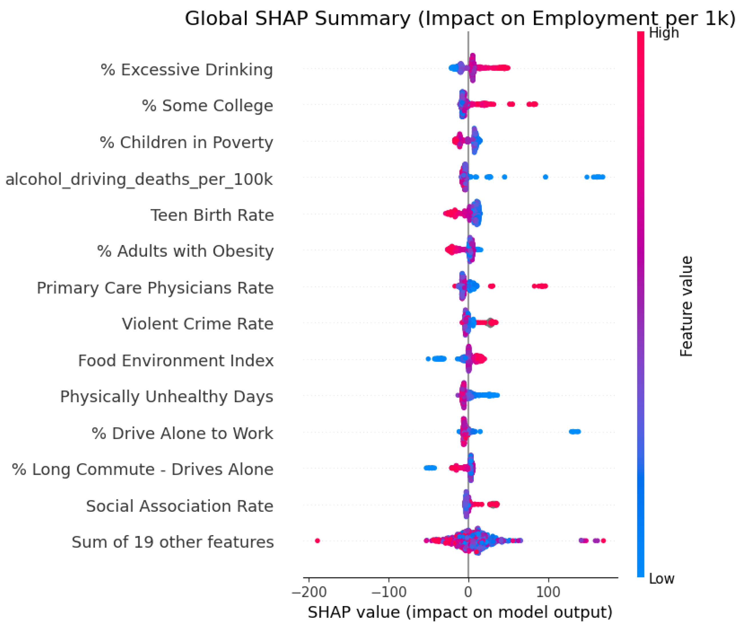
The SHAP summary plot Figure A1 demonstrates that socioeconomic status together with health environment serve as the main elements which affect employment density. % Excessive Drinking and % Some College emerge among the strongest positive contributors. This is interpreted as predictive association that may proxy for urbanization and population composition, which correlate with higher employment density. The positive college education signal shows that human capital development serves as the main statistical indicator that indicates healthy labor market conditions.
The structural disadvantage creates an effective negative warning system which functions as a powerful negative indicator. % Children in Poverty and Teen Birth Rate stand as the top two negative indicators that show the highest levels of concern. The analysis shows that states with high child poverty rates and teen birth numbers (red points) tend to appear on the left side of the zero line, which indicates that these states will have lower employment density. % Adults with Obesity shows the same pattern as before because they function as a persistent negative indicator which proves that population-level physical health deterioration leads to decreased labor market participation.
The research demonstrates that infrastructure components together with their entry points function as predictive factors which indicate what will happen in the future. The Primary Care Physicians Rate and Food Environment Index both display positive associations, where higher access to clinical care and healthy food correlates with higher predicted employment. The Violent Crime Rate variable also likely functions as a metropolitan/urbanization proxy in the state-level panel, reflecting col-linearity with density and economic activity rather than a direct beneficial effect. The combined results from these rankings show that the XGBoost model uses both socioeconomic status and healthcare accessibility data to predict which states will have high or low employment density.

Illustrated Interaction and Non-Linear Effects

The necessity of using a non-linear tree model over a linear framework is evidenced by two key findings in our results.
The performance difference between the linear baseline and the final model shows the extent to which non-linear effects impact the system. The LASSO model, which assumes purely additive relationships, capped at a test R 2 of 0.676. By enabling non-linear decision boundaries, the regularized XGBoost model improved this to 0.800. The 12.4-point increase indicates that employment density results from more than the combination of health and economic factors because health problems such as obesity create economic challenges which lead to tipping points.
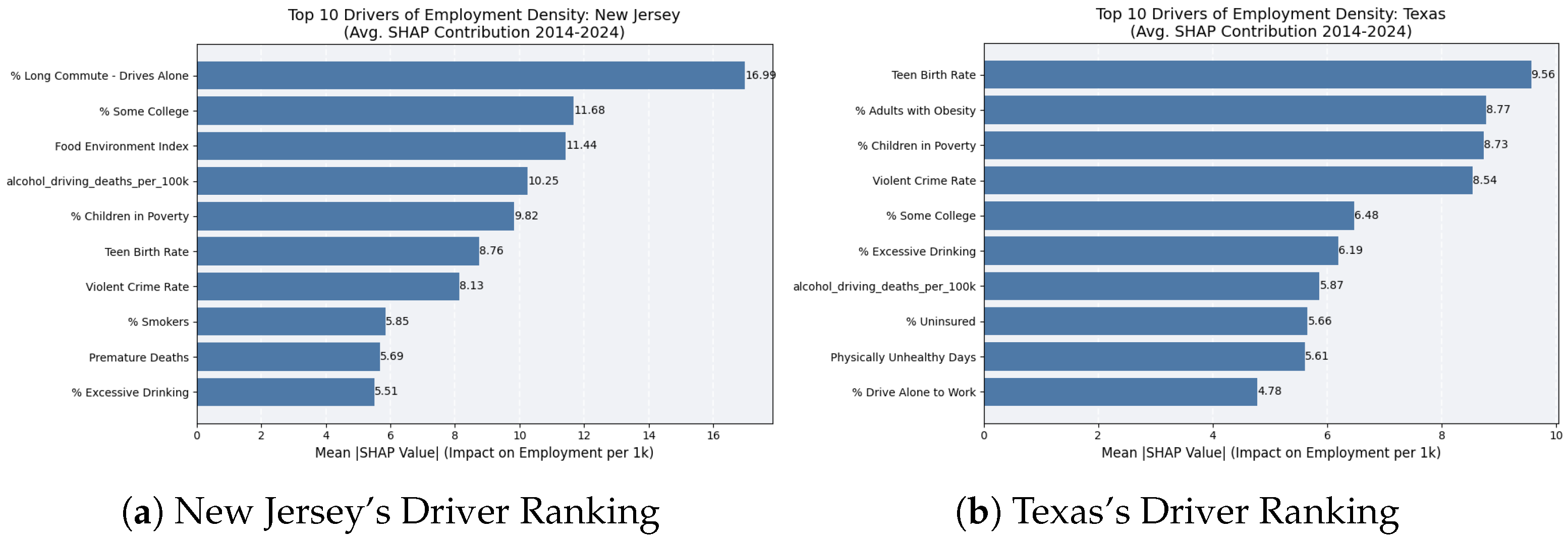
The model shows specific interaction effects which demonstrate how each variable affects prediction results when certain regional conditions exist. As detailed later in Section 6 and Figure 3, “Long Commute” emerges as the dominant driver in New Jersey, likely acting as a proxy for infrastructure connectivity. The Texas infrastructure variable gives way to social vulnerability metrics which include “Teen Birth Rate”. The economic value of transportation infrastructure depends on the existing social protection system which exists in the region.

6. Case Study—Comparative Feature Importance

To analyze regional heterogeneity in labor market predictions, we examined the SHAP values extracted from the global regularized XGBoost model specifically for the New Jersey and Texas sub-samples. The model predicts employment density by using local signals which combine state observations from 2014 to 2024 through mean absolute SHAP value aggregation. The method prevents statistical problems which occur when running separate regression models on limited state-based data while enabling detailed analysis of how different variables affect the predictions.
The research between New Jersey and Texas revealed their predictive methods operate differently because New Jersey bases its employment density forecasts on infrastructure and human capital data, yet Texas depends on social determinants of health and structural vulnerability indicators for its predictions.

6.1. State Deep Dive: New Jersey

The New Jersey predictive profile (see Figure 3a) shows that infrastructure and built-environment factors control the outcome because the state functions as a densely populated transportation route through the Northeast megalopolis. The most prominent predictor for New Jersey is Long Commute-Drives Alone, with a mean absolute SHAP contribution of 16.99. In a state like New Jersey, this variable likely captures spatial structure and job-housing geography, including access to large cross-state labor markets and commuting corridors, rather than a direct mechanism. The model therefore uses commuting intensity as a predictive marker of employment concentration and regional connectivity, not as evidence that longer commutes causally increase employment density.
The secondary indicators support the main emphasis, which centers on organizational structure and workforce abilities. % Some College (11.68) and the Food Environment Index (11.44) appear as the next most important predictors. The model shows how New Jersey employment status emerges through its indicators which use educational levels and local resource availability. The health variables Alcohol Driving Deaths and Premature Deaths in New Jersey appear at lower levels of the hierarchy, but they are still among the top 10 drivers, which indicates that health factors play a fairly important role in the state. Fundamental health issues remain influential in explaining the state’s employment density variations, alongside educational facilities and public transportation systems.

6.2. State Deep Dive: Texas

The Texas predictive framework (see Figure 3b) bases its analysis on social health determinants together with measures which show how much society disadvantages certain groups. The three most effective predictive indicators consist of Teen Birth Rate at 9.56 followed by % Adults with Obesity at 8.77 and % Children in Poverty at 8.73. The model depends on Teen Birth Rate and Child in Poverty indicators which show how the population will develop its economic potential and prepare its workforce for the future. The employment density patterns in Texas require social vulnerability and population health status variables to understand them better than the infrastructure-focused approach of New Jersey.
The structural vulnerability story becomes more visible because % Uninsured (5.66) functions as an independent risk factor which generates its own warning indicator together with Physically Unhealthy Days (5.61). The model depends on insurance status to make predictions which becomes important for Texas because the XGBoost algorithm uses insurance coverage gaps to identify labor markets with unstable conditions and high levels of informal work. The Violent Crime Rate (8.54) stands as a top indicator in this model which probably serves as an urbanization indicator to differentiate between urban economic hubs of Houston and Dallas and their rural counterparts. The variable does not directly affect economic performance but instead helps identify between urban and rural areas. The specific variables in this cluster show that Texas prediction models depend most on the “health–wealth gradient” which uses basic public health and access outcomes to determine labor market intensity.

6.3. Comparative Synthesis: Structural vs. Individual Determinants

The two states show how the global model modifies its predictive system to work in various geographical locations. The model of New Jersey uses structural data to predict its economic development because it analyzes how people commute and their educational background to determine employment density which matches a fully developed economy that depends on public transportation. The predictive signal for Texas bases its prediction on social factors because the model uses teen birth rates, obesity levels, and poverty rates to identify different labor market results.
The comparison shows that analysts can obtain important data through the combination of health and social metrics with economic information. The research demonstrates that social determinants of health function as distinct predictors which affect different states through their role as fundamental factors in some areas and their function as main indicators of economic performance in other areas.

7. Discussion

The empirical analysis in this paper demonstrates that an XGBoost gradient boosting model with regularization which uses multiple health and social factors produces accurate state employment density predictions that maintain their performance when facing disruptions such as the COVID-19 pandemic aftermath. The SHAP values in this model provide prediction explanations. They demonstrate that poverty among children and unstable housing conditions reduce the intensity of employment but educational success and helpful surroundings produce opposite effects. The case study on New Jersey and Texas confirms this finding because these states show how different factors influence health outcomes between the Northeast and South regions. The research findings provide a method to predict economic performance and create policies and combined treatment approaches. The following section presents applications, including their restrictions together with possible future developments.

7.1. Applicability to Economic Forecasting and Scenario Planning

The method produces its highest accuracy during future simulations because it improves macroeconomic models which lack understanding of non-economic elements. The time-aware validation split, which reserves the volatile post-2019 period (COVID-19 and recovery years) for the test set and keeps it out of model training, demonstrates that the forecasting pipeline can generalize to structurally different conditions shaped by health and social constraints. State economic councils or national bureaus should implement this system through real-time systems which would update health–social stream data for generating new projections. The SHAP rankings help users create hypothetical situations which show how family support programs for child poverty reduction are potentially associated with generating additional jobs in the workforce. States with high burden rates can consider maintaining their economic stability through risk management systems which focus on controlling excessive drinking and obesity. Organizations may shift their funding toward constructing enduring residential buildings because this construction will likely generate more financial benefits. The stacked ensemble system provides protection through model combination, which enables the system to process how poverty levels interact with access to care services and allows it to combine growth indicators with central bank data.

7.2. Policy Implications for Integrated Health-Economic Interventions

Our findings suggest that health–social performance indicators would benefit from integrating across different systems to develop better protection systems for workers. The main obstacles for participation stem from basic barriers which include training incentives, but the health situation of participants proves more important than their employment status. The health situation of participants is associated with greater participation than their unemployment status because regions with better health systems achieved faster economic recovery after the crisis. The population’s uninsured rate shows the greatest connection to prediction accuracy because high numbers of uninsured people indicate unstable employment and insufficient health coverage, which decreases forecast accuracy regardless of their poverty status. A state appears to rely on healthcare accessibility to draw new workers as this factor statistically correlates with the growth of densely populated employment centers. The health and labor departments could adapt their monitoring system aggregation methods to monitor how new health services relate to employment statistics. The heavy burden of child poverty in disadvantaged regions creates two benefits for the safety net which will enhance both present and future capabilities through educational indicators. The exclusion of employment indicators enables researchers to conduct pure intervention studies. The research design enables scientists to measure cause-and-effect relationships which would show the link between substance programs and human conduct while investigating whether housing investments create economic expansion.

7.3. Insurance as a Predictor of Labor Stability

Current actuarial methods base their reserve calculations and premium settings on past loss data but our XGBoost model uses standardized health indicators to predict future insurance risks. The SHAP contributions from these variables show the following two functions. The variables use SHAP contributions to predict higher worker-related claims while simultaneously predicting how employee health issues relate to productivity, which supports better stochastic reserve management and price adjustments. The underwriting process of insurers could incorporate these predictors through generalized linear models or GLM extensions to help companies guide their clients toward health investments which reduce extended-term financial risks while creating a dependable workforce with lower risk exposure [28].

7.4. Broader Societal and Research Applicability

SHAP decompositions enable equity research to identify specific areas of inequality which foundations can use to pick their most critical health and transportation support initiatives. The method becomes necessary because our different results show how New Jersey employment density is associated with commuting infrastructure, yet Texas predictions are distinguished by social vulnerability markers such as teen birth rates and obesity. The aggregation principles enable researchers to analyze regional patterns in federated systems for understanding how economic status relates to health outcomes. The combination of regularization with temporal splits enables researchers to deploy ML models in restricted resource settings through a method which prevents models from developing overfitting problems. The system enables users to generate detailed forecasts which extend down to sub-state areas through methods that work with limited available information.

8. Limitations and Future Directions

8.1. Limitations

The research proves that economic forecasting becomes more accurate when health determinants are incorporated into prediction models but researchers need to understand two main study restrictions. Future research needs to overcome current study limitations in order to create an enhanced “health–wealth” predictive framework.

8.1.1. Data Granularity and Comparability

A primary limitation is the aggregation of data to the state level. Aggregating county indicators to state–year panels reduces idiosyncratic county noise and aligns predictors with the policy-relevant state unit of analysis, but it can also attenuate variance and mask within-state heterogeneity. As a result, the state-level model should be interpreted as capturing average statewide conditions, not within-state distributional effects. The method used to reduce county-level QCEW data suppression rates hides the actual variations that exist between different areas. The employment market patterns between urban and rural areas of the same state show different patterns that state averages fail to reveal about specific areas with high poverty rates and health emergencies. The County Health Rankings (CHR) uses Behavioral Risk Factor Surveillance System (BRFSS) data to create state-level models which produce measurement errors when researchers compare border counties between different states.

8.1.2. Causal Inference vs. Predictive Power

The Ensemble Learning approach which combines LASSO with tuned XGBoost and RF produces high predictive accuracy because it achieves R 2 > 0.90 in training data but it still depends on correlation-based methods. The predictive importance of variables such as Drive Alone to Work is evident in SHAP rankings, but these values do not establish causality. In particular, the analysis cannot distinguish whether commuting patterns reflect job access and employment concentration (e.g., connectivity to major labor markets) or instead arise from spatial mismatch (e.g., residents traveling farther because nearby employment is limited). Disentangling these pathways would require additional causal identification strategies and richer spatial controls. The present system lacks the ability to separate natural relationships between variables because it needs additional causal structural modeling for solutions.

8.1.3. Temporal Dynamics and Structural Breaks

The research uses a time-aware train/test split which divides the data into two periods before 2019 and after 2019 to prevent information from future times from influencing the results. The COVID-19 pandemic created an economic disruption which established a major time-series interruption. Machine learning models which use historical data to train their models base their predictions on the assumption that past patterns will continue into the future. The model fails to predict black swan events because these events create unexpected breaks in the natural connection between health statistics and economic performance.

8.2. Future Directions

8.2.1. Integration of Causal Machine Learning

The upcoming development of this research will transition from prediction to inference through the implementation of Causal ML methods which include Double Machine Learning (DML) and Causal Forests. Scientists can use these research methods to evaluate how specific health interventions affect employment outcomes by tracking obesity rates which they can measure at 5% precision while they manage multiple confounding variables. The transition process enables researchers to convert their analytical results into functional policy evaluation models which they can use operationally.

8.2.2. Granular Modeling with Imputation Strategies

Research studies need to use county-level modeling with enhanced imputation methods which will address the QCEW data suppression issue. The “Range Finders” method produces dependable point estimates for suppressed county information by using its machine learning system to perform an iterative process. The system allows researchers to conduct thorough spatial data analysis which enables policymakers to determine which counties would produce the greatest economic benefits from health intervention programs.

8.2.3. Dynamic “What-If” Policy Simulations

The development of interactive decision-support tools for future use requires researchers who will apply SHAP values to achieve explainability. A digital twin of state economic data would enable policymakers to perform predictive modeling which allows them to test different scenarios by modifying the % Uninsured rate to see how it would impact New Hires during the following year. The system would evolve into a flexible planning system which would enable financial and public health strategists to create adjustable forecasting models.

Author Contributions

Conceptualization, J.L.; Methodology, D.L.; Software, D.L. and Q.S.; Validation, D.L.; Formal analysis, D.L. and Q.S.; Investigation, Q.S.; Resources, J.L.; Data curation, J.L.; Writing—original draft, D.L. and Q.S.; Writing—review and editing, Q.S. and J.L.; Visualization, D.L. and Q.S.; Project administration, J.L. All authors have read and agreed to the published version of the manuscript.

Funding

This research received no external funding.

Data Availability Statement

Publicly available data were used in this study. County Health Rankings & Roadmaps data are available from the County Health Rankings & Roadmaps website: https://www.countyhealthrankings.org/health-data/methodology-and-sources/data-documentation, accessed on 26 December 2025 and employment data are available from the U.S. Bureau of Labor Statistics Quarterly Census of Employment and Wages (QCEW): https://www.bls.gov/cew/data.htm, accessed on 26 December 2025. The datasets analyzed in this study were constructed by the authors through data merging and feature engineering and are available from the corresponding author upon reasonable request.

Conflicts of Interest

The authors declare no conflict of interest.

Appendix A

Figure A1. SHAP summary plot for the regularized XGBoost model.
Computation 14 00022 g0a1

References

  1. Averett, S.L. Obesity and labor market outcomes. IZA World of Labor 2019, 32. Available online: https://wol.iza.org/articles/obesity-and-labor-market-outcomes/long (accessed on 26 December 2025).
  2. Stock, J.H.; Watson, M.W. Vector Autoregressions. J. Econ. Perspect. 2001, 15, 101–115. [Google Scholar] [CrossRef]
  3. Barnichon, R.; Nekarda, C.J. The Ins and Outs of Forecasting Unemployment: Using Labor Force Flows to Forecast the Labor Market. Brook. Pap. Econ. Act. 2012, 2012, 83–131. [Google Scholar] [CrossRef]
  4. Ozay, D.; Jahanbakht, M.; Wang, S. Exploring the Intersection of Big Data and AI with CRM through Descriptive, Network, and Contextual Methods. IEEE Access 2025, 13, 57223–57240. [Google Scholar] [CrossRef]
  5. Ke, Z.; Shen, J.; Zhao, X.; Fu, X.; Wang, Y.; Li, Z.; Liu, L.; Mu, H. A stable technical feature with GRU-CNN-GA fusion. Appl. Soft Comput. 2025, 187, 114302. [Google Scholar] [CrossRef]
  6. Case, A.; Deaton, A. Deaths of Despair and the Future of Capitalism; Princeton University Press: Princeton, NJ, USA, 2020. [Google Scholar] [CrossRef]
  7. Woolf, S.H.; Aron, L.Y. (Eds.) U.S. Health in International Perspective: Shorter Lives, Poorer Health; National Academies Press: Washington, DC, USA, 2013. [Google Scholar] [CrossRef]
  8. World Health Organization. Closing the Gap in a Generation: Health Equity Through Action on the Social Determinants of Health; World Health Organization: Geneva, Switzerland, 2008. [Google Scholar]
  9. U.S. Bureau of Labor Statistics. Quarterly Census of Employment and Wages (QCEW). 2025. Available online: https://www.bls.gov/qcew (accessed on 26 December 2025).
  10. U.S. Census Bureau. American Community Survey (ACS) 5-Year Data. 2025. Available online: https://www.census.gov/programs-surveys/acs (accessed on 26 December 2025).
  11. County Health Rankings & Roadmaps. County Health Rankings & Roadmaps Technical Documentation: 2025 Annual Data Release; Technical Report; University of Wisconsin Population Health Institute: Madison, WI, USA, 2025. [Google Scholar]
  12. Remington, P.L.; Catlin, B.B.; Gennuso, K.P. The County Health Rankings: Rationale and methods. Popul. Health Metric. 2015, 13, 11. [Google Scholar]
  13. Marmot, M. Social determinants of health inequalities. Lancet 2005, 365, 1099–1104. [Google Scholar] [CrossRef] [PubMed]
  14. Currie, J.; Madrian, B.C. Health, health insurance and the labor market. In Handbook of Labor Economics; Ashenfelter, O., Card, D., Eds.; Elsevier: Amsterdam, The Netherlands, 1999; Volume 3, pp. 3309–3416. [Google Scholar]
  15. He, Q.; Qu, C. Modular Landfill Remediation for AI Grid Resilience. arXiv 2025, arXiv:2512.19202. [Google Scholar] [CrossRef]
  16. Zhang, L.; Li, Y. Selective Layer Fine-Tuning for Federated Healthcare NLP: A Cost-Efficient Approach. In Proceedings of the 2025 International Conference on Artificial Intelligence, Computer, Data Sciences and Applications (ACDSA 2025), Antalya, Turkiye, 7–9 August 2025. [Google Scholar]
  17. Li, Y.; Zhang, L. Selective Attention Federated Learning: Improving Privacy and Efficiency for Clinical Text Classification. In Proceedings of the 2025 International Conference on Artificial Intelligence, Computer, Data Sciences and Applications (ACDSA 2025), Antalya, Turkiye, 7–9 August 2025. [Google Scholar]
  18. Ke, Z.; Cao, Y.; Chen, Z.; Yin, Y.; He, S.; Cheng, Y. Early warning of cryptocurrency reversal risks via multi-source data. Financ. Res. Lett. 2025, 85, 107890. [Google Scholar] [CrossRef]
  19. Celbiş, M.G. Unemployment in rural Europe: A machine learning perspective. Appl. Spat. Anal. Policy 2023, 16, 1071–1095. [Google Scholar] [CrossRef] [PubMed]
  20. Qiu, S.; Wang, Y.; Ke, Z.; Shen, Q.; Li, Z.; Zhang, R.; Ouyang, K. A Generative Adversarial Network-Based Investor Sentiment Indicator: Superior Predictability for the Stock Market. Mathematics 2025, 13, 1476. [Google Scholar] [CrossRef]
  21. Chen, Z.; Yu, L. When Large Language Models Do Not Work: Online Incivility Prediction through Graph Neural Networks. arXiv 2025, arXiv:2512.07684. [Google Scholar] [CrossRef]
  22. Li, Y.; Yang, J.; Yun, T.; Feng, P.; Huang, J.; Tang, R. Taco: Enhancing multimodal in-context learning via task mapping-guided sequence configuration. In Proceedings of the 2025 Conference on Empirical Methods in Natural Language Processing, Suzhou, China, 4–9 November 2025; pp. 736–763. [Google Scholar]
  23. Li, Y.; Yang, J.; Yang, Z.; Li, B.; He, H.; Yao, Z.; Han, L.; Chen, Y.V.; Fei, S.; Liu, D.; et al. Cama: Enhancing multimodal in-context learning with context-aware modulated attention. arXiv 2025, arXiv:2505.17097. [Google Scholar] [CrossRef]
  24. Li, Y.; Yang, J.; Shen, Z.; Han, L.; Xu, H.; Tang, R. CATP: Contextually Adaptive Token Pruning for Efficient and Enhanced Multimodal In-Context Learning. arXiv 2025, arXiv:2508.07871. [Google Scholar] [CrossRef]
  25. Tibshirani, R. Regression shrinkage and selection via the lasso. J. R. Stat. Soc. Ser. B (Methodol.) 1996, 58, 267–288. [Google Scholar]
  26. Chen, T.; Guestrin, C. XGBoost: A scalable tree boosting system. In Proceedings of the 22nd ACM SIGKDD International Conference on Knowledge Discovery and Data Mining, San Francisco, CA, USA, 13–17 August 2016; ACM: New York, NY, USA, 2016; pp. 785–794. [Google Scholar]
  27. Lundberg, S.M.; Lee, S.I. A unified approach to interpreting model predictions. In Proceedings of the Advances in Neural Information Processing Systems 30, Long Beach, CA, USA, 4–9 December 2017; pp. 4766–4775. [Google Scholar]
  28. Lin, L.; Wang, Y. SHAP Stability in Credit Risk Management: A Case Study in Credit Card Default Model. Risks 2025, 13, 238. [Google Scholar] [CrossRef]
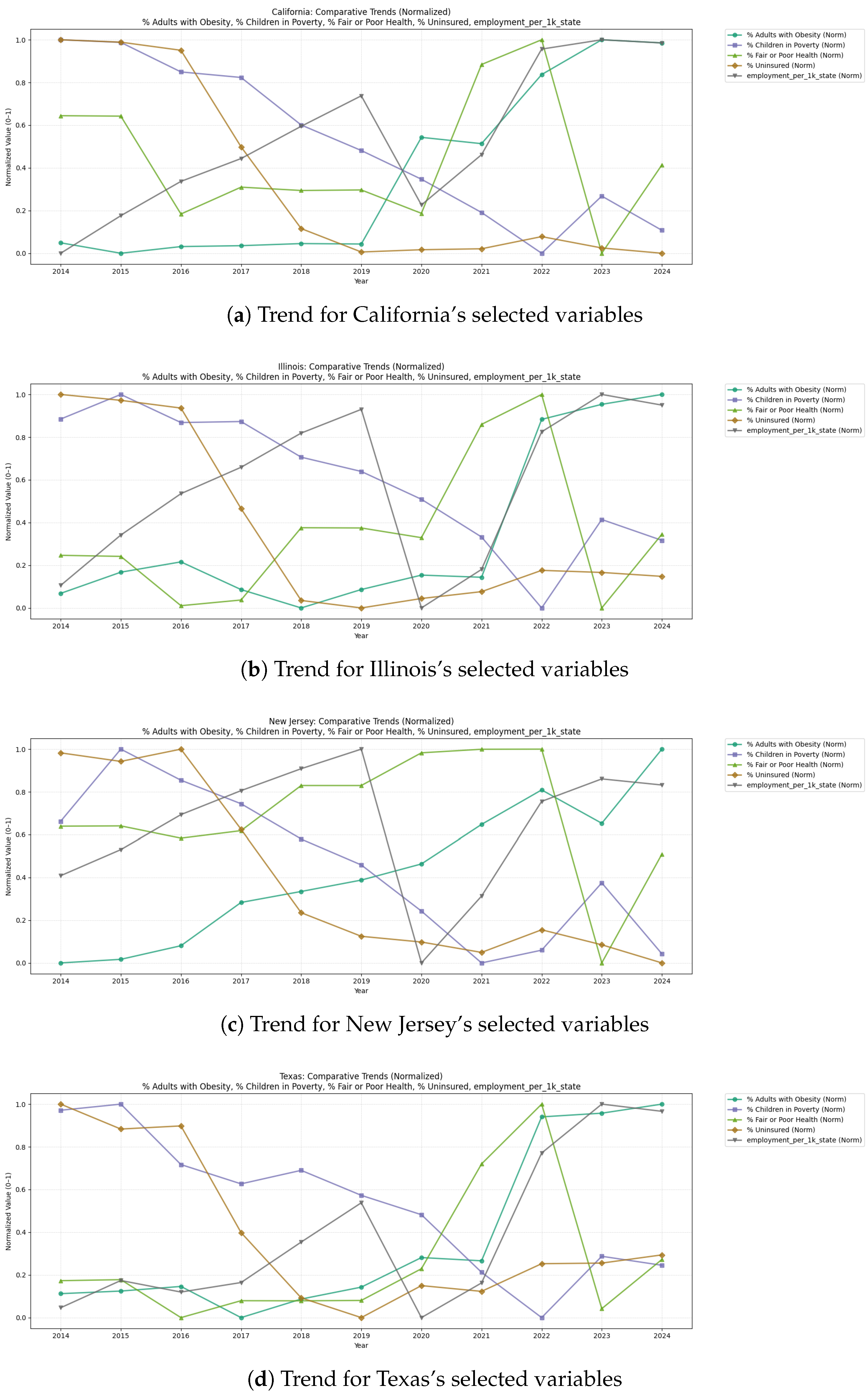
Figure 1. Selected 10–year health, economic and insurance variables’ trend (Normalized).
Computation 14 00022 g001
Figure 2. The distribution of selected variables across US.
Computation 14 00022 g002
Figure 3. Top 10 drivers for employment_per_1k_state for states.
Computation 14 00022 g003
Table 1. XGBoost tuning ranges and final selected hyperparameters (training period only).
ParameterFinal ValueTuning Range
n_estimators800200–1000 (step 50)
learning_rate0.05{0.01, 0.02, 0.03, 0.05, 0.08, 0.10, 0.15}
max_depth52–6
min_child_weight53–15
gamma2.0{0.0, 0.1, 0.5, 1.0, 2.0, 5.0}
subsample0.6{0.5, 0.6, 0.7, 0.8, 0.9}
colsample_bytree0.6{0.5, 0.6, 0.7, 0.8, 0.9}
colsample_bylevel0.5{0.5, 0.6, 0.7, 0.8, 0.9}
reg_alpha0.0{0.0, 0.01, 0.05, 0.1, 0.2, 0.5, 1.0}
reg_lambda2.0{1.0, 2.0, 5.0, 10.0}
Notes: Selection criterion is walk-forward cross-validated RMSE within Years 2019 using an expanding-window design by year. Number of random configurations evaluated: 60. Fixed settings include squared-error objective and histogram tree method.
Table 2. Baseline model performance, state–year panel.
Train (Years ≤ 2019)Test (Years > 2019)
Model R 2 RMSEMAE R 2 RMSEMAE
LASSO0.87546.71434.7740.67572.65452.998
XGBoost (baseline)1.0000.7950.6300.56983.64247.236
MLP0.97022.88916.7690.228111.92689.696
Notes: Errors are measured in units of employment per 1000 residents. Baseline XGBoost and MLP are lightly tuned and exhibit substantial overfitting relative to the linear benchmark.
Table 3. Regularized model and ensemble performance.
Train (Years ≤ 2019)Test (Years > 2019)
Model R 2 RMSEMAE R 2 RMSEMAE
LASSO (regularized)0.87546.82734.8580.67672.52852.838
XGBoost (tuned, regularized)1.0002.2781.0700.80056.96540.097
Random Forest (regularized)0.61082.70536.3590.38999.55057.779
Stacked ensemble (Ridge; OOF meta-train)0.90840.36924.9260.82753.00138.676
Notes: Errors are measured in units of employment per 1000 residents. For the stacked ensemble, the reported “train” metrics correspond to walk-forward OOF predictions within the training period (excluding 2014–2015), rather than in-sample fitted values.
Table 4. Walk-forward out-of-fold (OOF) performance within the training period (Years 2019 ).
ModelOOF Yearsn R OOF 2 RMSE OOF / MAE OOF
Tuned XGBoost (walk-forward OOF)2016–20191970.89942.266/24.558
Stacked ensemble (OOF meta-train)2016–20191970.90840.369/24.926
Notes: OOF predictions are formed by training on years < t and predicting year t. Because this requires prior-year information, the first two training years (2014–2015) do not receive OOF predictions and are excluded from OOF summary statistics.
Table 5. Rolling-origin evaluation for tuned XGBoost (train on years t 1 ; test on year t).
Test Year R 2 RMSEMAE
20180.93931.83822.538
20190.96823.00515.518
20200.81553.18042.198
20210.93829.68122.105
20220.87744.27637.551
20230.81654.32330.799
20240.79061.18634.164
Notes: Rolling-origin evaluation uses an expanding training window and reports year-specific out-of-sample accuracy.
Disclaimer/Publisher’s Note: The statements, opinions and data contained in all publications are solely those of the individual author(s) and contributor(s) and not of MDPI and/or the editor(s). MDPI and/or the editor(s) disclaim responsibility for any injury to people or property resulting from any ideas, methods, instructions or products referred to in the content.