Abstract
Topology optimization (TO) with the variable density concept has made significant advancements in academic research and engineering applications; yet it still encounters obstacles associated with computer inefficiencies in the filtering process. This work introduces a novel filter implementation method that significantly enhances the optimization process by adapting the k-d tree data structure. The proposed method converts traditional neighborhood search operations into extremely efficient spatial searches while preserving solution accuracy. This method inherently accommodates a comprehensive array of manufacturability constraints, including symmetry, local volume control, periodic patterning, stamping-oriented overhang control, and more, without compromising computational duration. Extensive numerical examples validate the proposed method’s efficiency yielding precise, scalable designs, achieving substantial acceleration relative to conventional methods The method demonstrates specific advantage in large scale optimization challenges and intricate complex geometric restrictions, encompassing unstructured meshes. This study explores a new paradigm for effective constraint integration in topology optimization through advanced data structures, providing extensive applicability in engineering design.
1. Introduction
Structural topology optimization (TO) is a potent design methodology that allocates material within a defined design space to either minimize or maximize a given objective function, while conforming to established restrictions for an engineering system. It is widely applied in key industrial fields requiring lightweight, high-performance designs, including aerospace, automotive, renewable energy, and biomedical engineering, which often demand large-scale, high-resolution TO models, making the efficiency of core processes critical to practical implementation. Contemporary TO approaches are often categorized into variable-density or boundary-variation approaches. Prevalent density-based methodologies encompass homogenization [1], solid isotropic material with penalization (SIMP) [2,3,4,5], and evolutionary structural optimization (ESO) [6]. Conversely, boundary-variation methodologies, such as level set method [7,8] and the moving morphable components method [9], have been developed more recently. Each method presents distinct advantages across different domains. Recent solutions amalgamate characteristics from both variable-density and boundary-variation methodologies to improve structural performance. The smooth-edged material distribution approach for topology optimization [10,11,12] produced optimal topologies with smooth boundaries by assigning solid and void element to each element. By combining the level set and SIMP approaches, the level set band concept [13] was able to provide clear border representation.
Checkerboard patterns and mesh dependency are evident in various element-based TO methods [14,15]. Various restrictions have been proposed to address these issues, including the use of high-order elements [16,17], the integration of slope constraints or perimeter controls [18,19], and the implementation of digital image processing technologies [20,21,22,23]. Among these tactics, filtering approaches are essential and have been extensively refined in scholarly study. They can be classified into sensitivity filtering and density filtering. Sensitivity filtering [24], an older heuristic method, was subsequently supplanted by the advancement of density filtering [25], commonly referred to as the two-field projection method. The three-field projection method was subsequently developed to resolve the clarity concerns arising from filtering, providing a more advanced approach to these challenges [26,27]. In TO, the filtering process is often conducted in two stages: first, a neighborhood search to ascertain the adjacent cells of a certain design variable, and subsequently, the calculation of the filtered value through the application of a convolution integral over the found neighbors. The convolution integral averages the filtering variables among adjacent cells, hence smoothing the material distribution. The efficacy of the overall filtering operation is significantly contingent upon the efficiency of the preliminary neighborhood search.
Traditional methods for neighborhood search often rely on brute-force techniques, such as for-loops [28], which examine all design variables, calculate pairwise distances, and identify adjacent elements. While these methods are simple, they become a significant bottleneck in complex problems with high-resolution elements, severely hindering the optimization process. Many researchers have proposed new strategies for more efficient filtering, but each comes with its own set of limitations. For instance, the partial differential equation-based filtering method [29] transforms explicit filters into solutions of additional linear systems. This approach requires substantial computational resources, particularly for large 3D problems. Our k-d tree method avoids this issue by optimizing neighborhood search directly and does not require extra system solvers. Vectorization techniques [30] can speed up convolution operations for structured grids. They are ineffective for irregular geometries or non-uniform meshes due to their reliance on regular memory access patterns. Our method maintains efficiency across both structured and unstructured meshes. This is validated in Section 3.1, Section 3.3, and Section 3.6. Subdomain parallelization [31] enables distributed processing. Its performance is often limited by communication delays between partitions, especially when larger filter radii are used. Our k-d tree reduces data exchange by localizing spatial searches, which complements parallelization. This complementarity is discussed in Section 4. To address these challenges, we propose using a k-d tree (k-dimensional tree) data structure to improve the efficiency of the filtering process, specifically in the neighborhood search phase. This data structure recursively divides the design domain, reducing unnecessary comparisons and speeding up the convolution-based filtering process [32,33]. Our approach preserves the traditional convolution step, ensuring that the core principles of density filtering are maintained. The key innovation of our method lies in its ability to rapidly identify neighboring elements, allowing for more efficient convolution operations without compromising the integrity of the filtered design. Additionally, this approach facilitates the integration of manufacturability constraints through enhanced neighborhood search and sensitivity preprocessing.
The following portions of the paper are structured as outlined below. Section 2 delineates the TO problem statement, followed by the proposed neighborhood search approach employing the k-d tree algorithm, together with its modifications for symmetry constraints and implicit local volume constraints, thereby offering a scalable framework for more extensive manufacturability requirements. Section 3 substantiates the techniques with five numerical examples and an engineering application, illustrating their efficacy and adaptability. The concluding section delineates the findings.
2. Topology Optimization Problem Statement
2.1. Problem Formulation
In a design domain comprising NE finite elements, the objective is to maximize stiffness while conforming to a certain volume fraction constraint. The TO formulation for the continuum structure is formally expressed as follows:
where vector consists of the design variables exclusively pertinent to each element; The static compliance c quantifies structural stiffness, while represents the global stiffness matrix. The symbols and denote the displacement and external load vector, respectively. and are the total material volume and permissible volume, respectively. The variable denotes the specified volume fraction.
2.2. Material Interpolation with Three-Phase SIMP Method
The SIMP model is commonly utilized to interpolate material properties between solid and void states [34]. The Young’s modulus, denoted as , is defined as:
where and represent the Young’s modulus of the solid material and to void phase, respectively. The penalty factor generally satisfied the inequality .
It is noteworthy that Equation (2) employs physical density, which is utilized in finite element analyses and volume computations, and possesses authentic physical relevance. The physical density values are generated at the results’ post-processing phase. Conversely, the symbol in Equation (1) functions as a design variable and lacks substantial physical significance.
2.3. Filtering and Threshold Projection
In the three-field SIMP approach, a mapping relationship exists between the design variable to the physical density , incorporating the filtered density . As previously discussed, filtering techniques are employed to avert numerical instabilities, including checkerboard patterns and mesh dependency. The mathematical relationship between the design variable and the filtered density can be given by:
where represents a sphere in three dimensions or a circle in two dimensions, centered at with a radius of . is the distance from unit to the center of unit , where is the element in the domain ; The weighting factor is mathematically expressed as
Threshold projection techniques, such as the Heaviside projection, are employed to achieve clearly defined structural boundaries. These methods map the filtered density field onto a physical density field, ensuring a distinct transition between solid and void regions. The Heaviside projection can be defined as [27,35]:
where is a parameter that regulates the sharpness of the projection, and is a threshold with values ranging from 0 to 1. As the projection parameter escalates, the filtered density values converge towards 0 and 1. In practical application, a strategy of gradually increasing the parameter is typically employed to achieve completely distinct topologies. Figure 1 shows the schematic of topology optimization.
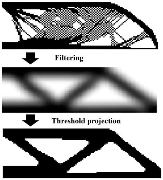
Figure 1.
The schematic of topology optimization.
2.4. Sensitivity Analysis
For the compliance minimization problem, the sensitivity of the compliance c with respect to the physical density can be expressed as follows:
where represents the element displacement vector. denotes the stiffness matrix of solid material. This information is crucial for the TO algorithm to navigate the design space towards an optimal solution.
The sensitivity of the static compliance can be conducted using the chain rule as
where denotes the derivative of the static compliance with respect to the e-th design variable.
2.5. Neighborhood Search Based on k-d Tree Algorithm
A k-d tree is formed by iteratively dividing the dataset into two subsets until each subset includes either a single data point or none. Let the coordinates of all m elements constitute a three-dimensional point set λ = {λ1, λ2, …, λm}, where each point λi is represented by the three-dimensional vector λi = (λix, λiy, λiz). This study uses the dimension with the greatest variation as the splitting axis for generating the tree structure incrementally, to maximize tree balance and enhance query efficiency, given the random distribution of element coordinates in practical applications. The precise computations are as follows:
where d represents the dimension, with its value being (i.e., the x, y, z axes), λid denotes the value of the vector λi in the d-th dimension, represents the mean value in the d-th dimension, and represents the variance in the d-th dimension.
Identify the dimension exhibiting the greatest variance to serve as the splitting axis, and arrange all points based on the d-th dimension.
Determine the median, which serves as the splitting point of the current node, segmenting the point set λ into two subsets:
where Md denotes the median value in the d-th dimension, λl and λr signify the subsets of points contained are at the left and right subtrees of the splitting point, respectively. Recursively repeat the above steps for λl and λr until each subset contains either a single point or none.
The k-d tree constructed can facilitate efficient range queries. To identify all points within a radius of r surrounding a given query point λj = (λjx, λjy, λjz), the computation procedure is as follows:
where represents the Euclidean distance between the query point λj and the current tree node λt = (λtx, λty, λtz). If it satisfies Equation (14), the current tree node λt is incorporated into the result set.
Assume that the query point and the current tree node in the splitting dimension have values of λjd and λtd, respectively, and that the splitting dimension is d. The recursive criteria are as follows:
If Equation (15) holds, it signifies that the query neighborhood intersects with the search space of the left subtree, prompting the algorithm recurses into the left subtree. If Equation (16) is satisfied, it indicates that the query neighborhood intersects with the search space of the right subtree, so the algorithm recurses into the right subtree. Repeat the aforementioned process until the current tree node has no subtrees. The processes for constructing a k-d tree and conducting neighborhood searches are outlined in pseudocode as Algorithm 1: Construction of k-d Tree and Neighborhood Search.
| Algorithm 1: Construction of k-d Tree and Neighborhood Search |
|
A k-d tree recursively divides the space into smaller areas, enabling each node’s examination to concentrate solely on a particular subspace rather than the entire space. If the query point is distant from the current node’s splitting position, the subtree may be disregarded, significantly decreasing the number of nodes that need assessment. Utilizing brute-force methods like nested for-loops requires comparing each point, resulting in a time complexity of O(n2), which is exceedingly wasteful for large data searches. In contrast, the ideal time complexity for a k-d tree search is O(logn), and even in the worst-case scenario, its performance far surpasses O(n2). Chapter 3 will provide numerical examples to assess the effectiveness of these two strategies.
2.6. The Extension of Neighborhood Search with k-d Tree
Manufacturability constraints in engineering applications encompass a wide spectrum of requirements, including but not limited to planar symmetry, rotational symmetry, local volume control, periodic patterning, stamping-oriented overhang control [36,37,38,39,40]. This section specifically examines planar symmetry, rotational symmetry (shown in Figure 2) and implicit local volume constraint as representative cases, developing corresponding heuristic formulations to demonstrate the method’s core capability. Notably, the proposed k-d tree method can be readily extended to implement virtually all other types of symmetry constraints without fundamental algorithmic modifications.
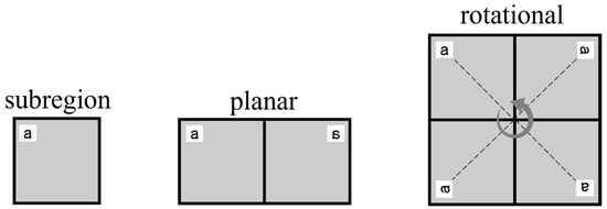
Figure 2.
Planar symmetry and rotational symmetry.
2.6.1. Planar Symmetry
Suppose that the design domain is divided into j symmetric sets, and the sensitivity of symmetric elements in each set is averaged, it yields
where is the sensitivity of element i in the jth symmetric set, is the sensitivity of each element and its symmetric elements after considering symmetry constraints. This sensitivity updating process is illustrated in Figure 3.
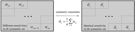
Figure 3.
The sensitivity updating process after applying symmetric constraints.
For the planar symmetry constraint, without losing generality, take the planar yoz pair as an example. For an element along coordinates λi = (xi, yi, zi), its symmetric counterpart satisfies:
In implementation, we enforce symmetry by taking the absolute value of the x-coordinate, thus symmetric coordinates λi and λis will map to the same modified coordinate:
Assume that S = {λ1*, λ1s*, λ2*, λ2s*, … λn*, λns*} is the set of all modified element coordinates. For a given tolerance ε > 0, the k-d tree algorithm identifies symmetric element pairs or groups such that
where represents the Euclidean distance between any two points λu and λv in the set S. It is significant that Equation (20) nearly parallels Equation (14), varying in the substitution of the radius r with a tolerance ε approaching zero. This update ingeniously alters the function of the k-d tree from looking for items within a radius r to identifying symmetrically positioned elements located at the same coordinates. The parameter ε is set to 0.01 times the average element size for regular meshes because symmetric elements in such meshes have uniform spacing equal to the element size—this small tolerance ensures only true symmetric pairs are detected, avoiding false matches from non-symmetric elements. For irregular meshes, element dimensions and spacing vary, so ε is increased to 0.2 times the average element size to accommodate minor coordinate deviations from discretization while still preventing missed symmetric pairs. This choice of ε aligns with the geometric characteristics of the respective mesh types, ensuring symmetry enforcement remains accurate without relying on arbitrary heuristics.
Notably, the consistency of optimized results across regular and irregular meshes (Section 3.1 and Section 3.3) further supports the appropriateness of ε: in both cases, the final topologies exhibit clear symmetry and stable compliance values, confirming that the selected ε does not introduce numerical inconsistencies or compromise design quality.
2.6.2. Rotational Symmetry
For the rotational symmetry constraint, the Cartesian coordinates (x, y, z) at the center of the element are first converted into spherical polar coordinates (rp, θ, φ), i.e.,
where the radial distance is the distance from the coordinate point to the center of the sphere o, the polar angle θ is the angle between the z axis and , and the azimuth angle φ is the angle between the projection line of onto the xoy plane and the positive direction of the x axis.
Considering the rotational symmetry number n, the azimuth angle increment for each symmetric subregion is
Consequently, the symmetric element group under this constraint has the following characteristics: The radial distance r and the polar angle θ remain constant, and for the kth symmetric subregion, the azimuth angle is
where is the initial azimuth angle. The elements with a φ value in each subregion are traversed by the programming language, corresponding to the reduced angle , ensuring that elements under symmetric restrictions are overlapped. Then Equation (20) is used to search for symmetric elements.
2.6.3. Implicit Local Volume Constraint
The suggested filtering technique may also be utilized in the construction of porous structures via the implicit local volume constraint [38]. As illustrated in Figure 4, the primary concept is to prevent the accumulation of material regions by incorporating voids in the physical density.
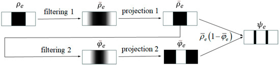
Figure 4.
The implementation principle of implicit local volume constraints.
The updated physical density field is computed by performing a point-wise multiplication of the two projected fields.
where is the second projected field. The point-by-point multiplication of two scalar fields facilitates material distribution without violating the local volume limit, and the updated physical density can be incorporated into Equation (2) for material interpolation and stiffness matrix computation.
Similar to Equation (3), the second filtered field characterizes the local volume fraction of solid material in the scalar field , it yields
where denotes the neighborhood set of the element e for the second filter and denotes the number of elements in the set. Here, is defined in the same way as in Equation (1) except r replaced with R, which is usually larger than that of r.
The second projected field is constructed by applying a novel projection function to the previously obtained filtered field , expressed as:
where represents a parameter controlling the sharpness of the second projection, is the second filtered filed. The parameter term of this formula closely resembles the initial projection function in Equation (5); however, the second projection solely elevates the lesser value to 1, resulting in the aforementioned projection function demonstrating a low-pass characteristic, which is precisely contrary to the outcome of the step projection function in Equation (5).
The ensuing optimization solution is congruent with the aforementioned strategy. In assessing sensitivity, it is crucial to acknowledge that the incorporation of the second filtering and projection techniques requires the inclusion of these two factors in the chain derivation formula referenced in Equation (7).
This method necessitates two neighborhood searches due to the two filter radii, with the second search encompassing a larger range than the first. This complexity may pose challenges for large-scale applications. The k-d tree algorithm proposed in this work efficiently performs both neighborhood searches, hence improving the efficiency of addressing porous structure issues.
3. Numerical Examples and Discussion
In the absence of contrary indications, an elastic modulus of 1 and a Poisson’s ratio of 0.3 are assigned, respectively. The convention TO problem, as articulated in Equation (1), can be addressed through moving morphable asymptotes (MMA) technique [41]. A supplementary parameter for the movement limit is established at 0.05. Due to the establishment of low thresholds for convergence criteria, the optimizations conducted in Section 3 consistently concluded upon reaching the maximum of 350 iterations. β commences at a value of 1 and doubles at every 50 steps until it reaches a maximum of 64. All numerical tests are conducted on a desktop computer using an Intel i7 2.93 GHz CPU and 64 GB of RAM.
3.1. Example 1
The benchmark Messerschmitt–Bölkow–Blohm (MBB) structure as depicted in Figure 5, with a design domain measuring 120 × 40, is optimized to validate the efficacy of the proposed k-d tree density filtering technique. The design realm was discretized into regular elements of dimensions 120 × 40, 240 × 80, 360 × 120, and 480 × 160, respectively. The left boundary is fully constrained in the horizontal direction, while vertical support is applied at the bottom-right corner. A vertical force F = 1 is exerted at the upper left corner. The target volume fraction and the filter radius r is set to 50% and 5, respectively.
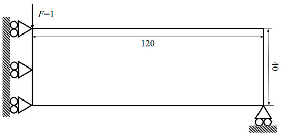
Figure 5.
Design domain of MBB structure.
No checkerboard patterns are present in any of the optimized topologies, hence validating the efficacy of the utilized filtering method in eliminating such numerical aberrations. The above Figure 6 depicts the outcomes obtained from the proposed density filtering method. The study of these data demonstrates a strong consistency in various optimized topologies across different mesh densities, signifying the efficacy of the proposed strategy in attaining mesh-independent solutions. The compliance values of the final design show a slight upward trend with higher element resolution. This is expected, as finer discretization captures more intricate structural details, which can result in higher compliance values.
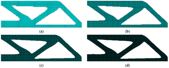
Figure 6.
Optimized structures were obtained by (a) 120 × 40 elements, c = 228.345, (b) 240 × 80 elements, c = 229.803, (c) 360 × 120 elements, c = 232.363 and (d) 480 × 160 elements, c = 234.799.
3.2. Example 2
This example optimizes a 3D L-shaped structure, aiming to validate the advantages of the k-d tree search algorithm over the traditional brute-force search algorithms. The structure is clamped at its top edge and a concentrated force F = 0.1 is exerted on the upper sideline of the right side, as illustrated in Figure 7a. The design domain is discretized using brick elements with elemental sizes of 2, 1, and 0.5, resulting in total elemental counts of 2500, 20,000, and 160,000, respectively. The desired volume fraction is set to 50%. Table 1 shows the computation times spent in neighborhood search and overall optimization between the brute-force and k-d tree algorithms.
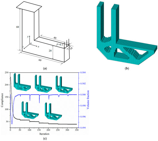
Figure 7.
Optimization of the L-shaped structure. (a) loading and boundary conditions, (b) optimized design, and (c) iteration histories of compliance and volume fraction.

Table 1.
Computation times spent in neighborhood search and overall optimization between the brute-force and k-d tree algorithms.
Both the k-d tree and brute-force search approaches follow the same iterative processes and yield the same results, with the only difference being computational efficiency. The optimization problem is addressed inside the same hardware environment to guarantee that the comparison of algorithm efficiency remains unaffected by hardware discrepancies. Using the model with 20,000 elements as an example, its topological optimization results and iteration histories are depicted in Figure 7b and Figure 7c, respectively. The graph illustrates compliance as a stepwise sequence of possessive decline. The parameter β updates every 50 steps, resulting in a sudden drop followed by a plateau until the subsequent update. This procedure demonstrates the effect of progressively augmenting the beta value to enhance material configuration. The volume is consistently controlled within the volume fraction.
Table 1 demonstrates that k-d tree algorithms significantly outperform the brute-force method in computational efficiency, particularly as the number of elements increases. For a limited number of elements (2500 elements), both methodologies are feasible. Nonetheless, the k-d tree demonstrates a significant speed advantage. As the element count increases to 20,000, the k-d tree maintains its efficiency, decreasing both neighborhood search time and overall optimization time compared to the brute-force method. As the element count nears 160,000, the brute-force method becomes impractical due to memory constraints; however, the k-d tree continues to exhibit efficient performance. This underscores the scalability of the k-d tree technique and its adeptness efficiently addressing large-scale optimization problems. Thus, the increasing computational efficiency of k-d tree makes them a preferable choice for intricate, large-scale applications, whereas conventional methods are inadequate.
3.3. Example 3
This example features a double L-shaped structure, intended to demonstrate the proposed approach’s capability to attain a planar symmetry design, despite the presence of irregular elements. The design domain is discretized utilizing quadrilateral and triangular elements; each elemental size is 1, respectively. The boundary conditions are depicted in Figure 8, illustrate the combination of two L-shaped beams, fixed at the top, subject to vertical downward loads of magnitude 1 applied to the left and right corners. Additionally, a horizontal leftward load of magnitude 0.3 is applied to the left corner to introduce asymmetry in the topology optimization results. The target volume fraction and the filter radius r are set to 50% and 3, respectively. Figure 9 illustrates various optimized topologies prior to and subsequent to the implementation of the planar symmetry constraint.
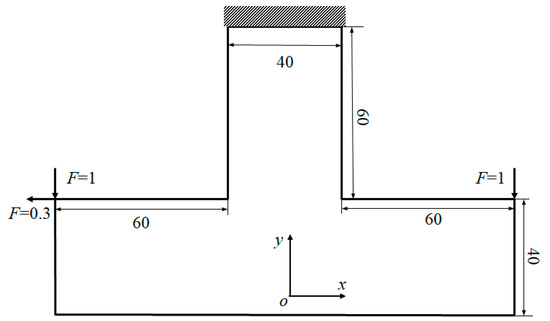
Figure 8.
Design domain of double L-shaped structure.
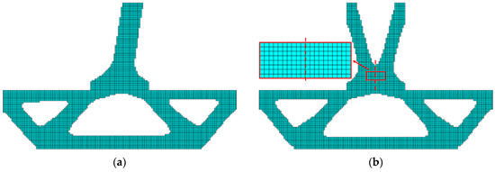
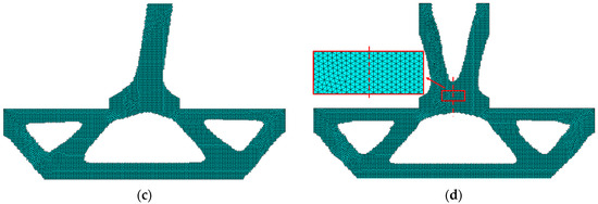
Figure 9.
Optimized structures were obtained by (a) regular elements without planar symmetry constrained, (b) regular elements with planar symmetry constraint, (c) irregular elements without planar symmetry constrained and (d) irregular elements with planar symmetry constraint.
3.4. Example 4
This example depicts a gear design featuring a circular shaped design domain and non-designable inner- and outer-rings, aiming to validate the rotational symmetry design using the proposed approach. The blue-designated region is attached to the white non-designable area. The boundary conditions are depicted in Figure 10. A concentrated force of magnitude 1 is exerted tangentially along the outside circumference as surface traction. The inner bearing of the inner ring is fully restricted. The target volume percentage is established at 50%, with the filter radius set at 4. When the rotational symmetry number is designated as n, the optimized material distribution results are illustrated in Figure 11.
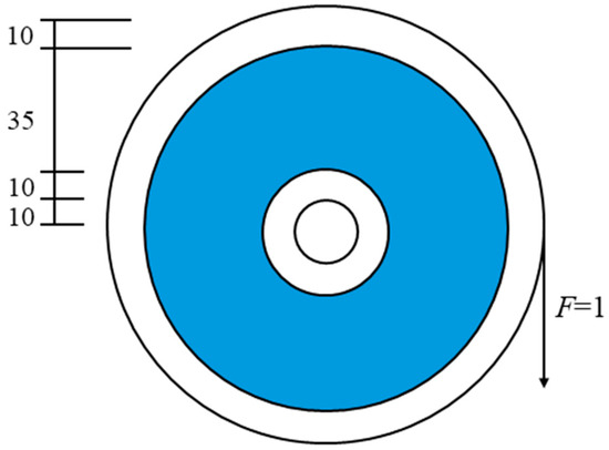
Figure 10.
The design domain and the boundary conditions.
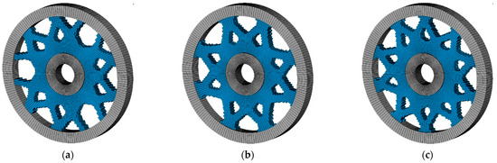
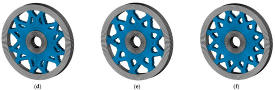
Figure 11.
The optimized topologies with various numbers of circumferential cycles (a) n = 3, c = 136.55, (b) n = 4, c = 136.46, (c) n = 5, c = 142.94 (d) n = 6, c = 144.32 (e) n = 9, c = 157.44 and (f) n = 12, c = 178.23.
Figure 11 demonstrates that the application of rotational symmetry as an additional constraint in the optimization problem generally diminishes the structure’s performance. When the cycle count is low, the constraint effect is nuanced, seen only in modifications to the topological pattern. As the quantity escalates, the rotational symmetry requirement becomes paramount in the optimization problem, affecting both performance and the ultimate topology. The structure achieves the limitation by compromising rigidity, leading to an increase in compliance. Through coordinate translation, the k-d tree can convert the symmetric constraint problem into a defined neighborhood search problem, hence enabling the implementation of circumferential constraints. The numerical findings underscore the efficacy of the proposed method in addressing rotational symmetry constraints.
3.5. Example 5
A 2D bone-like structure was optimized to assess the viability of the local volume fraction approach augmented by the proposed k-d tree algorithm [42]. The finite element model comprises 29,854 elements and 29,792 nodes, with three layers of elements kept as the non-design domain. The bottom edge was entirely fixed, while concentrated loads were applied at both top corners with a downward 45° inclination (θ = 45°), as depicted in Figure 12. The magnitude of the left and right load . Set the volume fraction to 0.5 and the maximum number of iteration steps to 350. Specify the filter parameters r = 4.5 and R = 10, the projection parameters β1 = 1 and β2 = 8, and the projection parameters η1 = 0.5 and η2 = 0.6. The optimized infill structure is drawn in Figure 13.
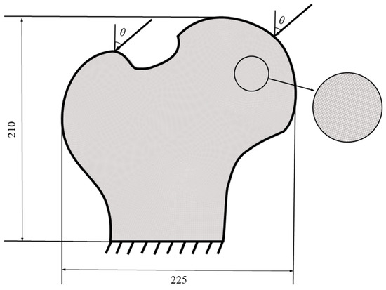
Figure 12.
The boundary conditions of the bone-like structure.
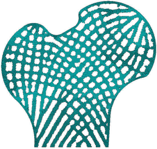
Figure 13.
The optimized bone-like structure.
As expected, a porous structure is generated to satisfy the given design criteria, while all constraints are nearly rigorously fulfilled. This challenge requires the implementation of two neighborhood searches with radius r and R need to be implemented. The k-d tree technique can accurately execute two neighborhood searches, which usually demand considerable time using traditional techniques. Additionally, the results demonstrate the k-d tree algorithm’s practicality under the local volume constraint.
3.6. Engineering Application
In recent years, structural optimization technology has gained prominence in the wind power industry. TO method serves as an innovative design tool during the conceptual design phase, as evidenced in the structural design of blades [43,44], jackets [45,46,47] and tripod supports [48]. This example demonstrates the TO of the front framework of a wind turbine validate the feasibility and superiority of the k-d tree algorithm for large-scale engineering challenges. The finite element of assembly model comprises 764,477 nodes and 824,573 elements, in which the front framework is predominately discretized using hexahedral solid elements. Figure 14 illustrates the finite element model of the assembly. The material possesses an elastic modulus of 169,000 MPa and a Poisson’s ratio of 0.275. The target volume fraction is specified as 40%. This study investigates the weighed combination of moments in the y and z directions, specifically My and Mz. The resultant topology is plotted in Figure 15.
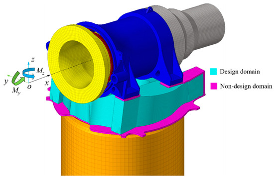
Figure 14.
The finite element model of the assembly.
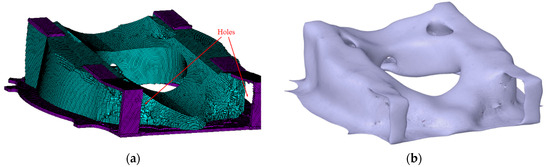
Figure 15.
The optimized front framework (a) finite element model and (b) STL model after smoothing process.
Figure 15 illustrates that, under the loading conditions influenced by moments My and Mz, the material distribution from the apex of the tower via the rear bearing seat establishes a clear force transmission channel at the rear end of the front structure. The apparent holes in the rear area suggest that these regions are ineffective or erroneous. The implementation of the k-d tree algorithm to compute the aforementioned model on a standard office computer (Intel i7 2.93 GHz CPU, 64 GB RAM) required approximately 2.5 h for completion, whereas previously, complex models of this magnitude typically necessitated cloud computing platforms or supercomputers, where more time is required for processing. This engineering application demonstrates that the k-d tree technique can swiftly and effectively handle complex geometric shapes and extensive datasets, a task that was difficult in previous topology optimization studies.
4. Conclusions
This study has presented an efficient filtering method for structural TO utilizing the k-d tree data structure, applicable for addressing practical manufacturability restrictions. The use of the k-d tree algorithm obviates the necessity for laborious repetitive examinations and offers a scalable solution for large-scale optimization challenges, where conventional methods would falter under computing demands.
Numerical examples demonstrate that the proposed filtering approach successfully eradicates checkerboard patterns while preserving robust performance across diverse mesh densities. The k-d tree algorithm demonstrates remarkable advantages over traditional brute-force techniques, particularly for large-scale problems. Furthermore, the approach precisely enforces constraints even with irregular elements through adaptive tolerance adjustment. The algorithm addresses symmetry constraints using coordinate transformation and satisfies local volume constraints through multiple neighborhood searches. Although this study exemplifies only these two types of constraints, the proposed framework can be readily extended to other manufacturability constraints via the same efficient spatial query mechanism. The industrial case study further confirms the method’s practical value. It reduces the optimization runtime of large structural components such as wind turbine frameworks from over 8 h to around 2.5 h and enables optimized structures to achieve 20 percent weight reduction while maintaining 7.7 percent higher stiffness. This directly lowers manufacturing hardware costs for enterprises and supports lightweight high-performance design goals in engineering practice.
Future works will focus on three key points. First, optimize the k-d tree’s recursive partitioning logic to adapt to 3D models with irregular curved boundaries common in large wind turbine components. Second, integrate the method with additive manufacturing constraints such as overhang angle limits to expand its application scope in wind turbine part manufacturing. Third develop a lightweight version of the algorithm compatible with edge computing devices for on-site real time optimization in wind turbine component production workshops.
Author Contributions
J.H.: validation and software, methodology; A.S.: validation and software, methodology, revision; K.L.: conceptualization, methodology, writing—original draft preparation and revision; Y.C.: writing and editing; R.G.: writing and editing; J.J.: writing—reviewing and editing; T.T.: writing—reviewing and editing. All authors have read and agreed to the published version of the manuscript.
Funding
This work was financially supported by the National Key Research and Development Program of China (No. 2024YFE0208600), the National Natural Science Foundation of China (No. U24B2090), the Fundamental Research Funds for the Central Universities (No. 2024JC006).
Data Availability Statement
The data presented in this study are available on request from the corresponding author.
Conflicts of Interest
Author Tao Tao was employed by China Southern Power Grid Technology Co., Ltd. The remaining authors declare that the research was conducted in the absence of any commercial or financial relationships that could be construed as a potential conflict of interest.
References
- Bendsøe, M.P.; Kikuchi, N. Generating optimal topologies in structural design using a homogenization method. Comput. Methods Appl. Mech. Eng. 1988, 71, 197–224. [Google Scholar] [CrossRef]
- Bendsøe, M.P. Optimal shape design as a material distribution problem. Struct. Optim. 1989, 1, 193–202. [Google Scholar] [CrossRef]
- Bendsøe, M.P.; Sigmund, O. Material interpolation schemes in topology optimization. Arch. Appl. Mech. 1999, 69, 635–654. [Google Scholar] [CrossRef]
- Zhou, M.; Rozvany, G.I.N. The COC algorithm, part II: Topological, geometrical and generalized shape optimization. Comput. Methods Appl. Mech. Eng. 1991, 89, 309–336. [Google Scholar] [CrossRef]
- Long, K.; Wang, X.; Gu, X. Local optimum in multi-material topology optimization and solution by reciprocal variables. Struct. Multidiscip. Optim. 2018, 57, 1283–1295. [Google Scholar] [CrossRef]
- Xie, Y.M.; Steven, G.P. A simple evolutionary procedure for structural optimization. Comput. Struct. 1993, 49, 885–896. [Google Scholar] [CrossRef]
- Allaire, G.; Jouve, F.; Toader, A.M. Structural optimization using sensitivity analysis and a level-set method. J. Comput. Phys. 2004, 194, 363–393. [Google Scholar] [CrossRef]
- Wang, M.Y.; Wang, X.; Guo, D. A level set method for structural topology optimization. Comput. Methods Appl. Mech. Eng. 2003, 192, 227–246. [Google Scholar] [CrossRef]
- Guo, X.; Zhang, W.; Zhong, W. Doing topology optimization explicitly and geometrically—A new moving morphable components based framework. J. Appl. Mech. 2014, 81, 081009. [Google Scholar] [CrossRef]
- Fu, Y.F.; Rolfe, B.; Chiu, L.N.S.; Wang, Y.; Huang, X.; Ghabraie, K. SEMDOT: Smooth-edged material distribution for optimizing topology algorithm. Adv. Eng. Softw. 2020, 150, 102921. [Google Scholar] [CrossRef]
- Fu, Y.F.; Rolfe, B.; Chiu, L.N.S.; Wang, Y.; Huang, X.; Ghabraie, K. Smooth topological design of 3D continuum structures using elemental volume fractions. Comput. Struct. 2020, 231, 106213. [Google Scholar] [CrossRef]
- Fu, Y.F.; Long, K.; Rolfe, B. On non-penalization SEMDOT using discrete variable sensitivities. J. Optim. Theory Appl. 2023, 198, 644–677. [Google Scholar] [CrossRef]
- Wei, P. Level set band method: A combination of density-based and level set methods for the topology optimization of continuums. Front. Mech. Eng. 2020, 15, 390–405. [Google Scholar] [CrossRef]
- Sigmund, O.; Petersson, J. Numerical instabilities in topology optimization: A survey on procedures dealing with checkerboards, mesh-dependencies and local minima. Struct. Optim. 1998, 16, 68–75. [Google Scholar] [CrossRef]
- Zhou, M.; Shyy, Y.K.; Thomas, H.L. Checkerboard and minimum member size control in topology optimization. Struct. Multidiscip. Optim. 2001, 21, 152–158. [Google Scholar] [CrossRef]
- Diaz, A.; Sigmund, O. Checkerboard patterns in layout optimization. Struct. Optim. 1995, 10, 40–45. [Google Scholar] [CrossRef]
- Poulsen, T.A. A simple scheme to prevent checkerboard patterns and one-node connected hinges in topology optimization. Struct. Multidiscip. Optim. 2002, 24, 396–399. [Google Scholar] [CrossRef]
- Haber, R.B.; Jog, C.S.; Bendsøe, M.P. A new approach to variable-topology shape design using a constraint on perimeter. Struct. Optim. 1996, 11, 1–2. [Google Scholar] [CrossRef]
- Petersson, J.; Sigmund, O. Slope constrained topology optimization. Int. J. Numer. Methods Eng. 1998, 41, 1417–1434. [Google Scholar] [CrossRef]
- Sigmund, O. Morthology-based black and white filters for topology optimization. Struct. Multidiscip. Optim. 2007, 33, 401–424. [Google Scholar] [CrossRef]
- Bourdin, B. Filters in topology optimization. Int. J. Numer. Methods Eng. 2001, 50, 2143–2158. [Google Scholar] [CrossRef]
- Groenwold, A.A.; Etman, L.F. A simple heuristic for gray-scale suppression in optimality criterion-based topology optimization. Struct. Multidiscip. Optim. 2009, 39, 217–225. [Google Scholar] [CrossRef]
- Wang, M.Y.; Wang, S. Bilateral filtering for structural topology optimization. Int. J. Numer. Methods Eng. 2005, 63, 1911–1938. [Google Scholar] [CrossRef]
- Sigmund, O.; Maute, K. Sensitivity filtering from a continuum mechanics perspective. Struct. Multidiscip. Optim. 2012, 46, 471–475. [Google Scholar] [CrossRef]
- Bruns, T.E.; Tortorelli, D.A. Topology optimization of non-linear elastic structures and compliant mechanisms. Comput. Methods Appl. Mech. Eng. 2001, 190, 3443–3459. [Google Scholar] [CrossRef]
- Guest, J.K.; Prévost, J.H.; Belytschko, T. Achieving minimum length scale in topology optimization using nodal design variables and projection functions. Int. J. Numer. Methods Eng. 2004, 61, 238–254. [Google Scholar] [CrossRef]
- Wang, F.; Lazarov, B.S.; Sigmund, O. On projection methods, convergence and robust formulations in topology optimization. Struct. Multidiscip. Optim. 2011, 43, 767–784. [Google Scholar] [CrossRef]
- Sigmund, O. A 99 line topology optimization code written in Matlab. Struct. Multidiscip. Optim. 2001, 21, 120–127. [Google Scholar] [CrossRef]
- Lazarov, B.S.; Sigmund, O. Filters in topology optimization based on Helmholtz-type differential equations. Int. J. Numer. Methods Eng. 2011, 86, 765–781. [Google Scholar] [CrossRef]
- Andreassen, E.; Clausen, A.; Schevenels, M.; Lazarov, B.S.; Sigmund, O. Efficient topology optimization in MATLAB using 88 lines of code. Struct. Multidiscip. Optim. 2011, 43, 1–6. [Google Scholar] [CrossRef]
- Zhao, Z.L.; Rong, Y.; Yan, Y.; Feng, X.Q.; Xie, Y.M. A subdomain-based parallel strategy for structural topology optimization. Acta Mech. Sin. 2023, 39, 422357. [Google Scholar] [CrossRef]
- Foley, T.; Sugerman, J. KD-tree acceleration structures for a GPU raytracer. In Proceedings of the ACM SIGGRAPH/EUROGRAPHICS Conference on Graphics Hardware, Los Angeles, CA, USA, 30–31 July 2005; pp. 15–22. [Google Scholar]
- Narasimhulu, Y.; Suthar, A.; Pasunuri, R.; Vadlamudi, C.V. CKD-Tree: An Improved KD-Tree Construction Algorithm. In Proceedings of the ISIC2021: International Semantic Intelligence Conference, New Delhi, India, 25–27 February 2021; pp. 211–218. Available online: https://ceur-ws.org/Vol-2786/Paper28.pdf (accessed on 15 March 2024).
- Rozvany, G.I. A critical review of established methods of structural topology optimization. Struct. Multidiscip. Optim. 2009, 37, 217–237. [Google Scholar] [CrossRef]
- Li, Q.; Liang, G.; Luo, Y.; Zhang, F.; Liu, S. An explicit formulation for minimum length scale control in density-based topology optimization. Comput. Methods Appl. Mech. Eng. 2023, 404, 115761. [Google Scholar] [CrossRef]
- Liu, Y.; Li, Z.; Wei, P.; Wang, W. Parameterized level-set based topology optimization method considering symmetry and pattern repetition constraints. Comput. Methods Appl. Mech. Eng. 2018, 340, 1079–1101. [Google Scholar] [CrossRef]
- Zuo, Z.H.; Xie, Y.M.; Huang, X. Optimal topological design of periodic structures for natural frequencies. J. Struct. Eng. 2011, 137, 1229–1240. [Google Scholar] [CrossRef]
- Dou, S. A projection approach for topology optimization of porous structures through implicit local volume control. Struct. Multidiscip. Optim. 2020, 62, 835–850. [Google Scholar] [CrossRef]
- Zuo, Z.H.; Huang, X.; Yang, X.; Rong, J.H.; Xie, Y.M. Comparing optimal material microstructures with optimal periodic structures. Comput. Mater. Sci. 2013, 69, 137–147. [Google Scholar] [CrossRef]
- Huang, X.; Xie, Y.M. Optimal design of periodic structures using evolutionary topology optimization. Struct. Multidiscip. Optim. 2008, 36, 597–606. [Google Scholar] [CrossRef]
- Svanberg, K. The method of moving asymptotes—A new method for structural optimization. Int. J. Numer. Methods Eng. 1987, 24, 359–373. [Google Scholar] [CrossRef]
- Wu, J.; Aage, N.; Westermann, R.; Sigmund, O. Infill optimization for additive manufacturing—Approaching bone-like porous structures. IEEE Trans. Vis. Comput. Graph. 2017, 24, 1127–1140. [Google Scholar] [CrossRef]
- Alkebsi, E.A.; Ameddah, H.; Outtas, T.; Almutawakel, A. Design of graded lattice structures in turbine blades using topology optimization. Int. J. Comput. Integr. Manuf. 2021, 34, 370–384. [Google Scholar] [CrossRef]
- Stanford, B.; Beran, P.; Bhatia, M. Aeroelastic topology optimization of blade-stiffened panels. J. Aircr. 2014, 51, 938–944. [Google Scholar] [CrossRef]
- Zhang, C.; Long, K.; Zhang, J.; Lu, F.; Bai, X.; Jia, J. A topology optimization methodology for the offshore wind turbine jacket structure in the concept phase. Ocean Eng. 2022, 266, 112974. [Google Scholar] [CrossRef]
- Lan, R.; Long, K.; Saeed, A.; Geng, R.; Chen, Y.; Zhang, J.; Tao, T.; Liu, J. Fail-safe topology optimization for a four-leg jacket structure of offshore wind turbines. Structures 2024, 62, 106183. [Google Scholar] [CrossRef]
- Zhou, Y.; Zhang, J.; Long, K.; Saeed, A.; Tao, T.; Chen, J. Topology optimization on a jacket structure for offshore wind turbines by altering structural design domain. Appl. Ocean Res. 2025, 154, 104421. [Google Scholar] [CrossRef]
- Lu, F.; Long, K.; Zhang, C.; Zhang, J.; Tao, T. A novel design of the offshore wind turbine tripod structure using topology optimization methodology. Ocean Eng. 2023, 280, 114607. [Google Scholar] [CrossRef]
Disclaimer/Publisher’s Note: The statements, opinions and data contained in all publications are solely those of the individual author(s) and contributor(s) and not of MDPI and/or the editor(s). MDPI and/or the editor(s) disclaim responsibility for any injury to people or property resulting from any ideas, methods, instructions or products referred to in the content. |
© 2025 by the authors. Licensee MDPI, Basel, Switzerland. This article is an open access article distributed under the terms and conditions of the Creative Commons Attribution (CC BY) license (https://creativecommons.org/licenses/by/4.0/).