Abstract
This paper presents a comprehensive study of nonlinear wave and oscillator dynamics under both deterministic and stochastic influences. By comparing soliton-like and dispersive waveforms, we employ spectral solvers, Darboux transformations, and nonlinear diagnostics, including Lyapunov exponents, power spectral analysis, and multidimensional phase-space reconstructions, to examine transitions from quasiperiodic motion to chaotic and stochastic regimes. The results highlight the robustness of soliton solutions in preserving energy and structure, in contrast to the degradation observed in dispersive waves under noise and damping. We also show that spectral broadening, entropy growth, and ergodic phase-space patterns are caused by the critical influence of initial conditions and noise intensity on system behavior. Incorporating control strategies such as OGY chaos control, this work provides a flexible framework for analyzing, modeling, and stabilizing nonlinear systems. Applications span nonlinear optics, fluid flows, and electrical lattices, offering insight into the interplay of nonlinearity and noise with implications for both theoretical understanding and practical system design.
1. Introduction
Nonlinear wave physics and oscillator dynamics are fundamental in many areas of science and engineering, and these are the main processes of nonlinear optics, nonlinear fluid mechanics, electrical lattices, and biological systems [1,2,3]. They support soliton-like waveforms (localized and stable structures that do not change shape and energy), dispersive waves (spread and unstable waves with nonlinear interactions) and medium specifics) [4,5]. Due to their stability and insensitivity to perturbations, solitons have been useful in applications in high-speed communications, optical fibers, and energy transport [6,7]. They are mathematically tractable for both analytical and robust numerical study because the nonlinearity and dispersion are exactly balanced with each other [8,9,10].
In contrast, dispersive waveforms tend to be less tolerant to changes in parameters and errors of the numerical process. In long-time integrations, there may be considerable distortion of the structure, and the accurate prediction of these solutions is a computationally difficult task [11]. The entire picture of solitonic and dispersive dynamics is simultaneously required in an attempt to produce highly achievable nonlinear devices and predictive modeling computations.
In the context of spatial wave dynamics, rich temporal dynamics span periodic, quasiperiodic, chaotic, and stochastic regimes and are parameter dependent and rely on the strength of the noise can be revealed by nonlinear oscillators subject to deterministic and stochastic forcing [12,13,14]. Stochastic effects in particular can produce nonintuitive behaviors like noise-induced order, stochastic resonance, and critical transitions, which significantly challenge the widely held notion that randomness only has negative effects on a system’s structure. In certain regimes, noise can greatly increase dynamical predictability and produce orderly time complexity, as recent developments have also highlighted [15,16].
Entropy-based diagnostics, like permutation entropy, have been widely used to measure a local lack of predictability and to identify trends in dynamic time series over a course of action in order to represent this type of complexity. A comprehensive understanding of the dynamics of the underlying system behavior is possible through combination with more traditional nonlinear measures like power spectral density, phase portraits, and Lyapunov exponents. Recent nonlinear time-series research has specifically mentioned repeated analysis and the use of entropy in the plot of disappearance in predictability due to increasing noise levels [15,16].
The ability to control stochastic and chaotic systems is still essential, particularly in engineering applications where a predictable result is required. It is possible to stabilize unstable periodic orbits within chaotic attractors via some small parameter perturbations, it is known that approaches like the Ott–Grebogi–Yorke (OGY) control scheme [17] can be used. Such methods are growing visibly in the chaos and noisy control of real-time applications through their adaptive extensions.
Although much has been studied individually about nonlinear waveforms and oscillators, an aggregated package that will take into account deterministic and stochastic dynamics, the fidelity of numerical modeling, the analysis of chaos based on entropy, and the process of chaos control is still an ill-developed research area. Many previous studies have tended to study nonlinearity, noise, and chaos separately and contribute to an incomplete understanding of how systems behave [15]. Although the dynamics of the deterministic soliton is well mapped using inverse scattering transforms [18], there is little knowledge on how stochastic perturbations affect wave degradation. Similarly, oscillator models frequently lack the ability to pair the role of parametric instabilities with that of noise, which limits their applicability as real-world prediction tools [13].
Spectral solvers, Lyapunov analysis, entropy measures, recurrence quantification, and Darboux transformations [19] are all used in this work to obtain trustworthy information. Darboux transformations can be used to find the exact solution to perturbed integrable systems, and such techniques enable high-fidelity simulation of soliton stability in a variety of nonlinearity regimes. By distinguishing between deterministic chaos and noise-induced instability, these techniques involving Lyapunov exponents and entropy measures [20] provide a more comprehensive understanding of the system’s resilience. Recurrence quantification analysis [21], which uncovers hidden dynamical transitions in noisy environments, further enhances this.
Additionally, we construct delay-projected phase-space trajectories and 3D bifurcation maps to show the transitions between regular and chaos regions, critical noise levels, and resonances. Twitter’s bifurcation analysis demonstrates how nonlinearity and random forcing interact to affect the system’s behavior, with the nonlinear portion particularly near Hopf and period-doubling bifurcations. Twitter [22]. These illustrations highlight intermittency and mode-locking, two key destabilization mechanisms that are crucial to the engineering of robust nonlinear systems.
With this combined approach, we assess the practical endurance of nonlinear systems, validate entropy as a sensitive metric in complexity assessment, and assess the utility of chaos control approaches to stabilize noisy dynamics. Entropy measures, particularly the permutation entropy [20], are effective in characterizing system disorder without requiring full state-space reconstruction. Furthermore, chaos control techniques, such as delayed feedback stabilization [23], are tested under varying noise levels, demonstrating their efficacy in mitigating instabilities. By unifying these methodologies, our work provides a comprehensive toolkit for analyzing, predicting, and controlling nonlinear dynamical systems across physics, engineering, and applied mathematics.
The insights derived from this work offer foundational and applied value across diverse fields, including nonlinear optics, fluid and plasma physics, neural and biological oscillators, and the design of robust electronic devices capable of operating under fluctuating conditions.
The layout of this paper is as follows: Section 2 structured to progressively build a comprehensive understanding of nonlinear and stochastic dynamical systems, starting from reduced-order models to advanced analytical tools. Section 3 introduces the dynamical analysis of System 5, while Section 4 presents the comprehensive dynamical analysis of stochastic nonlinear oscillator. Section 5 performs comparisons between the deterministic and stochastic regimes by using different tools. In Section 6, the innovative aspects and central contributions of this work are described, which highlights the extension of traditional methods of analysis to an integrated deterministic stochastic analysis suggested by the proposed framework. This part is needed because it will explain the novelty, methodological developments, and general importance of the work in the study and management of complex nonlinear dynamics. At the end, the conclusion is presented.
2. Mathematical Modeling
To understand the dynamical behavior of the Fokas model, we utilize bifurcation theory [24] and analyze the corresponding phase portraits. The governing (4+1)-dimensional partial differential equation is given by
In the higher-dimensional Fokas model (1), the evolving wave potential or amplitude distribution is represented by the field variable . The interplay between temporal evolution and anisotropic spatial dispersion across the transverse directions is captured by the mixed spatiotemporal derivatives, such as , , and . The self-modulation of the field is embodied by the nonlinear interaction terms , which represent the energy exchange between various modes of propagation. Lastly, the dynamics are extended into the -dimensional setting by the cross-derivative term , which introduces coupling between the additional spatial variables. When combined, these terms provide a rich framework for the study of complex wave phenomena by balancing dispersion, nonlinearity, and multidimensional coupling.
Applying a traveling wave transformation of the form
Equation (1) reduces to an ordinary differential equation (ODE).
where and e are non-zero real parameters. Integrating Equation (2) twice with respect to and neglecting integration constants yields a second-order nonlinear ODE:
Introducing a first-order formulation by setting , the system becomes
with the constraint to avoid singularity.
To simplify the notation, we define
To study external influences, we introduce a periodic forcing term , which results in
Finally, to incorporate stochastic effects often encountered in real-world systems, we add a white noise term to obtain the stochastic differential equation
where and denote reduced-order variables derived from the original field , while arises from the linear dispersive and coupling terms in the original PDE and encodes the nonlinear interaction, originating from terms such as and . The periodic forcing term represents coherent external modulation, possibly mimicking the effects of the boundary or initial conditions. The stochastic term introduces random fluctuations, modeling environmental noise, experimental imperfections, or microscale uncertainty. The noise is Gaussian white noise with
2.1. Soliton Solutions
We investigate the evolution of two distinct analytical waveforms, and which are reported in [25], derived for Equation (1).
- Darboux Seed SolitonIt holds the following:
- Limits: .
- Range: ; peaks near , decays rapidly.
- Smooth Decaying SolitonIt satisfies the following:
- Limits: .
- Range: .
- Singular Periodic Solitonwhere .
- Singularities: At (vertical asymptotes).
- Range: .
- Periodicity: The singularities repeat every .
2.2. Darboux Transformations
A potent analytical tool for producing new solutions from known ones (the so-called seed function) is the Darboux transformation [19]. It preserves integrability and spectral properties while generating potential deformations or new eigenfunctions when applied to wave equations or quantum systems.
Three illustrative applications of the Darboux transformation using seed functions , , and on various input waveforms are covered in this section. The resulting transformed solutions show how the transformed result is shaped by seed properties like singularity, decay, and smoothness. These cases are shown in Figure 1: the top panel represents seed , the bottom left represents seed , and the bottom right represents seed .
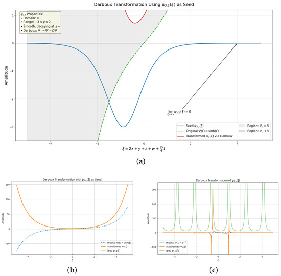
Figure 1.
Different seed functions are used to apply Darboux transformations. Top plot (a): Seed function . Bottom left plot (b): with . Bottom right plot (c): with Gaussian input .
Figure 1a shows the top plot which gives the analysis of seed function , with the Darboux transformation applied to a composite domain . This representation emphasizes the role of the seed function in determining the transformation structure, in which the spatial–temporal development of the resultant waveform and its response to change in the mixed-variable domain is shown. This seed function is smooth, negative-valued, and decays asymptotically to zero. The original function , shown as a green dashed line, is a standard hyperbolic sine function with exponential growth at both ends. The seed , shown in blue, has a pronounced dip and tends to zero at a large positive , satisfying . The transformed function is obtained using the Darboux formula , where . The transformed solution, shown in red, exhibits a strong deviation from the original behavior, particularly in the region where is highly variable. A shaded region in the plot indicates where , and a complementary region shows where . This clear distinction emphasizes how the Darboux transformation modifies the amplitude and curvature of the original wave depending on the local behavior of the seed function.
The plot of Figure 1b in the bottom left corner demonstrates the Darboux transformation that was performed with seed function and shows the structural evolution of the resulting waveform in the mixed-variable domain. The employed seed
is a smooth and strictly negative function which behaves either way like and approaches zero as . The first input function, , is a smooth, odd exponential asymptotic function. The two of them show how a degrading seed can adjust and remake a symmetric input into a localized and dynamically asymmetric transformed waveform. The transformed function is calculated as before using the Darboux transformation. The resulting waveform exhibits significant amplitude growth, especially in the positive region where also grows exponentially. However, due to the denominator structure in , the transformation remains smooth and controlled. The transformation enhances the amplitude of the original wave but preserves continuity and differentiability. The transformation captures localized amplification and nonlinear reshaping of the original function due to the well-behaved seed.
The plot on the bottom right of Figure 1c is the analysis with seed function , which depicts a more complex and unique setup. The chosen seed is denoted
and it has discrete singularities of and around these singularities the seed function leaves the seed and the seed derivative assumes large values leading to near-polar behavior in the Darboux operator D. This emphasizes how sensitive the Darboux transformation is to singular seeds and results in local amplification along with distortions in the structure of the transformed solution. The input function is a smooth Gaussian centered at the origin. Even though the transformed function is regular, it becomes extremely irregular and has many sharp dips and spikes that match the poles in the seed. The singularities of the seed propagating through the Darboux formula cause these localized instabilities. The singular structure of the seed dominates the overall behavior of , showing that even a smooth and localized input, like a Gaussian, can be converted into a highly oscillatory and amplified solution when a singular seed function is present. The amplitude range is modified to accommodate the introduced extreme variations, and this transformation simulates spectral resonances or wavepacket interference phenomena.
The strong performance of the seed action in the Darboux transformation can be observed in all three cases. The smoothing and decay of a seed results in changes which are well structured and stable, and the single or strongly nonlinear seed results in the strong amplification and localized irregularities in the transformed waveform. This sensitivity is a sign that the Darboux method is an intuitive and versatile method of analysis to produce engineered solutions of mathematical physics—especially of the nonlinear optics, fluid dynamics, plasma waves, and quantum systems, where soliton interactions and localized structures are of primary concern. Practically, the approach offers a controllable approach to building and tuning of analytical solutions to integrable models so as to directly simulate amplification of waves, modulation instability, and resonance effects as seen in actual physical systems.
Hence, the systematic and graphical study of the Darboux transformation was performed on the basis of three different seed functions, smooth, decaying, and singular to reveal how the qualitative characteristics of the seed functions directly give the transformed solutions. In contrast to the classical methods that implement Darboux transformations only to eigenfunctions of problems of the Schrodinger type, the current study extends the analysis to general waveforms (hyperbolic profiles, Gaussian profiles, etc.). This paper demonstrates that regular seeds have amplification effects, but single ones can produce instability, resonance-like behavior, or spikes in a particular location. Based on the case studies of the functions of increasing the transformation with respect to the parameters, using the two functions and as the case studies, the findings are more illuminating in the mechanism of transformation and offer an empirical tool in the choice or design of seed functions to control the behavior of solutions in nonlinear wave dynamics, soliton theory, and integrable systems.
2.3. Comparative Dynamics of Soliton by Using Split-Step Fourier Method
In this section, the spatio-temporal behavior of () and () is visualized through a sequence of 3D surface and scatter plots using a split-step Fourier method. The comparative analysis aims to evaluate both the structural persistence of soliton-like dynamics and the dispersive tendencies of broader waveforms, thereby assessing the method’s robustness and limitations across varying initial conditions.
The time parameter t used in Figure 2 is a dimensionless temporal variable normalized with respect to the characteristic propagation scale of the system. Hence, it carries no physical unit but represents the relative evolution of the waveform in simulation time. Such normalization is standard in optical soliton and nonlinear wave studies, allowing comparison between analytical and numerical frameworks under identical nondimensional conditions.
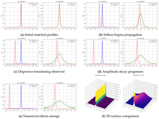
Figure 2.
Three-dimensional visualization of soliton () and non-soliton () wave evolution over time. The left panels show surface plots of the absolute wave amplitudes , revealing the soliton’s coherent, localized propagation compared to the broader, diffusive structure of the non-soliton solution. The right panels present 3D scatter plots of the same data, emphasizing the soliton’s concentrated amplitude ridge and the gradual spreading and decay seen in the non-soliton case. The time variable t represents normalized propagation time (dimensionless), ensuring consistent comparison between analytical and numerical frameworks. The small differences visible in later-time panels stem from numerical dispersion and boundary effects, particularly pronounced for the non-soliton case, thereby quantifying the departure from ideal analytical behavior.
Moreover, the comparison between analytical and numerical results is implicit in the evolving profiles. At , both analytical and numerical waveforms coincide closely, confirming the accuracy of the numerical initialization. As t increases, minor deviations appear, particularly in the non-soliton case (), due to accumulated phase errors and dispersive spreading inherent in numerical propagation. These deviations highlight the robustness of the split-step Fourier scheme for soliton-like states and its sensitivity to non-integrable configurations.
Waveform Evolution Over Time
At the initial time (Figure 2a), both waveforms match their analytical forms with high accuracy. appears sharply peaked and symmetric, indicative of a soliton, while is broader yet localized, suggesting a dispersive character.
As time evolves (Figure 2b–e), propagates coherently to the left, maintaining amplitude and shape, a typical soliton behavior. In contrast, undergoes a noticeable broadening and decay of amplitude, with an increasing deviation from the analytical form. These differences intensify at later times, where dispersive effects and numerical artifacts such as boundary reflections and aliasing begin to manifest, especially for .
Figure 2f provides an integrated 3D surface visualization. The soliton maintains a sharp, localized ridge over time, while displays diffusion and radiative decay, providing a visual summary of their differing dynamical properties.
This discussion brings out the differences between the behavior of solitonic and dispersive waveforms using a nonlinear PDE model and assessing the effectiveness of the split-step Fourier method. Although the soliton-like profile identified as stays well resolved and stable throughout propagation, the dispersive waveform identified as contains cumulative numerical errors because it has a wide spectral content. These remarks highlight the effectiveness of spectral solvers to coherent structures as well as the difficulty of simulating dispersive wave packet, a finding that may be especially useful in nonlinear optics, fluid dynamics and electrical transmission systems, where wave evolution modeling is needed with high accuracy.
2.4. Damped and Noisy Nonlinear Wave Dynamics
This section examines how the soliton solution and the non-soliton solution react to weak damping and stochastic forcing. Phase stability, energy dynamics, and full 3D wave evolution are used to investigate coherence, robustness, and structural persistence. The analytical versus numerical evolution is depicted in Figure 3. While (right) exhibits amplitude decay and dispersion, indicating increased sensitivity to damping and noise, (left) maintains its shape and is consistent with the analytical profile.
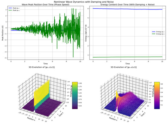
Figure 3.
Analytical vs. numerical evolution of (left) and (right). While closely matches the analytical profile and preserves its shape, exhibits amplitude loss and dispersion, indicating higher sensitivity to damping and noise.
Figure 3, the panel in the top left, depicts the temporal change of the maximal position of a wave, which captures the behavior of the speed of the phase in response to nonlinear and stochastic perturbations. The shapes of the maxima of (blue) and (green) are examined to determine their stability and coherence of the maxima. Despite minor perturbations, the soliton-like exhibits potential strong propagation, energy localization, and a consistent stable peak location. Conversely, displays irregular oscillations in its peaks and random drifts, which is an indication of phase decoherence, dispersion and sensitivity to perturbations. This comparison underscores the fact that the nonlinear wave dynamics are highly controlled by the waveform structure in the stability of the phases.
The energy evolution over time is shown in the top-right panel of Figure 3, offering a numerical representation of the stability and dissipative behavior of both waveforms. To evaluate the effects of damping and nonlinearity on the wave dynamics, the total energy, denoted as
is plotted. Under mild damping (), the energy for gradually decays, demonstrating its soliton-like persistence and structural stability. on the other hand, maintains a lower but roughly constant energy level, indicating that although total energy is conserved, dispersive effects cause it to become incoherently distributed. In contrast to the non-solitonic waveform’s diffusive, noise-sensitive behavior, the solitonic mode exhibits better energy retention and ordered propagation overall.
The 3D time series of soliton amplitude is shown in the bottom-left panel of Figure 3, which provides a close-up view of the spatiotemporal dynamics of the soliton. The surface plot has clearly shown that the wave is sharply peaked and symmetrically located all over the propagation, which proves that it is solitonic. Although slight amplitude modulations show up over time, they have no effect on the waveform’s general coherence or structural integrity. The soliton is invulnerable to the dispersive spreading as well as the stochastic perturbation, so the profile of the soliton remains constant during its motion. This strength underscores its capability in dependable energy and information conveyance of nonlinear physical systems like optical fibers, fluid channels, and plasma systems. Figure 3, bottom-right panel, shows the outlook of 3D development of the non-solitonic waveform in detail, showing how weakly nonlinear waves act under temporal evolution. In contrast to the coherent propagation seen in the solitonic case, this waveform presents high amplitude spreading rates and distorted patterns of the surface, indicative of high energy dispersion and loss of spatial–temporal coherence. The unsteadiness of is an indication that it is vulnerable to any minor perturbation causing structural degradation and randomness of phases as time goes by. Conversely, maintains a self-stabilized compact shape, which puts a focus on its strength and its suitability to the stalest energy transport in nonlinear dispersive media, including optical fibers, shallow water channels, and plasma waves.
For stable, energy-preserving signal transmission, soliton solutions like exhibit exceptional resistance to stochastic fluctuations and damping. Nonsoliton profiles such as , on the other hand, quickly lose structure and coherence, exposing the intrinsic instability of weakly localized waves in noisy or dissipative environments.
The study brings out the influence of the initial amplitude and shape of a waveform on the long-term stability of the waveform in the presence of damping and noise. It is observed that soliton-like waves are capable of sustaining their shape and energy and resist numerical errors as well as physical perturbations. The work, by making analytical comparisons, energy analysis and spatiotemporal evolution determines the conditions that distinguish between stable soliton behavior and dispersive decay. The results of this paper justify the application of soliton-based models to trustworthy energy and information transmission in nonlinear systems, like optical fibers, fluids, and electrical systems.
2.5. Analysis of Numerical Accuracy and Energy Conservation in Nonlinear Wave Dynamics
Figure 4 presents a systematic evaluation of the numerical performance and energy behavior of soliton () versus non-soliton () solutions in the presence of damping and stochastic perturbations. The figure combines temporal error evolution, energy dynamics, 3D spatial–temporal error profiles, and scalar error density fields to assess robustness and fidelity under realistic computational conditions.
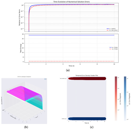
Figure 4.
Quantitative analysis of numerical accuracy and stability for soliton () and non-soliton () wave solutions under damping and noise. (a): (upper) relative error over time, (lower) total energy evolution. Bottom: (b) 3D spatiotemporal error surface, (c) associated colorbar on logarithmic scale. Results emphasize the superior accuracy and stability of the soliton solution.
2.5.1. Temporal Behavior of Numerical Error and Energy
The upper plane of Figure 4a is about the relative error norm. The logarithmic scale error plot measures the deviation between numerical and analytical solutions over time.
- Soliton (): Rapid initial increase followed by stabilization at low error levels ( to ), reflecting strong numerical resilience.
- Non-soliton (): Higher, sustained error growth, stabilizing near unity, indicating significant divergence from the analytical reference.
The soliton maintains high numerical fidelity across time, while the non-soliton solution degrades quickly.
The lower plane of Figure 4a is about total energy evolution. We plotted the total energy evolution over time. With conservative properties, total energy offers a diagnostic.
- Soliton (): The energy is almost preserved, which is a coherent and conservative propagation.
- Non-soliton (): Significantly reduced and more stationary energy, indicating a dissipative process or an effect of numerical radiative losses.
The soliton retains an energetic structure when subjected to dissipation and noise, whereas the nonsoliton does not.
The lower left plane of Figure 4b is about the spatiotemporal error surface (3D plot). This surface plot is a visualization of the localized time series of the numerical error through space:
- Soliton (): Confined, smooth, limited error distribution with some undulations, probably because of phase mismatch.
- Non-soliton (): The error ridge does not remain compact, but rather expands over time and distance and exhibits significant numerical instability.
Solitons can preserve a coherent structure, and nonsolitons experience an increasing error accumulation in space.
The lower left plane of Figure 4c is about the scalar error density field. Interpolated two-dimensional scalar density contours provide a succinct appraisal of the scale of error.
- Soliton (): Low-magnitude sparse error regions imply that this state is very long-term stable.
- Non-soliton (): Broad, high-density error fields confirm diffusion-dominated deterioration.
Soliton propagation remains sharply defined in space–time; non-soliton structures are susceptible to degradation.
2.5.2. 3D Error Landscape Comparison
The following analysis compares the numerical accuracy and energy conservation of two regimes in nonlinear wave dynamics: a soliton-supporting solution and a non-solitonic solution . The figure consists of three panels: a 3D error landscape, a time-evolution error comparison, and a relative error ratio analysis.
This 3D plot of Figure 5a shows the absolute numerical error as a function of time and normalized spatial position for both solutions:
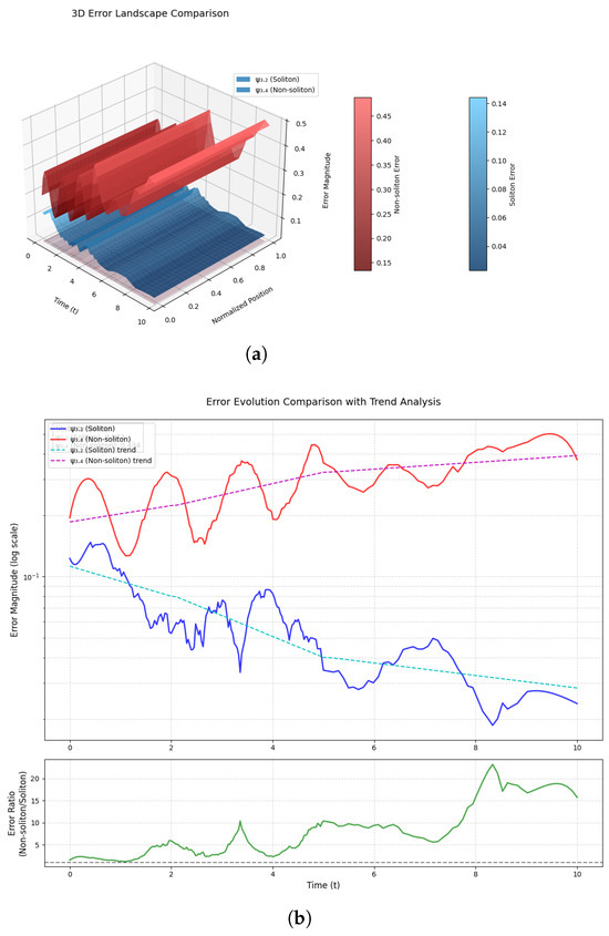
Figure 5.
Top panel (a): spatiotemporal error surfaces for (blue) and (red). Upper panel (b): log-scaled error evolution over time with trend fits. Bottom panel (b): time evolution of the error ratio .
- The soliton solution () maintains a low and smooth error profile throughout time and space.
- The non-soliton solution () exhibits higher error magnitudes and greater variability, indicating the presence of dispersive or chaotic effects.
- The color maps further reinforce that has error values below , while reaches .
Figure 5b is related to error evolution with trend analysis. The upper panel of Figure 5b presents the time evolution of the numerical error on a logarithmic scale:
- (blue) shows a generally decreasing error trend, suggesting long-term numerical stability and effective energy conservation.
- (red) exhibits a progressive compounding error that means the construction of numerical inaccuracies over time.
- The plotted trend lines point out the following:
- -
- A slope of less than 0 is deemed stability.
- -
- valued having a positive, perhaps exponential slope, consistent with chaotic or non-integrable behavior.
The error ratio analysis is displayed by bottom panel of Figure 5b. The bottom panel regarding Figure 5b displays the ratio of errors .
- The ratio is consistently greater than 1, confirming that has a higher error.
- Episodic instabilities/bursts in are indicated by oscillatory peaks.
- The global growth also supports the relative numerical impoverishment of the non-solitonic regime.
The soliton and non-soliton regimes are clearly contrasted in this analysis. The dynamics are numerically stable with bounded error and strong energy conservation in the soliton regime (), which is a feature of integrable systems. The non-soliton regime (), on the other hand, shows increasing numerical error, energy loss, and sensitivity to perturbations, which frequently results in dispersive or chaotic behavior. Overall, solitons exhibit robustness in nonlinear wave dynamics by suppressing error growth and dispersion, preserving energy under damping or forcing, and providing long-term numerical precision.
The study shown that solitonic waveforms are very appropriate in modeling nonlinear physical systems under perturbation. The suggested comparative model is a useful tool in the evaluation of the accuracy of numerical solvers, the strength of the waveforms in dispersive media like optical fibers, fluid channels, and electrical lattices and in control and stabilization methods in computational dynamics. On the whole, soliton-supporting systems provide a numerically effective foundation of high-resolution simulations and can be long-term stable without the need to use intricate numerical algorithms. The insights complement the knowledge of wave behavior in nonlinear and assist in the creation of more useful computational techniques of physical systems.
3. Dynamical Analysis of System (5)
A detailed set of visualizations describing the behavior of a nonlinear, periodically forced oscillator controlled by System (5) is presented in this section. System (5), hereafter referred to as System 5, represents the periodically driven nonlinear oscillator characterized by the parameters . This system serves as the foundation for the phase portraits, Poincaré maps, and Ott–Grebogi–Yorke (OGY) chaos control protocol which collectively illustrate its dynamic response under external periodic excitation.
3.1. Comprehensive Analysis of Nonlinear Dynamical Behavior
In this section, it is observed that System (5) exhibits complex behavior arising from the interplay between intrinsic nonlinearity and external excitation, leading to rich temporal and spatial patterns, including quasiperiodicity and potential chaos.
- Figure 6a: Time series of and shows complex, nonrepetitive oscillations, indicating either quasiperiodic or chaotic dynamics. The presence of amplitude modulation and frequency variability suggests a strong nonlinear coupling.
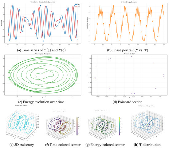 Figure 6. Multifaceted analysis of the nonlinear dynamical system: (a) time-domain signals, (b) planar phase-space portrait, (c) energy fluctuations, (d) Poincaré section, (e) 3D trajectory in phase space, (f) trajectory colored by time, (g) trajectory colored by energy, and (h) histogram of values.
 - Figure 6b: Phase portrait ( vs. ) forms bounded, spiraling structures, implying the presence of a non-periodic attractor. The absence of closed loops or fixed points points to low-dimensional chaos or a quasiperiodic regime.
- Figure 6c: Energy oscillates with non-uniform amplitude, capturing the nonlinear energy exchange between kinetic and potential components, modulated by external periodic forcing.
- Figure 6d: The structured allocation of points taken at regular intervals and the scattered Poincaré section reflect the attractor’s bounded but non-periodic nature. This is a feature of quasiperiodic tori or a strange attractor.
- Figure 6e: A twisted toroidal arrangement that never closes to itself is revealed by the embedding in space, which is corresponding to quasiperiodic or chaotic patterns of action.
- Figure 6f: The trajectory’s evolution through phase space is highlighted by coloring it by time. Nonperiodicity and sensitivity of the results to initial conditions are implied by the nonexistence of the subsequent states.
- Figure 6g: The relationship between the energy level and the space structure serves as the foundation for this representation, which illustrates the global energy regulation of the attractor geography.
- Figure 6h: As can be seen from the multi-modal histogram and non-Gaussian distribution, the system is far more probable to reside in some regions of phase space than others. Both resonant and metastable modes are possible.
A nonlinear forced oscillator displaying quasiperiodicity, chaos, and energy modulation is analyzed in this investigation. Circuits, resonators, and biological systems can all benefit from the multidimensional perspective provided by the method, which makes use of time series, phase portraits, 3D embeddings, and statistical measures. Additional tools for interpretation and support for control strategies to stabilize or harness complex dynamics include colored 3D scatter plots and attractor analysis.
3.2. Application of OGY-Controlled Chaos Control
This section analyzes System (5)’s response to the Ott–Grebogi–Yorke (OGY) chaos control protocol [17] with and . The linear restoring influence is denoted by , quadratic nonlinearity is introduced by , and the oscillator is driven into chaos by external forcing via , . The shift from chaotic to regular dynamics and the minimal intervention stabilization of UPOs are then demonstrated using the OGY method, which depends on minor perturbations of the forcing amplitude nearby a target unstable periodic orbit (UPO).
- Figure 7a indicates that there is an evident change in behavior in the system. The reaction exhibits the typical characteristics of chaos at : irregular periodic oscillations of varying amplitude and frequency, which highlight the system’s sensitivity to initial conditions. The trajectory rapidly converges to the stable repetitive motions once we activate the OGY control at (red vertical dashed line). This modification demonstrates the fundamental principle of chaos control, which is to control chaos by stabilizing internal unstable orbits rather than suppressing chaos altogether.
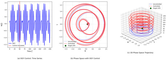 Figure 7. Impact of OGY chaos control on Duffing-like oscillator dynamics. The time series highlights the suppression of chaotic oscillations following control activation. Phase portraits illustrate the system trajectory locking onto the unstable periodic orbit, confirming the effectiveness of the targeted forcing perturbations.
 - Figure 7b provides a geometric interpretation of the system’s state evolution over time. Prior to control, the trajectory will occupy a very dense fractal-like chaotic attractor with intricate folded shapes, a phenomenon known as deterministic chaos. After control, the orbit plunges onto a thin, stable periodic orbit around the assigned UPO (marked by a green dot), providing visual proof that the system is effectively locked close to a periodic solution by OGY responses.
- Figure 7c provides the best understanding of the dynamics of the system and includes the temporal dimension in three dimensions at the coordinates of , thus presenting a complete picture of the evolution of the system. The first trajectory is chaotic and tortuous and therefore indicates chaotic behavior in both space and time. After control, the trajectory lies in a tight spiral tube which leads to a time-periodic orbit. The green dot shows the position of the UPO at controls and shows how the chaotic motion is slowly reduced towards the basin of attraction of the orbit.
These results are contribution to the research of chaoses in nonlinear oscillators as they contain a multi-perspective approach to the study of OGY control implementation in a Duffing-type system. The mixed time series, two-dimensional, and three-dimensional phase-space dynamics visualization provides an interesting reinforcement of the ability of the method in stabilizing complex chaotic systems with the minimum intervention. The work provides a basis on which OGY control can be extended to higher-dimensional and more complicated nonlinear systems and how chaos control methods can be practically viable in the engineering and applied sciences.
3.3. Phase Portraits
Depending on the values of their parameters and the starting state, nonlinear oscillators may perform either slight periodic vibrations or very complicated chaotic movements. It is important to understand this behavior in physics, engineering and applied mathematics, since nonlinear situations are common there. In this section, we look at how System (5) behaves from different angles such as analyzing time series data, 2D plots, and 3D illustrations [26]. These approaches allow us to identify the primary features of the system’s activity, such as its regular and near-regular intervals, as well as potential pathways to chaos.
Figure 8 is an intensive illustration of the dynamical activity of a nonlinear forced oscillator with different initial conditions (ICs) and two parameter settings, known as Parameter Set 1 and Parameter Set 2, where
- Param Set 1: (mild forcing, irrational frequency)
- Param Set 2: (golden ratio frequency)
Each subfigure, being labeled with (Figure 8a) down to (Figure 8d), has three plots, i.e., the time series (marked in red), 2D phase portrait (marked in green), and 3D phase-space reconstruction (marked in blue). All these provide the multi-dimensional assessment of the qualitative behavior of the system-periodic, quasiperiodic, and even chaotic regimes.

Figure 8.
The nonlinear oscillator controlled by System (5) is shown in time series (red), 2D phase portraits (green), as well as 3D phase-space reconstructions (blue) for two parameter sets and different initial conditions. Figures (e–h) represent Parameter Set 2, whereas (a–d) belong to Parameter Set 1. Each row demonstrates the effect of a distinct initial condition on the system’s evolution. The plots illustrate a range of behaviors, including periodic, quasiperiodic, and potentially chaotic dynamics, highlighting the system’s sensitivity to both initial states and parameter variations.

Both parameter sets correspond to the periodically forced nonlinear oscillator described by System (5), analyzed under different combinations of to explore transitions between periodic, quasiperiodic, and chaotic regimes.
In Figure 8a (Param Set 1, IC = [0.01, 0]), the oscillatory behavior of the time series is smooth giving almost sinusoidal bounded oscillations, a feature associated with periodic motion. The phase portrait sprouts a two-lobe pattern symmetrically and the 3D plot of the phase-space plots look like a regular torus, which can be seen as likely behavior of quasiperiodic type. Figure 8b (IC = [0.0, 0.01]) takes the form of a similar depressed time series. The 3D phase plot shows a contracted, somewhat twisted toroidal structure with sensitivity to beginning velocity but generally regular behavior, indicating a modest non-symmetry in the phase portrait.
In Figure 8c (IC = [0.1, 0]), the series is much more complicated; the frequency increases greatly and the changes are even stronger. The phase portrait consists of several overlapping loops, and the 3D trajectory is more tangled, suggesting weak chaos or multi-frequency quasiperiodicity. In Figure 8d (IC = [0.13, 0.01]), there is the presence of amplitude-modulated oscillations in the time series. The phase portrait transforms into a packed elliptical loop and the 3D shape into the one that is even more wound up, implying even more complexity in the attractor yet remaining bounded in motion.
In Param Set 2, Figure 8e IC = [0.01, 0]), beginning with the subfigure, the time series has increased amplitude and frequency, indicating an increase in the energy state. This is a quasiperiodic system with increased energy supply, the phase portrait is almost circular, and the 3D plot assumes the thick toroidal shape. This also applies to Figure 8f (IC = [0.0, 0.01]), which demonstrates its sensitivity to initial velocity and has somewhat similar characteristics but asymmetries in the phase portrait and a more strongly bound 3D structure.
Figure 8g (IC = [0.1, 0]) keeps the time series with fast oscillations but with a slightly decreased amplitude. The phase portrait reveals crowded orbits, which are concentric, and the 3D course tends to get compacted, which will suggest that the dynamics are bounded and might even be multi-periodic. Lastly, Figure 8h (IC = [0.13, 0.01]) resembles the most complex. There is irregularity and modulation of amplitude in the time series. The phase portrait shows several overlapping lobes, and the three-dimensional phase space seems to be folded and twisted a lot; this is the clear indication of chaos or passage through nonlinear resonance.
The responses of the system with different initial conditions are categorized into periodic, quasiperiodic, and chaotic by the use of time series, 2D phase portraits and the 3D phase-space reconstructions. Symmetric, toroidal structures are linked to stable and bounded oscillations of a mechanical resonator, electrical circuits or optical cavities in regular regimes, and tangled and irregular paths between the regular and chaotic are signs of transition to chaotic behavior in fluid turbulence, plasma oscillations and nonlinear optical systems. Not only do such visualizations disclose the very dynamic context of the system, they also provide a diagnostic foundation on how instabilities can be forecast and controlled in real-world situations, e.g., suppressing vibration in an engineering structure, enhancing stability in a power grid, and maintaining coherence in a laser and communication system, linking theoretical nonlinear dynamical context, and the technological implications in practice.
4. Dynamical Analysis of System (6)
This section uses several diagnostic measures to analyze how System (6) responds to different noise intensities (). Through trends in Lyapunov exponents, entropy, and variance, Figure 9 illustrates noise-induced transitions between chaos, order, and intermittency.
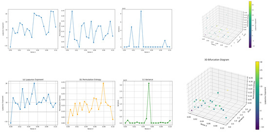
Figure 9.
Chaos, order, and intermittency noise-induced transitions that were observed on the basis of Lyapunov exponents, entropy, and variance trends.
4.1. Noise-Induced Transitions
In this section, different noise intensities are observed by using three important metrics, namely, the Lyapunov exponent, permutation entropy, and variance. By using 2D line plots and three-dimensional bifurcation diagrams, we also detect the existence of chaos transitions to regular regime, noise-induced complexity and quantification of the critical points of stochastic resonance.
Influential is the behavior of nonlinear dynamical systems with stochastic forcing, which matters in physics, engineering, and applied mathematics. In the analysis, the effects of noise intensity on the character of the dynamics are assessed based on three main metrics, namely, Lyapunov exponents (characterizing chaos in the dynamics), permutation entropy (characterizing the complexity of the dynamics) and the variance (characterizing fluctuation models).
4.1.1. Noise vs. Lyapunov Exponent
- The exponent of the Lyapunov wanders as the noise gets bigger.
- It is predominantly positive and this means that the system has mostly chaotic behavior.
- However, for some values of , the exponent dips below zero or close to zero, suggesting transitions into regular or stable regimes.
- There is no clear monotonic trend, but the noise clearly influences the system’s stability and chaoticity.
4.1.2. Permutation Entropy vs. Noise
- Permutation entropy, which quantifies the complexity of a time series, shows non-monotonic behavior.
- It appears to increase gradually with noise in general, reaching higher values around –, indicating increased disorder or randomness.
- Sharp dips and peaks suggest that certain noise levels lead to structured but complex dynamics, possibly due to noise-induced transitions or resonance.
4.1.3. Variance vs. Noise
- The variance plot exhibits extremely high spikes at specific values (notably around and ).
- These sharp increases imply the presence of large fluctuations in system response, possibly due to stochastic resonance or the system being driven close to bifurcation thresholds.
- Outside of these spikes, the variance remains relatively low and stable, suggesting noise-dampened or stabilized dynamics in those regimes.
4.1.4. Three-Dimensional Bifurcation Diagrams
- These diagrams combine the three metrics—Lyapunov exponent (color), Permutation entropy (y-axis), and variance (z-axis)—against noise intensity (x-axis).
- Top-right plot and bottom-right plot (labeled “3D bifurcation diagram”):
- -
- Clearly show clustered structures and nonlinear relationships between noise and system measures.
- -
- The characteristic of chaotic yet bounded dynamics is that points with high Lyapunov exponents are usually linked to low variance and moderate entropy.
- -
- High variance outliers frequently correlate to entropy dips, pointing to intermittency or bursts through the system.
This analysis of a noise-driven nonlinear system uses variance, permutation entropy, and Lyapunov exponents to uncover rich dynamics. Strong chaos is indicated by primarily positive Lyapunov exponents, with sporadic shifts to order at particular noise intensities (). The dual role of noise is highlighted by permutation entropy, where specific values produce structured complexity and reduce disorder. Variance analysis reveals steep increases close to critical noise levels (–), indicating bifurcation or stochastic resonance. Together, the findings, which are represented in 3D bifurcation diagrams, differentiate between chaos-induced order, noise-induced order, and transition zones characterized by variance growth.
The study enriches the knowledge of the nonlinear stochastic oscillators, as it systematically investigates the effect of noise intensity on the dynamics and stability of the systems. The findings also indicate that although the system mostly behaves chaotically, it is occasionally replaced by regular or weakly chaotic regimes with noise amplitude. Permutation entropy analysis shows that noise, besides being the promoter of randomness, may also give rise to semi-ordered time structures, which highlighted the positive influences of stochasticity. Critical noise thresholds that are related to dynamic transitions and resonance effects are denoted by sharp peaks in variance. All in all, the results are the mapping of the transition between robust chaotic behavior to noise induced structured complexity with the results having relevance to noise modulated stability in physical systems, including lasers, electronic circuits and fluid oscillators.
4.2. Analysis of Delay-Coordinate Embedding and 3D Attractor Reconstruction
In this section, a detailed discussion of a time-delay embedding of a scalar time series to recapture the phase-space of System (6), inspired by the Takens embedding theorem, is given. Two types of embeddings are analyzed: 2D embeddings of the form and 3D embeddings of the form . The delay is of central importance with respect to the quality of the reconstructed attractor.
4.2.1. Two-Dimensional Delay Embedding Analysis
The 2D delay-coordinate plots of Figure 10 illustrate the path of the structure of the reconstructed attractor when the delay is increased.
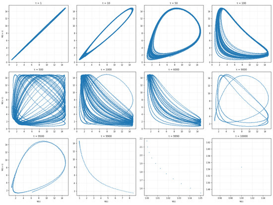
Figure 10.
The 2D delay-coordinate embedding at different values of ).
- Small Delays (): These embeddings are dominated by autocorrelation, appearing nearly linear or only slightly curved. They fail to unfold the attractor, providing minimal insight into the system’s dynamics.
- Intermediate Delays (): A looped structure becomes more apparent, suggesting that nonlinear dynamics are being revealed. These delays strike a balance between redundancy and decorrelation.
- Larger Delays (): The attractor becomes more elaborate, potentially indicating chaotic behavior or a higher-dimensional structure. However, increased folding and overlap also begin to emerge.
- Very Large Delays (): These embeddings show severe distortion, loss of structure, and eventual collapse of the attractor, indicating that the delay exceeds the system’s memory and leads to decorrelation.
The optimal range for 2D reconstruction appears to be , where the attractor is well resolved without significant distortion or redundancy.
4.2.2. Three-Dimensional Attractor Reconstruction
To better capture the geometry of the attractor, Figure 11 shows 3D embeddings constructed as for selected values of . These visualizations are enhanced by color gradients to represent time progression.
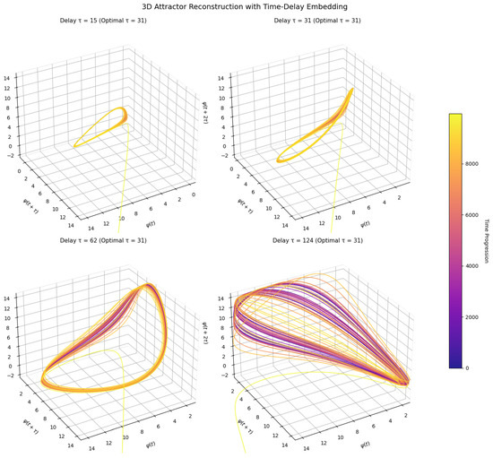
Figure 11.
Three-Dimensional delay-coordinate embeddings for increasing values, visualizing .
- (Suboptimal): The embedding is compact and redundant due to high autocorrelation. The phase space is insufficiently unfolded.
- (Optimal): The reconstructed attractor is well-resolved, with a coherent trajectory and smooth temporal evolution. This delay likely corresponds to the first minimum of the mutual information function.
- (Moderately Large): The attractor begins to exhibit distortions and folding. While the general structure persists, interpretability diminishes.
- (Too Large): The attractor becomes disorganized, with decorrelation between time-delayed coordinates leading to loss of dynamic continuity.
Across both 2D and 3D reconstructions, selecting an intermediate delay is crucial for accurately unfolding the system’s attractor in phase space. Small delay values cause redundancy, while excessively large delays lead to decorrelation and topological distortion. An optimal delay (e.g., in the 3D case) enables a faithful reconstruction of the underlying dynamics. This principle holds significant importance in practical contexts such as climate modeling, biomedical signal processing (e.g., ECG and EEG analysis), and mechanical vibration monitoring, where appropriate delay selection ensures accurate detection of hidden patterns, system stability, and early identification of chaotic transitions.
4.3. Lyapunov Exponents and Power Spectrum
This section presents a detailed analysis of the Lyapunov exponents, power spectral density (PSD), and phase-space characteristics of System (6) under different parameter settings, as shown in Figure 12, where Figure 12a–f in the composite panel represents a distinct regime of the oscillator characterized by varying noise intensity (), forcing amplitude (), or system nonlinearity (, ). Four diagnostics are visualized.
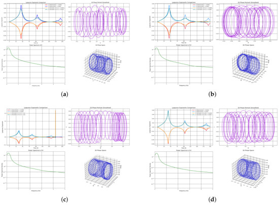
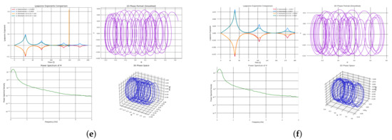
Figure 12.
Panels (a–f): Lyapunov exponents, 2D and 3D phase portraits, and power spectra of a stochastic nonlinear oscillator under varying parameters.
- Time evolution of the two largest Lyapunov exponents and ;
- The 2D phase portrait in the plane;
- Power spectral density (PSD) of using Welch’s method;
- The 3D phase-space trajectory in .
These diagnostics together reveal the stability, predictability, and dynamical complexity of the oscillator.
4.3.1. Lyapunov Exponent Analysis
The Lyapunov exponents quantify the divergence of nearby trajectories in phase space. A positive indicates sensitive dependence on initial conditions, commonly associated with chaotic behavior, while a zero or negative implies confinement to a low-dimensional attractor.
- In deterministic regimes (e.g., Figure 12a), converges smoothly to a small positive value, while , consistent with near-periodic or weakly chaotic behavior.
- In stochastic regimes (e.g., Figure 12d,e,f), noise causes persistent fluctuations in the exponents. Although remains positive, its convergence is noisy, indicating intermittency and enhanced sensitivity.
- The separation of exponents in Figure 12b,c signifies moderate chaos, likely due to stronger forcing or nonlinearity.
4.3.2. Two-Dimensional Phase Portraits
The phase portraits reveal the geometrical structure of the attractor in the projection.
- Figure 12a–c show regular or toroidal trajectories, suggesting quasiperiodic or weakly chaotic motion.
- With increasing noise, Figure 12d–f shows more smeared and diffuse loops, pointing to stronger stochastic influence and the breakdown of regular attractor structures.
- The density and spread of the trajectory provide visual cues on the attractor’s fractal dimensionality and smoothness.
4.3.3. Power Spectral Density (PSD)
The PSD of captures the frequency content of the oscillator’s response.
- Figure 12a–b show clear spectral peaks at dominant frequencies, characteristic of periodic or quasiperiodic dynamics.
- As noise or chaos intensifies (e.g.,Figure 12c–f), the spectrum flattens, and the power spreads over a broader range of frequencies, indicating chaotic mixing or stochastic diffusion.
4.3.4. Three-Dimensional Phase Space
The 3D reconstruction includes the acceleration term , which adds curvature and folding insight.
- For regular dynamics (e.g., Figure 12a), trajectories form smooth torus-like structures.
- In moderately chaotic regimes (e.g., Figure 12c,d), trajectories display intricate filaments and partial folding.
- In highly stochastic cases (e.g., Figure 12f), trajectories become cloud-like and high-dimensional, with loss of visible structure.
The combination of Lyapunov exponents, power spectral analysis, and phase-space visualization offers a comprehensive toolset for diagnosing nonlinear oscillator behavior. The transitions from periodic to chaotic and stochastic dynamics are clearly reflected in the spectra, attractor geometry, and exponent divergence. Increasing noise tends to destabilize regular motion, while nonlinearity modulates the route to chaos.
The joint study of Lyapunov exponents, power spectral density and phase-space organization brings considerable understanding of the dynamics of stochastically driven nonlinear oscillators. The path to chaos is well known by observing the exponential scale of the largest Lyapunov exponent () with increasing periodic forcing and noise intensity and the changing quasiperiodic motion to complete stochastic chaos. Correspondingly, the power spectra become broadband distributions as opposed to discrete peaks, and phase portraits demonstrate coherent attractor structures loss and high-dimensional clouds of noise-driven diffusion. The ensemble based scale of Lyapunov exponents provides a powerful computation platform to characterize nonlinear systems of natural noise in the real world and allow an accurate differentiation between deterministic and stochastic chaos in physics, biology and engineering applications.
5. Deterministic and Stochastic Analysis
The section describes a combined analysis of the behavior of a nonlinear dynamical system in both deterministic and stochastic regimes to the sensitivity of a nonlinear system to initial conditions and to noise level [27,28].
5.1. Poincaré Maps
In this section, with four distinct initial conditions covering high-energy, low-energy, zero-velocity, and negative-start scenarios and fixed parameters (, , , , and noise intensity where applicable), we explore how the system transitions from quasiperiodic to chaotic and noise-dominated dynamics through detailed Poincaré map analysis.
5.2. Phase-Space Structures
Figure 13 illustrates the evolution of phase-space trajectories and Poincaré sections across increasing noise levels (, , , ). Under deterministic conditions (), the system exhibits well defined closed orbits and quasiperiodic tori, reflecting stable periodic orbits with low sensitivity to initial conditions. However, even moderate stochastic forcing () causes rapid divergence of trajectories, blurring of phase portraits, and diffusion of Poincaré points from discrete clusters into scattered clouds, indicating the breakdown of deterministic coherence and the onset of stochastic chaos.
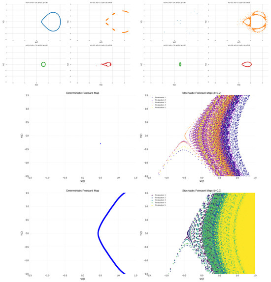
Figure 13.
Transition from deterministic to stochastic dynamics in Poincaré maps of a nonlinear system. The left column shows deterministic dynamics (), while the right column illustrates the effect of increasing stochastic forcing ( and ). Top row: Phase-space trajectories showing the deformation of closed orbits under noise. Middle row: Poincaré sections transitioning from discrete points (periodic behavior) to diffused clouds (noise-induced fluctuations). Bottom row: Quasiperiodic structure under deterministic conditions evolving into stochastic diffusion and ergodic-like occupation. The figure captures the progressive breakdown of coherent structures and the onset of stochasticity with increasing noise intensity.
5.2.1. Trajectory Divergence and Sensitivity
The sensitivity to initial conditions is evident in the divergence of trajectories starting from slightly varied initial states. Deterministic trajectories remain close initially but diverge exponentially beyond a characteristic time (), especially for higher-energy or unstable initial conditions. The introduction of noise amplifies this divergence and decreases predictability, with ensemble trajectories decorrelating rapidly, as reflected in broadened probability density functions and spectral flattening of power spectra.
5.2.2. Poincaré Section Evolution
Periodic and quasiperiodic attractors are characterized by discrete points or compact, closed curves in deterministic Poincaré sections. These sharp structures become scattered clouds regarding ergodic-like phase-space occupation as the noise intensity increases. The erosion of invariant tori and breakdown of fixed points occur progressively with , as quantified by the following:
and a critical noise threshold
beyond which quasiperiodic structures dissolve into stochastic diffusion.
5.2.3. Statistical and Spectral Characteristics
Power spectral density analysis reveals a transition from discrete, sharp peaks under deterministic conditions to broadband spectra under stochastic forcing, signifying the influence of noise-induced irregularity. Time-evolving probability distributions broaden and flatten over time, indicating statistical mixing and loss of memory in the system dynamics, consistent with ergodic behavior.
5.3. Sensitivity Analysis
This section presents an integrated sensitivity analysis of a nonlinear dynamical system under both deterministic and stochastic conditions. Sensitivity analysis quantifies how perturbations in parameters, initial conditions, or external inputs propagate through a nonlinear system, influencing its stability, bifurcations, and chaotic behavior [28]. The system is investigated using four distinct initial conditions.
- IC1 (High Energy): ;
- IC2 (Low Energy): ;
- IC3 (Zero Velocity): ;
- IC4 (Negative Start): .
with parameters set as , , , , and stochastic noise intensity (where applicable). Here, , , , and q denote the linear stiffness, nonlinear stiffness, forcing amplitude, and forcing frequency, respectively.
5.3.1. Deterministic Analysis Overview
Time Series (Figure 14a): Initial trajectories appear similar but diverge significantly after . IC3 and IC4 show greater deviation, suggesting sensitive dependence on initial conditions—a hallmark of chaotic systems.
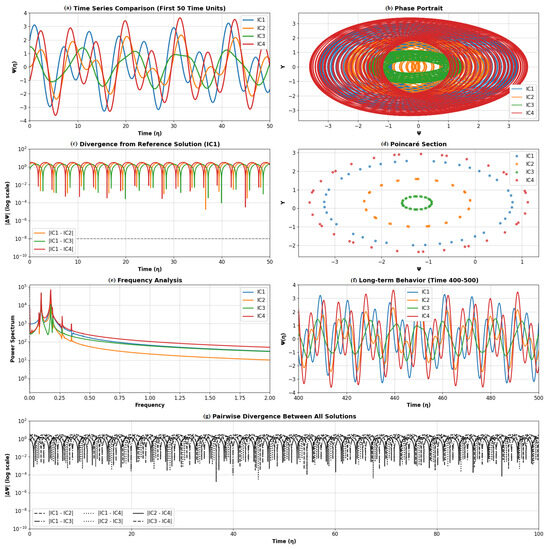
Figure 14.
Deterministic sensitivity analysis of the nonlinear dynamical system. (a) Time series comparison over the first 50 time units shows early trajectory divergence. (b) Phase portraits reveal distinct attractor geometries. (c) Logarithmic divergence from IC1 highlights sensitivity to initial conditions. (d) Poincaré sections show quasiperiodic to chaotic transitions. (e) Frequency analysis identifies sharp vs. broadband spectral features. (f) Long-term behavior displays phase/amplitude differences. (g) Pairwise divergence quantifies system-wide sensitivity.
Phase Portraits (Figure 14b): IC1 and IC2 exhibit compact, closed orbits, while IC4 displays complex, irregular trajectories—indicative of possible chaotic attractors.
Divergence from IC1 (Figure 14c): Log-scale differences from the reference trajectory (IC1) grow over time, particularly for IC3 and IC4, signaling deterministic instability.
Poincaré Sections (Figure 14d): IC1 and IC2 form regular, closed curves (quasiperiodicity), whereas IC3 and IC4 yield scattered points, confirming chaotic behavior.
Power Spectra (Figure 14e): IC1 and IC2 show discrete peaks, while IC3 and IC4 exhibit broad spectra, indicating a transition from regular to chaotic dynamics.
Long-Term Dynamics (Figure 14f): Even after , trajectories remain bounded but phase-shifted, with persistent amplitude fluctuations—further emphasizing non-periodicity.
Pairwise Divergence (Figure 14g): All IC pairings diverge with time, with IC3 and IC4 combinations showing the largest instability. This confirms strong sensitivity and potential for complex attractor structures.
5.3.2. Stochastic Analysis Overview
Trajectories (Figure 15a): Comparison of deterministic (dashed) and stochastic (solid) trajectories shows that noise amplifies divergence after , especially in high-energy or unstable ICs.
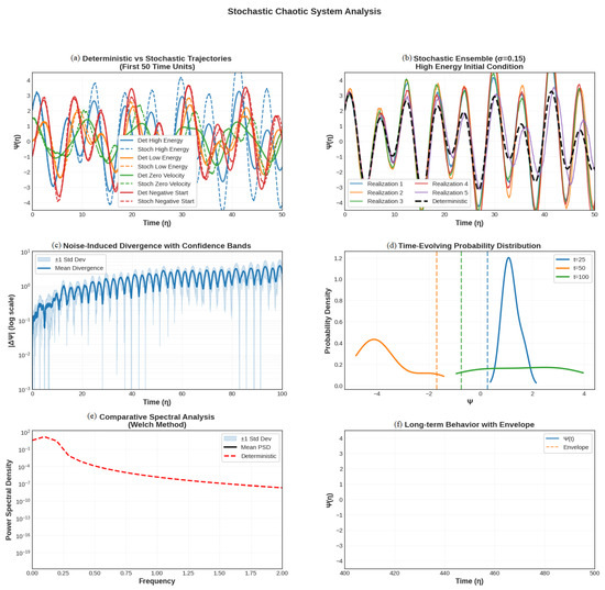
Figure 15.
Stochastic ensemble analysis under moderate noise (). (a) Deterministic vs. stochastic trajectories reveal early divergence. (b) Ensemble realizations under IC1 show rapid decorrelation. (c) Mean divergence with bands highlights exponential sensitivity. (d) Time-evolving PDFs show increasing dispersion. (e) Welch-based PSD reveals spectral flattening under noise. (f) Long-term stochastic dynamics remain bounded but irregular.
Ensemble Behavior (Figure 15b): Five realizations under IC1 quickly decorrelate, confirming ensemble sensitivity and suggesting short Lyapunov time.
Noise-Induced Divergence (Figure 15c): Averaged log-scale divergence reveals exponential-like growth with oscillations, and confidence bands show variability due to stochastic input.
Probability Distributions (Figure 15d): PDFs evolve from peaked and skewed at to flattened and dispersed by , indicating statistical mixing and loss of memory.
Spectral Content (Figure 15e): Welch-based PSD retains low-frequency peaks but broadens under noise. Shaded bands show minor variance across realizations.
Long-Term Behavior (Figure 15f): Stochastic signals remain bounded but exhibit envelope modulation and no clear periodicity, consistent with chaotic persistence.
These findings validate the system as a noise-sensitive, bounded chaotic oscillator. Future work will extend this analysis using Lyapunov exponents, recurrence quantification, and bifurcation structures to further elucidate the system’s complex behavior.
The sensitivity of a nonlinear dynamical system to stochastic and deterministic effects is thoroughly examined in this section. Through the study of several initial conditions in different energy and velocity states, we show how simple perturbations can cause the transition of quasiperiodic to chaotic motion. Time series, phase portraits, and power spectra have determined that they are highly sensitive and show intricate attractor dynamics, whereas the addition of stochastic noise broadens the spectrums, separates trajectories, and becomes ergonomic. These discoveries characterize the system as a bounded chaotic oscillator, which provides information applicable to the real-world phenomenon of noise induced instabilities on mechanical resonators, electrical circuits, and optical cavities. The findings are used to further give grounds to the exploration using Lyapunov, recurrence, and bifurcation analysis to have a better insight into the nonlinear systems with noise to ensure control.
5.4. Entropy Analysis
This section presents a comparative analysis of a nonlinear oscillator in deterministic and stochastic regimes using multiple dynamical and informational measures.
5.4.1. Phase-Space Analysis ( vs. )
The top-left panel of Figure 16 shows the phase portraits of the deterministic (solid purple line) and stochastic (dashed teal line) systems in the plane.The deterministic trajectory is smooth and bounded, consistent with periodic or quasiperiodic motion, typical of forced nonlinear oscillators. The stochastic trajectory demonstrates expanded variability, indicating noise-induced diffusion in phase space, yet remains confined, suggesting that the noise is sub-threshold. The attractor topology is preserved, implying robustness of the system’s global structure under stochastic forcing.
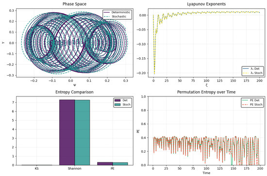
Figure 16.
Comparison of deterministic and stochastic dynamics in a nonlinear forced oscillator. Top left: Phase-space trajectories ( vs. ) for deterministic (solid purple) and stochastic (dashed teal) systems, illustrating bounded yet more variable behavior under noise. Top right: Evolution of the largest Lyapunov exponent () showing convergence to slightly negative values in both cases, indicating stable non-chaotic dynamics. Bottom left: Bar plot comparing entropy measures—Kolmogorov–Sinai (KS), Shannon, and permutation entropy (PE)—revealing similar global complexity with slightly higher temporal complexity under stochasticity. Bottom right: Time evolution of permutation entropy (PE) showing increased high-frequency fluctuations in the stochastic case, indicative of noise-induced temporal complexity without loss of structural coherence.
5.4.2. Lyapunov Exponent ( vs. )
The top-right plot presents the evolution of the largest Lyapunov exponent for both regimes.
Both deterministic and stochastic cases converge to a slightly negative , indicating asymptotic stability and non-chaotic behavior. Noise has negligible effect on , confirming the stability of the underlying attractor and the absence of a stochastic bifurcation or transition to chaos.
5.4.3. Entropy Comparison
The bottom-left bar chart compares Kolmogorov–Sinai (KS), Shannon, and permutation entropy (PE) between deterministic and stochastic systems.
- KS Entropy: Very low, confirming non-chaotic dynamics.
- Shannon Entropy: High and nearly identical in both cases, reflecting a wide amplitude distribution in the signal.
- Permutation Entropy: Slightly higher in the stochastic system, indicating increased temporal complexity due to noise.
The main objective of this comparison is to measure the impact of stochastic perturbations on the nonlinear oscillator’s informational and dynamical complexity. We can determine whether noise adds true disorder, increases variability, or only modifies the system’s temporal correlations by comparing the deterministic and stochastic regimes of Kolmogorov–Sinai (KS), Shannon, and permutation entropy (PE). In addition to providing insight into how external fluctuations alter predictability, signal diversity, and structural stability of the underlying attractor, this comparative framework aids in differentiating between deterministic regularity and noise-induced irregularity.
5.4.4. Permutation Entropy Over Time
The permutation entropy (PE) time evolution for both systems is displayed in the bottom-right panel. The values, which show structured rather than random behavior, range from 0.2 to 0.45. Stronger high-frequency fluctuations are seen in the stochastic system, suggesting sporadic synchronization and brief disturbances of regularity. These variations show how stochastic perturbations and deterministic forcing interact to shape time-dependent complexity.
The examined nonlinear oscillator is stable in both deterministic and stochastic regimes when subjected to stochastic perturbations and periodic forcing. Its constrained, non-chaotic nature is confirmed by Lyapunov exponents, entropy, and phase-space analysis. Only the topology of the attractor is changed by stochastic forcing, which moderately increases variability and entropy while maintaining attractor stability. In addition to classical measures, permutation entropy shows up as a sensitive indicator of local complexity. The combined geometric and informational approach works well overall, and future research will focus on examining parameter changes that could cause chaos, bifurcations, or stochastic resonance.
This discussion can promote the knowledge of nonlinear forced oscillators to stochastic perturbations by separating deterministic and noise-driven dynamics with the help of geometric and information-theoretic metrics. Multi-scale description of complexity based on joint use of permutation entropy, Shannon entropy, and Lyapunov exponents has shown that weak stochastic forcing can also be used to increase the temporal variability without necessarily causing chaos. This framework not only provides a connection between the traditional approach of stability analysis and the contemporary entropy-based diagnostics but also provides useful value in examining noise-resilient dynamics of real-world systems, including neuronal oscillations, climate variability, and nonlinear electronic circuits.
5.5. Interpreting Nonlinear and Stochastic Multivariate Dynamics
We provide a thorough analytical examination of the multiple panel figure, which captures a variety of dynamical diagnostics, in order to obtain a better understanding of the complex nature of the system under consideration. Each subfigure highlights a different facet of the system’s evolution—from temporal and spectral signatures to geometric and topological structures in phase space. This multimodal visualization enables us to dissect how nonlinearity, external forcing, and stochastic perturbations manifest across temporal, frequency, and state-space domains. Below, we analyze and interpret each panel in detail, labeled from Figure 17a through Figure 17f, to extract the fundamental mechanisms and transitions governing the system’s dynamics.
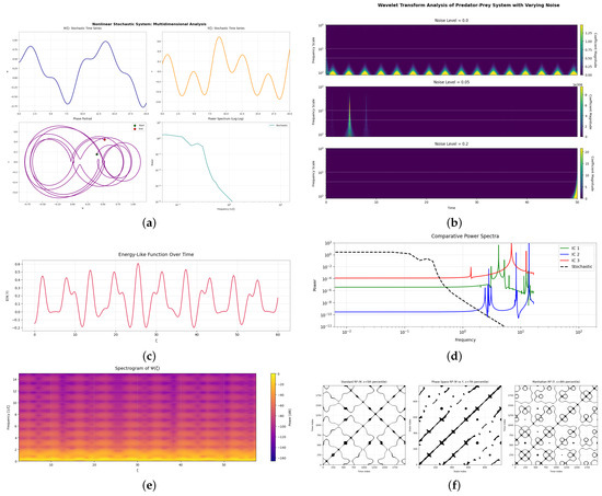
Figure 17.
Multi-panel visualization of nonlinear and stochastic dynamical behavior. Subfigures illustrate time series, phase-space trajectories, power spectra, wavelet and Fourier-based time-frequency analyses, energy evolution, and recurrence plots. Together, these provide a comprehensive view of how noise, nonlinearity, and system parameters influence temporal coherence, spectral structure, and phase-space complexity. (a) Multivariate time-series and phase-space dynamics. (b) Continuous wavelet transform (CWT) of under increasing noise levels ( = 0,0.1,0.2). (c) Time evolution of an energy-like quantity, possibly . (d) Comparison of power spectra across deterministic and stochastic variants. (e) Short-time Fourier spectrogram of . (f) Recurrence plots under different dynamical regimes.
5.5.1. Figure 17a
- Top Left: vs. time () shows a smooth but noisy trajectory, likely under stochastic forcing. Oscillations grow and decay, hinting at nonlinear interactions and dissipative effects.
- Top Right: Companion state variable shows less smooth dynamics, likely due to being the velocity or derivative of . Sharp oscillations suggest sensitivity to perturbations or high-frequency forcing.
- Bottom Left (Phase Portrait): The 2D trajectory ( vs. ) exhibits a complex, multi-loop structure indicative of a strange attractor. It is likely that simultaneously chaotic as well as quasiperiodic patterns of action will be present.
- Bottom Right (Power Spectrum): Broad spectral support is revealed by a log–log power spectral density (PSD), which has significant dynamical implications. Strong frequencies are indicated by distinct resonance peaks, whereas wandering or erratic motion, which is a feature of stochastic or chaotic dynamics, is reflected by a wide spectral spread. Furthermore, the existence of scale-invariant features points to power-law decay and fractal behavior in the underlying system.
5.5.2. Figure 17b
The wavelet analysis indicates that the energy time frequency has a distinct distribution across a range of noise levels. We observe clear periodic components with constant frequency in the deterministic system (), which is a characteristic of a non-perturbed nonlinear oscillator. The energy distribution is seen to become somewhat wider in each frequency direction when noise () is introduced to the signal. This phenomenon is linked to phase diffusion and timing jitter, but it does not significantly alter the signal’s original periodic nature. However, the system exhibits significant spectral variations when the noise level rises (), including the major energy blurs in reduced frequencies along with the temporal coordinated shifts to reduction in conjunction with the frequency drift effects. These stepwise time–frequency shifts demonstrate how the system’s periodic properties are gradually harmed by the increasing stochastic forcing, which also adds new dynamics. Therefore, if the oscillations are deterministic, the wavelet analysis provides a visual record of the noise-induced onset of stochastic-dominated dynamics.
5.5.3. Figure 17c
The quantity being plotted is , which is a derivative of a quantity that is most likely defined as the system’s total energy. The resulting observed behavior has oscillatory but strictly confined energy variations that establish the stability of the system and the fact that it has no divergent solutions. This vibrational phase portrait implies quasiperiodic behavior with either minimal damping, or energy-conserving energy transfer processes, in which injections of potential energy by external forcing or noise seem to overcome all the dissipative processes. The fact that these oscillations are bounded signals that the system is long-term stable in spite of the complex dynamics between the deterministic and the stochastic part of the system, as is typical of nonlinear systems within a stable dynamical regime.
5.5.4. Figure 17d
The dynamics of a three-variable stochastic system (black dashed line) is compared with three deterministic systems (IC1, IC2, IC3) that have initial conditions of , , and , respectively. In contrast to deterministic systems, which have sharp peaks, stochastic systems have a broad, continuous spectrum that is typical of chaos or noise-limited dynamics; these spectra serve as indicators of the dynamics’ quasiperiodic character. Compared to IC1, the deterministic systems IC2 and IC3 show more intense frequency structures and particularly strong harmonics, indicating more complex nonlinear dynamics. These observations demonstrate how deterministic systems with stronger nonlinearity or forcing parameters have more spectral content, while stochastic systems tend to smear these discrete characteristics into a spectral continuum, which is fundamentally against the nature of the system from a frequency-domain perspective.
5.5.5. Figure 17e
The short-time Fourier transform examination is used to view the time evolution of the system’s spectral content, revealing a number of significant dynamical features. It is evident that the spectrogram’s horizontal bands represent ongoing oscillatory modes with steady frequencies over time, while minor band drifts or fading indicate a slow loss of coherence or frequency modulation effects. The analysis reveals that mid-frequency modes with slight temporal variations in their spectral signatures dominate the system’s dynamics. It suggests that there may be sporadic resonance or weaker noise that subtly affects the system’s oscillatory behavior without changing its distinctive frequency components. The transform is thus able to capture the stagnant features of the spectrum as well as its finite time dynamics, which gives a clue to the dynamics in the system.
5.5.6. Figure 17f
Recurrence plots are an effective method of displaying the self-similar behavior patterns of the phase space, with the difference between the phase points belonging to different dynamical systems. The left panel shows crisp steady diagonal slopes typical of deterministic systems that are highly periodic so that trajectories are almost exactly repeated at different points in time. On the contrary, the middle plot has interrupted recurrence with seemingly either quasiperiodic or weak chaos, as shown by diverging trajectories. The right plot is a grid or fuzzy small structure seen in strongly nonlinear or stochastic systems having complex phase-space embedding and high-dimensional dynamics. The trends in these diagrams show the predictive power or the dimensional richness of a system in its structures of recurrence; that is, the extent of continuity and symmetry of recurrences directly corresponds to the predictability of a system—the higher the predictability, the more symmetric and contiguous their periodicities or structures of recurrence, and the more periodic a system, the more complex the measurements of these systems on each dimension of space and time are. Hence, highly predictable systems of periodicity are also highly dimensional. The recurrence analysis can therefore be used as a useful diagnostic tool to classify dynamics of systems in terms of their temporal correlation characteristics.
This section’s study provides a thorough exploration of a nonlinear dynamical system under deterministic and stochastic impacts through a combined diagnostic methodology which includes time-series, phase-space, spectral and recurrence investigations. The findings illustrate the interaction between nonlinearity and noise to cause changes in quasiperiodic order to chaotic and stochastic order, evidenced by broadening of spectrums, loss of coherence, and complexity of phase space. Still, with stochastic perturbations, the system is subjected to a finite energy and this means that the system is dynamically stable. Multimodal frameworks are a combination of geometric, spectral and topological measures, sensitive to both noise-induced transitions and changes in sensitivity and a generalizable approach to the analysis of real-world systems, including fluid oscillations, electronic circuits, climate models, and nonlinear and stochastic interactions are present.
6. Innovative Aspects and Contributions
Though the tools of analysis used in the paper, including spectral solvers, Darboux transformations, Lyapunov exponents and entropy-based measures, are all widely known, their combination in a single analytical–computational framework is an important milestone. The current paper is the first to present a unified approach to deterministic soliton dynamics with stochastic oscillator dynamics: here, coherent and dispersive waveforms are directly compared under the same forcing conditions. It is analyzed that the periodic and stochastic excitations are intertwined and critical thresholds are present where noise transforms stable solitons into stochastic attractors, and noise forms a two-sided role of dismantling and forming nonlinear structures. Also, it is shown that the OGY chaos control technique is extended to stochastic soliton regimes, providing a flexible and adaptive means of stabilization, which is able to maintain the coherence and structure of the waveforms when random perturbation is large. This generalization of classical deterministic methods of control has proved that noisy nonlinear dynamics can also be controlled and hence that it is possible to make soliton-based systems stronger and under control. Lastly, recurrence analysis, permutation entropy, and multidimensional embedding are ultimately integrated to offer a more sophisticated diagnostic procedure that highlights delicate changes in complexity and structure in deterministic and stochastic systems, making current dynamical studies apply to a larger and more natural category of nonlinear systems.
7. Conclusions
This comprehensive study has focused on the nonlinear systems defined by systems with Equations (6) and (5), which describe a class of periodically forced oscillators and wave-type models derived via Darboux transformations and nonlinear superposition principles. The term “nonlinear waveforms and oscillators” thus refers specifically to these systems, encompassing both soliton-bearing wave equations and the reduced oscillator dynamics governed by cubic and quadratic nonlinearities.
Soliton-like solutions were shown to exhibit marked stability compared to those of dispersive wave packets, which are more susceptible to numerical degradation. Through an integrated use of spectral solvers, Darboux transformations, Lyapunov exponents, power spectral analysis, recurrence plots, entropy measures, and multidimensional phase-space visualizations, we have traced the dynamical evolution from ordered quasiperiodic behavior to deterministic and stochastic chaos.
In the context of the forced oscillator System (5), it was demonstrated that variations in the parameters and the inclusion of stochastic forcing terms lead to transitions between periodic, quasiperiodic, and chaotic regimes. The results emphasize the role of nonlinearity in shaping amplitude modulation, frequency locking, and sensitivity to initial conditions.
Key findings reveal that initial conditions and waveform structures critically determine long-term stability and transitions to chaos. Noise, while typically expected to disrupt order, was found to induce semi-organized temporal structures under certain conditions, as evidenced by permutation entropy and recurrence-based diagnostics. In particular, we demonstrated that stochastic forcing does not merely increase disorder but can also introduce complex, structured behaviors, including resonant and bifurcation phenomena at critical noise intensities. This was confirmed by positive Lyapunov exponents and entropy peaks that identified noise-sensitive transitions and dynamic thresholds.
Moreover, comparison of deterministic and stochastic forms of System ((5)) revealed that stochastic perturbations preserve attractor boundedness while modulating temporal complexity. The systems often remain globally non-chaotic, with attractors maintaining their structural integrity even under moderate noise, highlighting the robustness of the underlying nonlinear potential.
Our analysis of nonlinear oscillators under periodic and stochastic forcing showed that the systems often remain bounded and non-chaotic, with attractors maintaining their structural integrity. Even under increasing noise, the underlying topology of the phase space remains stable, though temporal entropy increases moderately. The use of permutation entropy proved especially effective in revealing subtle variations in local complexity, complementing more traditional measures such as Shannon entropy and Lyapunov spectra.
Furthermore, the application of delay-coordinate embedding and attractor reconstruction emphasized the importance of selecting an optimal time delay. Small delays lead to redundancy, while excessively large delays obscure the system’s true dimensional structure. An intermediate delay—such as in the 3D case—allowed for faithful reconstruction and low-dimensional modeling of the system’s dynamics.
Hence, the study establishes a clear dynamical correspondence between the governing nonlinear oscillator equations and their soliton analogs, demonstrating how deterministic and stochastic forcing interact to shape long-term stability, coherence, and complexity in nonlinear physical systems.
Author Contributions
Conceptualization, A.J. and M.I.; methodology, A.J.; software, A.J.; validation, A.J. and M.I.; formal analysis, M.M.; investigation, M.M. and A.J.; resources, M.I.; data curation, A.J.; writing—original draft preparation, M.M.; writing—review and editing, A.J. and M.I.; visualization, M.M.; supervision, A.J.; project administration, A.J.; funding acquisition, A.J. and M.I. All authors have read and agreed to the published version of the manuscript.
Funding
This article has been produced with the financial support of the European Union under the REFRESH – Research Excellence For Region Sustainability and High-tech Industries project number CZ.10.03.01/00/22_003/0000048 via the Operational Programme Just Transition.
Data Availability Statement
The article contains all of the data that were analyzed for the current project.
Acknowledgments
M. Imran would like to express his sincere gratitude to Ajman University for the financial support and resources provided for this research under the Internal Research Grant No. DRG Ref. Number: 2025-IRG-CHS-17.
Conflicts of Interest
The authors declare that they have no conflicts of interest to report regarding the present study.
References
- Yin, L.; Agrawal, G.P. Impact of two-photon absorption on self-phase modulation in silicon waveguides. Opt. Lett. 2007, 32, 2031–2033. [Google Scholar] [CrossRef] [PubMed]
- Whitham, G.B. Linear and Nonlinear Waves; John Wiley & Sons: Hoboken, NJ, USA, 2011. [Google Scholar]
- Winfree, A.T. The Geometry of Biological Time; Springer: New York, NY, USA, 1980; Volume 2. [Google Scholar]
- Kivshar, Y.S.; Agrawal, G.P. Optical Solitons: From Fibers to Photonic Crystals; Academic Press: Cambridge, MA, USA, 2003. [Google Scholar]
- Remoissenet, M. Waves Called Solitons: Concepts and Experiments; Springer Science & Business Media: Berlin/Heidelberg, Germany, 2013. [Google Scholar]
- Hasegawa, A.; Kodama, Y. Solitons in Optical Communications; Oxford University Press: Oxford, UK, 1995. [Google Scholar]
- Dauxois, T.; Peyrard, M. Physics of Solitons; Cambridge University Press: Cambridge, UK, 2006. [Google Scholar]
- Shabat, A.; Zakharov, V. Exact theory of two-dimensional self-focusing and one-dimensional self-modulation of waves in nonlinear media. Sov. Phys. JETP 1972, 34, 62. [Google Scholar]
- Ablowitz, M.J.; Segur, H. Solitons and the Inverse Scattering Transform; Society for Industrial and Applied Mathematics: Philadelphia, PA, USA, 1981. [Google Scholar]
- Yang, J. Nonlinear Waves in Integrable and Nonintegrable Systems; Society for Industrial and Applied Mathematics: Philadelphia, PA, USA, 2010. [Google Scholar]
- Taha, T.R.; Ablowitz, M.I. Analytical and numerical aspects of certain nonlinear evolution equations. II. Numerical, nonlinear Schrödinger equation. J. Comput. Phys. 1984, 55, 203–230. [Google Scholar] [CrossRef]
- Ott, E. Chaos in Dynamical Systems; Cambridge University Press: Cambridge, UK, 2002. [Google Scholar]
- Strogatz, S.H. Nonlinear Dynamics and Chaos: With Applications to Physics, Biology, Chemistry, and Engineering; Chapman and Hall/CRC: Boca Raton, FL, USA, 2024. [Google Scholar]
- Pikovsky, A.; Rosenblum, M.; Kurths, J. Synchronization: A Universal Concept in Nonlinear Sciences; Cambridge University Press: Cambridge, UK, 2003. [Google Scholar]
- Kantz, H.; Schreiber, T. Nonlinear Time Series Analysis; Cambridge University Press: Cambridge, UK, 2003. [Google Scholar]
- Sauer, T.; Yorke, J.A.; Casdagli, M. Embedology. J. Stat. Phys. 1991, 65, 579–616. [Google Scholar] [CrossRef]
- Ott, E.; Grebogi, C.; Yorke, J.A. Controlling Chaos. Phys. Rev. Lett. 1990, 64, 1196. [Google Scholar] [CrossRef]
- Ablowitz, M.J.; Clarkson, P.A. Solitons, Nonlinear Evolution Equations and Inverse Scattering; Cambridge University Press: Cambridge, UK, 1991; Volume 149. [Google Scholar]
- Matveev, V.B.; Salle, M.A. Darboux Transformations and Solitons. In Springer Series in Nonlinear Dynamics; Springer: New York, NY, USA, 1991. [Google Scholar]
- Bandt, C.; Pompe, B. Permutation entropy: A natural complexity measure for time series. Phys. Rev. Lett. 2002, 88, 174102. [Google Scholar]
- Norbert, M.; Romano, M.C.; Thiel, M.; Kurths, J. Recurrence plots for the analysis of complex systems. Phys. Rep. 2007, 438, 237–329. [Google Scholar] [CrossRef]
- Guo, S.; Wu, J. Bifurcation Theory of Functional Differential Equations; Springer: New York, NY, USA, 2013; Volume 10, pp. 978–981. [Google Scholar]
- Pyragas, K. Continuous control of chaos by self-controlling feedback. Phys. Lett. A 1992, 170, 421–428. [Google Scholar] [CrossRef]
- Sarwar, S. New soliton wave structures of nonlinear (4+ 1)-dimensional Fokas dynamical model by using different methods. Alex. Eng. J. 2021, 60, 795–803. [Google Scholar] [CrossRef]
- Alhakim, L.; Gasmi, B.; Moussa, A.; Mati, Y.; Baskonus, H.M. Exploring bifurcation, phase portraits, and exact solutions of the Fokas equation using the improved Cham method. Partial. Differ. Equations Appl. Math. 2025, 13, 101134. [Google Scholar] [CrossRef]
- Almusawa, H.; Jhangeer, A.; Munawar, M. Analytical analyses for a fractional low-pass electrical transmission line model with dynamic transition. Symmetry 2022, 14, 1377. [Google Scholar] [CrossRef]
- Samina, S.; Munawar, M.; Ansari, A.R.; Jhangeer, A.; Wali, S. Nonlinear optical dynamics and complex wave structures in nonlinear dispersive media. Sci. Rep. 2025, 15, 15562. [Google Scholar] [CrossRef] [PubMed]
- Jhangeer, A.; Munawar, M.; Imran, M.; Kader, A.A. Chaotic demonstration of the twin-core couplers with Kerr law non-linearity employing beta derivative. Partial. Differ. Equations Appl. Math. 2025, 14, 101197. [Google Scholar] [CrossRef]


Disclaimer/Publisher’s Note: The statements, opinions and data contained in all publications are solely those of the individual author(s) and contributor(s) and not of MDPI and/or the editor(s). MDPI and/or the editor(s) disclaim responsibility for any injury to people or property resulting from any ideas, methods, instructions or products referred to in the content. |
© 2025 by the authors. Licensee MDPI, Basel, Switzerland. This article is an open access article distributed under the terms and conditions of the Creative Commons Attribution (CC BY) license (https://creativecommons.org/licenses/by/4.0/).