Abstract
Thermally characterizing high-thermal conductivity materials is challenging, especially considering high temperatures. However, the modeling of heat transfer processes requires specific material information. The present study addresses an inverse approach to estimate the thermal conductivity of SAE 1020 relative to temperature during an autogenous LASER Beam Welding (LBW) experiment. The temperature profile during LBW is computed with the aid of an in-house CUDA-C algorithm. Here, the governing three-dimensional heat diffusion equation is discretized through the Finite Volume Method (FVM) and solved using the Successive Over-Relaxation (SOR) parallelized iterative solver. With temperature information, one may employ a minimization procedure to assess thermal properties or process parameters. In this work, the Quadrilateral Optimization Method (QOM) is applied to perform estimations because it allows for the simultaneous optimization of variables with no quantity restriction and renders the assessment of parameters in unsteady states valid, thereby preventing the requirement for steady-state experiments. We extended QOM’s prior applicability to account for more parameters concurrently. In Case I, the optimization of the three parameters that compose the second-degree polynomial function model of thermal conductivity is performed. In Case II, the heat distribution model’s gross heat rate (Ω) is also estimated in addition to the previous parameters. Ω [W] quantifies the power the sample receives and is related to the process’s efficiency. The method’s suitability for estimating the parameters was confirmed by investigating the reduced sensitivity coefficients, while the method’s stability was corroborated by performing the estimates with noisy data. There is a good agreement between the reference and estimated values. Hence, this study introduces a proper methodology for estimating a temperature-dependent thermal property and an LBW parameter. As the performance of the present algorithm is increased using parallel computation, a pondered solution between estimation reliability and computational cost is achieved.
1. Introduction
Mathematical modeling is an essential tool for enhancing industrial processes, both for process control and product quality. Modeling heat transfer processes requires knowledge of the process parameters, the environmental attributes to define the boundary conditions, and the material characteristics, such as size, to define the domain and the thermophysical properties to adequately describe the heat transfer. In addition, the use of temperature-dependent properties substantially influences the validity of the simulation outcomes [1]. However, the materials properties are dictated by their chemical composition and the spatial arrangement of their components. Thus, such properties usually oscillate, given small differences in composition [2]. This fact hinders cataloging the properties of all materials, as new ones are being developed at different materials engineering branches [3,4,5,6,7].
There are direct approaches for attaining thermophysical properties. Besides consulting data series such as the Thermophysical Properties of Matter (TPRC), one may also measure such properties experimentally. Some thermal characterization methods consist of the guarded hot plate (GHP) [8,9], the LASER flash method [10,11], and the comparative fluxmetric method (CFM) [12]. However, precise material characterization usually involves large amounts of unknown parameters, which may vary with the temperature gradient. Also, the literature regarding low-temperature range and low-thermal conductivity materials is vast, but most approaches entail materials in the solid state. Indeed, there is a gap regarding metals at high temperatures, i.e., temperatures close to the melting point, because the data acquirement may be hampered due to the interactions between the specimen and its container, for example [13].
Then, inverse approaches are being extensively used to fill such a gap in obtaining the data on thermophysical properties. In this case, the inverse heat transfer problems (IHTPs) are applied to estimate unknown parameters of the thermal process, given temperature data inside or on the surface of the domain. The temperature information may be retrieved from numerical experiments, which determine the temperature based on a mathematical model, or from laboratory experiments, which usually focus on measuring the temperature field in specific points of a thermally excited sample [14,15]. Several areas of thermal engineering benefit from the inverse technique. For example, one may cite the estimation of the thermal conductivity of polymeric materials [16], the attainment of the unknown functional form of a time-dependent heat transfer coefficient [17], and the estimation of the thermal conductivity and volumetric heat capacity of living tissue using a recent noninvasive measurement method [18]. In addition, there are IHTP applications in food science and engineering for assessing process parameters, for example, the energy consumption during baking [19] or temperature-dependent food properties such as moisture diffusivity [20].
Besides the previous examples regarding the attainment of parameters from experimental or numerical temperatures, several different methods exist to optimize the parameters of interest. In [21], the authors acquired the numerical temperature of a metal sample interacting with a LASER pulse through the commercial software ANSYS Fluent ®. After validating the model with laboratory experiments, the authors applied the Levenberg–Marquardt (LM) technique to optimize four LASER pulse parameters: the power of the LASER pulse, the dimensionless shape parameter of the heat source distribution, and the beginning and end times of its interaction with the sample. The inverse algorithm was implemented by applying GNU Octave and ANSYS Fluent software packages. Another approach is to combine artificial intelligence with inverse heat conduction problems. In [22], the authors propose a proportional-integral-derivative (PID) inverse algorithm to perform the real-time estimation of the boundary heat flux in an unsteady heat conduction problem. To address the lack of adaptive ability of the latter method, the authors introduce the single neural adaptive PID (SNA-PID) [23]. Such a method is capable of adaptively adjusting the weights of the PID parameters and is more robust regarding signal interferences than the classical PID method. Both AI approaches comprise inverse the estimate of boundary heat flux involved in a numerical experiment governed by a one-dimensional transient heat diffusion equation, given the numerical data computed at a single position. Bayesian techniques, namely Gauss–Newton minimization regarding the maximum a posteriori objective function and the Markov chain Monte Carlo method application in the simultaneous assessment of the thermal diffusivity and thermal conductivity of a metallic sample were proved to be accurate [13]. Herein, the experimental setting based on the front-face flash method with contactless transient flux measurements of thermally excited metallic samples was modeled. The forward problem was solved through the Finite Element Method (FEM) with the aid of COMSOL Multiphysics® 4.3b, while the inverse problem analytical solution was implemented using MATLAB®. The Broydon–Fletcher–Goldfarb–Shanno (BFGS) technique consists of the minimization of an error square function, given the difference between the numerical and experimental temperatures. The latter approach could be successfully applied to attain the thermal profile from the estimated heat rate during Gas Tungsten Arc Welding (GTAW) [24]. Afterward, the methodology was applied to determine the cooling rate at the Fused Zone (FZ), Heat-Affected Zone (HAZ), and Base Metal (BM). The authors implemented the direct and inverse models in an authorial C++ software [25].
The main limitation of the previously reviewed works lies in properly optimizing the solution of inverse heat transfer problems by driving the forward model through an efficient optimization tool. Therefore, the present study showcases the application of a methodology developed to estimate a temperature-dependent thermal property by carefully balancing the solution between estimation reliability and computational cost, thereby addressing the gap in the literature. The applied multivariable optimization technique is the Quadrilateral Optimization Method (QOM) previously proposed by Magalhães [26], which enables the estimation of temperature-dependent thermal properties described by math functions. This inverse method was specifically developed to determine material thermal properties at elevated temperatures. A key advantage of the QOM is its ability to estimate parameters in unsteady states, eliminating the need for steady-state experiments. In the present work, the QOM functionality was extended to enable the simultaneous estimation of a higher number of parameters. The extension also allows for estimating different quantities other than thermal properties.
In this work, the QOM is applied to acquire the nonlinear thermal conductivity of an SAE 1020 sample and the heat input provided by the LASER during a LASER Beam Welding (LBW) process. The solution to the forward problem described in Section 2.1 is achieved using an in-house CUDA-C algorithm to attain the reference temperature evolution during 2.0 s of experiment. Here, the three-dimensional heat diffusion equation is discretized through the Finite Volume Method (FVM), and the thermal conductivity function used to model the property evolution with temperature presents a second-degree polynomial form. With possession of the temperature data, the QOM is applied to minimize an objective function, considering different combinations of the parameters of interest. Two cases are studied. In Case I, we optimize the three parameters that compose the thermal conductivity function. In Case II, we optimize the gross heat rate provided by the LASER, along with the thermal conductivity. Implementing the method in a parallelized structure allows the computations to be performed at an acceptable time, reducing computational costs compared to those of sequential approaches. Further information about the inverse technique and details about its application in the estimation of thermal conductivity are given in Section 2.2 and Section 2.3. Once the numerical data used as reference are noiseless, the study of the method’s suitability for estimating the parameters given noisy data is delineated in Section 2.4. Section 3 describes the methods used in the sensitivity analysis and discusses the results of the reduced coefficients. The study of the sensitivity allows for the calibration of the number of time steps that regularize the objective function. Both accuracy and computational time are pondered to attain the optimal time steps. Such investigation is explained in Section 4. Afterward, we discuss in Section 5 the method’s stability introduced in Section 2.4. After assuring the method is qualified to perform the estimations, the estimation results and the comparison between the numerical temperatures computed given reference and estimated parameters are presented in Section 6.
2. Materials and Methods
2.1. The Forward Model
The assessment of temperature-dependent thermal conductivity is an ill-posed inverse problem. In this instance, the baseline for the estimates is the temperature field during the LASER beam welding of steel SAE 1020. The nonlinear three-dimensional heat diffusion equation may describe the transient heat transfer during the process as follows:
where x, y, and z are the cartesian coordinates, λ(T) is the nonlinear thermal conductivity, T is the temperature, ġ is the generated heat source, H is the nonlinear enthalpy function, and t is the time. H is used to model the phase change and may be expressed as follows:
where f is the fraction of solid, defined by the Heaviside step function; Tm is the melting temperature; ρ is the specific mass; cp,s and cp,l are the nonlinear specific heat of the solid and liquid material, respectively; and L is the fusion latent heat.
The heat source assumes a Gaussian distribution above the sample surface. However, the barrier effect suffered by the LASER beam decreases the heat flux distribution as the penetration increases up to the coordinate h. In this case, the volumetric generated heat distribution (ġ) may be written as follows:
where Ω (=1000 W) is the gross heat rate; R (=0.50 mm) is the weld bead radius; u (=0.05 m/s) is the welding velocity; L (=40.00 mm) is the sample width (along the y-axis); and x, y, and z are the coordinates in the respective Cartesian axis. Such values are defined by calibrating the experimental configuration so the simulated and the experimentally observed weld bead geometry match [27].
The model considers boundary conditions of convection and radiation at the sample surfaces, described by the following:
where n is the normal direction on the domain boundaries, h(T) is the convection heat transfer function, T∞ (=20 °C) is the environment temperature, and σ is the Stefan–Boltzmann constant. The inferior surface of the specimen had its convection coefficient calculated through the empirical correlations of a heated inverted horizontal flat plate [28]. In the side surfaces, the correlation for a vertical flat plate was used [29]. Lastly, the free jet model for forced convection was applied to the top surface [29].
An in-house algorithm written in CUDA-C language solves Equation (1) by discretizing it through the Finite Volume Method (FVM) to achieve the temperature profile during LBW. The equation is applied over the domain depicted in Figure 1. The point P0 (0,0,0) represents the origin of the domain. The heat source is pointed at P1 (5,10,0) at the beginning of the experiment and moves 30 mm along the x-axis until point P2 (35,10,0). The dotted lines stand for the sample centerline, which coincides with the joint centerline. In addition, the blue and red arrows are placed in the specimen’s surfaces subjected to heat loss by natural and forced convection, sequentially, as specified after Equation (4). Here, the heat loss in the posterior surface is omitted for the sake of clarity.
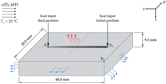
Figure 1.
Three-dimensional scheme of the simulated LBW process.
As shown in Equations (1) and (4), the thermophysical properties of the material are required to compute the temperature of the sample. Such inputs are temperature-dependent and accounted for as temperature functions with specific behavior. Regarding SAE 1020, the reference thermal conductivity data represented by the blue dots Figure 2. were retrieved from Clain et al. [30]. They may be modeled as a second-degree polynomial function of temperature, depicted as the orange dashed line, which is mathematically represented as . The maximum error between the reference information and the polynomial fitting is less than 4.5%, despite the outlier at circa 780 °C. Indeed, the steel presents an allotropic transformation near this temperature. In this model, the authors chose not to model such behavior with no prejudice toward the predicted temperature field for the sake of algorithm simplification and computational time savings.
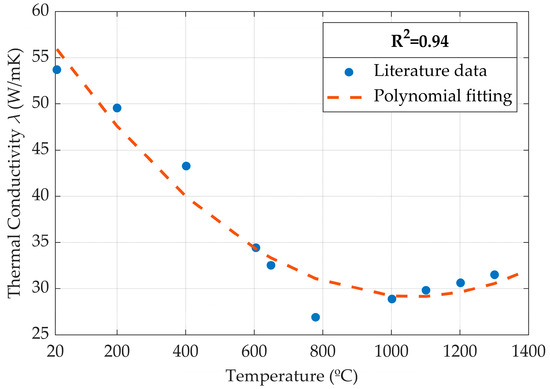
Figure 2.
Polynomial fitting of the nonlinear thermal conductivity function for SAE 1020.
A uniform orthogonal structured mesh with 225,000 total nodes (100 × 50 × 45 nodes, at x, y, and z, respectively) was applied in the solution of the forward model. The Finite Volume Method (FVM) system of equations was solved using the Successive Over-Relaxation (SOR) parallelized iterative solver. An energy residual convergence criterion was applied to all cases, and the threshold was set to 1.0 × 10⁻⁵. The applied simulation parameters are presented in Table 1.

Table 1.
Simulation parameters.
Solving the forward model through the in-house CUDA-C algorithm allows for the obtainment of the temperature profile shown in Figure 3. Each curve stands for the temperature evolution at a different point of the sample surface. The algorithm runs for an experiment period of 2.0 s, divided into 1.0 millisecond time steps. The thermocouples are placed at the same sample surface where the heat is applied (plane xy). The spots of temperature acquisition are exhibited in Table 2.
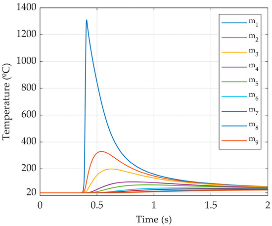
Figure 3.
Temperature evolution with the time during the autogenous LBW of SAE 1020.

Table 2.
Thermocouple positioning.
The forward model applied in this work underwent a rigorous verification process [31] to assess the quality of the resulting temperature fields. The verification steps involved investigations regarding the accuracy, computational performance, energy consumption, cost efficiency, and code memory optimization of the in-house CUDA-C code.
2.2. The Inverse Problem
The QOM developed by Magalhães [26] is an optimization method that allows for the assessment of more than one variable concurrently by minimizing an objective function (F) given by the sum of squares of the difference between the simulated (T’) and reference (T) temperatures. Moreover, F is minimized in a future time step rather than the present one to increase F sensitivity through the Future Time Regularization (FTR) [32]. This regularization technique expands the Function Specification Method developed by Beck et al. [33]. Thus, the regularized objective function may be described by the following:
where r is the number of time steps adopted, p is related to the time step position, N is the total number of thermocouples, and m is the thermocouple number.
Here, T is the numerical temperature computed using reference values of the assessed parameters, and T’ is the numerical temperature calculated using algorithm guesses, i.e., possible values of the parameters of interest. To define the values of each guess, the method divides a specified domain into 3κ equally distributed points, where κ is the number of parameters being assessed. Such a domain is addressed as the search domain and comprises all the possible linear combinations between the parameters, being limited by the maximum and minimum values each estimated parameter may assume. Then, the objective function is evaluated for each guess. The closer the assessed parameters are to the reference values, the closer T’ is to T, and, consequently, the objective function is lower. Therefore, the evaluation of F supports the definition of the pivot point Gp, being the guess that presents the minor objective function. A new set of 3κ guesses is distributed around the pivot point, following pre-defined convergence criteria, which decreases the domain at each interaction. The convergence process continues until the maximum number of interactions is reached. All the calculations are performed in an in-house CUDA-C code. In this case, the QOM algorithm proceeding may be summarized as follows:
- Initialize the number of variables (κ), convergence rate (τ), search domain bounds, maximum number of interactions, and number of time steps of the FTR;
- First division: evaluate the search domain bounds to define the initial guess vector G of equally spaced guesses within the domain;
- Settling the pivot point Gp: evaluate the objective function for each guess. The guess that presents the minimum F is defined as Gp;
- Redistribution: evaluate τ and Gp to redefine G with guesses equally far from Gp.
- Convergence: repeat steps 3 and 4 to decrease the domain at each interaction until the maximum number of interactions is reached.
The size of the initial domain division mentioned in step 2 may be determined for the general parameter ξ as follows:
where the subscripts 0 and 1 represent the minimum and maximum value the parameter ξ may assume, i.e., the search domain bounds.
As previously stated, the subsequent divisions of the domain are related to the pivot point instead of the upper and lower bounds as described in Equation (6). for the first division. In this instance, the size of the domain division (Δξ) decreases at each interaction by a factor c, given by the following:
where j is the counter for the interactions.
The convergence process continues until the maximum number of interactions is reached. At this point, the algorithm returns the combination of parameters of interest that present the lesser F, being the closest to the real values, as the difference between the temperature computed using such parameters (T’) and the reference temperature (T) is the minimum. An algorithm scheme is presented in Figure 4 for illustrative purposes.
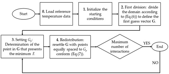
Figure 4.
Schematized procedure for the QOM algorithm.
2.3. QOM Applied to the Thermal Conductivity Estimate
Initially, the Quadrilateral Optimization Method is applied to simultaneously define the coefficients of the nonlinear thermal conductivity function of SAE 1020 (Case I). Then, the gross heat rate Ω used in the calculus of the heat distribution described in Equation (3) is estimated along with the nonlinear thermal conductivity function (Case II). To estimate the thermal conductivity using the heat transfer model described in Section 2.1, it is necessary to define all the parameters of the function that describes the nonlinear thermal conductivity. The reference thermal conductivity for SAE 1020 portrayed in Figure 2 may be represented by Equation (8).
Equation (9) shows the general form of λ(T), where the coefficients of the second-degree polynomial function (α, β, and γ) are real numbers that vary according to the sample composition. Hence, for the steel SAE 1020, the goal values the method should find for Equation (9) parameters α, β, and γ are 2.5×10⁻⁵, −5.3×10⁻², and 57.2, respectively.
Moreover, the estimation of the gross heat rate (Ω) along with the thermal conductivity function parameters requires the expansion of the algorithm so it minimizes all parameters concurrently. Such a parameter is constant (=1000 W), with no need for a function to model its behavior. In such a condition, four variables must be minimized at the same time. Regarding Ω, the goal value of 1000 W is obtained by the calibration of the forward model once it corresponds to the heat absorbed by the sample, given in Watts. Table 3 shows the definition of the search domain for estimating the thermal conductivity function parameters and the gross heat rate and summarizes the reference values. Besides defining the search domain, the method requires the convergence rate and maximum number of interactions. This work adopts τ = 0.5 and 16 interactions.

Table 3.
Conductivity function parameters and gross heat rate search domain.
In the search domain for Case I, the thermal conductivity function is within the three-dimensional plane defined by α, β, and γ, limited by the upper and lower bounds for each parameter. Hence, κ = 3, as there are three parameters of interest. For Case II, κ = 4 (α, β, γ, and Ω). For better clarification, we elucidate the search domain for Case I. In Figure 5, the edges defined by α, β, and γ are represented in red, blue, and green, respectively. For instance, point A coordinates are (α1, β1, and γ1), which correspond to (3.0 × 10⁻⁵, −5.0 × 10⁻², 80), according to Table 3. The gray dotted lines show the initial division of the domain into 43 equal cuboids. The divisions within the domain are omitted for better delineation. The inner cuboids dimensions are calculated by Equation (6).
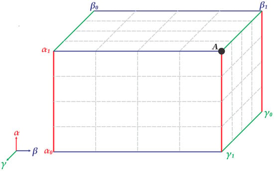
Figure 5.
Three-dimensional search domain for the thermal conductivity function parameters.
The guess vector G is defined by the divisions of the search domain, which correspond to specific combinations of α, β, and γ. When estimating three variables, each G is composed of 27 guesses, defined by the coordinates of the inner vertexes of the domain division. When estimating four parameters, 81 guesses are needed to account for the linear combinations between the parameters.
2.4. Input Data with Added Noise
The theory of linear propagation of uncertainty was applied in this work to extend the investigation and address the capabilities of the QOM when the input data contains added uncertainties and noise. Applying the theory of linear propagation of uncertainty results in [26]
where U is the global uncertainty, US’ is the uncertainty associated with experimental sensors, UT is the numerical thermal model uncertainty, and UQOM is the uncertainty related to the QOM approach. The US’ uncertainty term encompasses the temperature sensor positioning and the data acquisition system errors, as well as the thermal contact resistances involved in the measurements. The UT uncertainty includes the FVM, the solver truncation, and the numerical (rounding) errors. The UQOM term comprises the FTR uncertainty.
3. Sensitivity Analysis
In parameter estimation, it is necessary to investigate how expressive the parameter being assessed is for the calculated results. This investigation allows the verification of the method’s suitability for estimating such a parameter. The output from the forward model presented in Section 2.1 is the temperature profile during autogenous LBW. In light of this, this work evaluates the significance of temperature variation given a disturbance in the parameters α, β, γ, and Ω by analyzing the evolution of the sensitivity coefficients with time. The sensitivity coefficients may be obtained through the partial derivative of the temperature with respect to a specified parameter [34]. However, the unknown parameters may differ regarding the units or magnitude order. Hence, in order to standardize the coefficients, the reduced sensitivity coefficient (S) may be obtained by Equation (11), considering the assessment of the generic parameter X. In this instance, S is given in degrees Celsius.
Equation (11) represents the effect of the parameter X over the temperature, considering the temperature is acquired in one location. However, the direct model computes the temperature in the nine spots introduced in Table 2. Such configuration may be accounted for by summing the coefficients for every sensor as follows:
where Sn is the sensitivity coefficient for N sensors, and N is the number of thermocouples. In this case, N = 9.
We consider the significance of the temperature variation, given a 1% deviation in the model parameters, obtained by the central derivative of Equation (12), described by Equation (13).
3.1. Sensitivity of the Thermal Conductivity Function Parameters (α, β, and γ)
The significance of the temperature variation given a 1% disturbance in parameters α, β, and γ from the thermal conductivity function described in Equation (9) are portrayed in Figure 6. For all the parameters, the reduced sensitivity coefficient is equal or close to 0 from the beginning of the experiment until circa 0.200 s. The null values occur because there is no significant temperature variation during this period, so T = T∞ = 20 °C despite the parameters variations. After the constant period, Sn assumes positive values for about 0.1 s before dropping significantly. It corresponds to the pre-heating when the sample is subjected to a slight heat loss by convection, given the low temperature of the shielding gas jet. The sample temperature at all the considered spots should be greater than 20 °C when the coefficients start decreasing, assuming negative values from circa 0.400 s. Besides this behavior, every parameter investigated exerts significant influence on the temperature computed during the experiment, given the magnitudes of Sn. The most significant Sn values for α, β, and γ are −23.88, −51.75, and −86.02, respectively. Such values are found from 0.540 to 0.640 s. Therefore, the method is sensitive enough to assess the thermal conductivity function parameters, considering the temperature acquired by the nine sensors at the positions determined in Table 2.
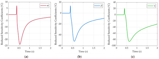
Figure 6.
Evolution of the thermal conductivity function parameters’ reduced sensitivity coefficients (Sn) with time. (a) α; (b) β; (c) γ.
3.2. Sensitivity of the Gross Heat Rate (Ω)
Figure 7 shows the evolution of the reduced sensitivity coefficient with the time for the gross heat rate. The parameter Ω exerts no influence on the temperature for the initial 0.300 s, corresponding to the period where the temperature difference is irrelevant. After that, the temperature variation given Ω increases at an enhanced rate for circa 0.1 s, and then the rate decreases. As previously stated, this time corresponds to the sample cooling by the action of the shielding gas, enhancing the heat transfer due to a more significant thermal gradient between the sample once its temperature is lower than 20 °C. When the sample temperature exceeds room temperature, the thermal gradient decreases, and so does the efficiency of the heat source. The most significant Sn for the gross heat rate is 111.7 °C, found at 0.573 s. The coefficients presented considerable values until the experiment ended.
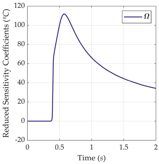
Figure 7.
Evolution of the gross heat rate reduced sensitivity coefficients (Sn) with time.
4. Future Time Regularization (FTR) Analysis
The objective function sensitivity is enhanced by the FTR, so F is calculated as described in Equation (5). Here, one may not calibrate the reference temperature T, which is constant in time and location, nor the numerical temperature T’, once the values result from the guesses automatically defined by the code. In this circumstance, one may attain more exact estimates by adjusting the number of time steps r or the number of thermocouples N or both. In order to evaluate the effect of different r on the assessments, this work considers the N constant (=9) once the Sn calculated using this thermocouple configuration presents acceptable values, as shown in Figure 6 and Figure 7.
Therefore, different numbers of time steps were applied to perform the estimates using the QOM. Here, the investigation of the relationships between r, the assessments accuracy, and the computational time required aims to attain the optimum number of time steps that should be considered for the parameter calculations. Considering the Sn calculated for α, β, γ, and Ω, it is possible to affirm the need for a considerable temperature variation so the method is sensitive enough to perform the estimates. In this case, the time considered for the calculations should be greater than the initial period where the temperature is comparable to 20 °C. The temperature profile depicted in Figure 3 implies that the temperature surpasses 20 °C close to 0.300 s. In order to determine the exact point in time where T > 20 °C for all the sensors, it is necessary to define such a point for the sensor placed farther away from the heat source. If the temperature at this point is greater than 20 °C during heating, the temperature at the other considered locations will also exceed 20 °C. Hence, Figure 8 shows the temperature profile for sensor m9 from 0 to 0.4 s. Here, the temperatures for the sensors m1 to m8 are omitted because the thermocouple m9 is farther from the heat source than the other sensors. The intersection between the dashed lines delimits the point in time from which the temperature assumes values greater than 20 °C. Therefore, more than 0.308 s should be used for the estimates. Moreover, it is possible to observe that the cooling caused by the shielding gas is less than 0.01 °C at this point.
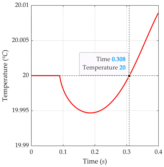
Figure 8.
Temperature profile at sensor m9 during 0.4 s.
The time and time step size ratio gives the number of time steps r. As the temperature is calculated at points 0.001 s from each other, r is given by the following:
So, to consider times over 0.308 s, one should apply r bigger than 308 to compute the objective function. Figure 9 highlights the Sn evolution for α, β, and γ from 0.3 to 0.6 s to guarantee the period Sn assumes considerable values. One may notice that the coefficients for all the parameters are unsuitable for the estimations at 0.308 s remaining close to 0 up to 0.350 s. To ensure that Sn is greater than the possible noise in the temperature data, we consider an absolute Sn of at least 5 °C appropriate. The α and β Sn are comparable to −5 °C at 0.410 s. However, the γ Sn passes such a value at 0.443 s. As all the parameters are appraised simultaneously, the lesser appropriate r is 443.
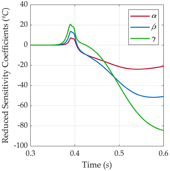
Figure 9.
Evolution of the reduced sensitivity coefficients (Sn) with time from 0.3 to 0.6 s for α, β, and γ.
In light of this, r values ranging from 450 to 900 were considered. The estimates obtained using the QOM, the reference values, and the error percentages are shown in Table 4. Also, the last column of the table refers to the objective function F obtained given the respective combination of α, β, and γ pondered by r. Such an assumption allows for the comparison of the data, disregarding the number of points summed. If the accuracy for each parameter was considered independently, the best r configuration would be 900 for α, 550 for β, and 800 or 850 for γ. However, by observing , it is possible to obtain the combination of α, β, and γ, for which the computed temperature is closer to the reference temperature. As all the parameters are assessed simultaneously, r = 450 should be applied.

Table 4.
Effect of the number of time steps in the estimates results.
In addition, the relationship between the computational time (t) required to perform the estimates and r is portrayed in Figure 10. In this period, the algorithm computes 432 times the direct model, given different combinations of α, β, and γ, and compares the results with the reference temperature to minimize the objective function, which is also calculated 432 times. Observing a linear proportion between the computational time required for the estimates and r is possible. The time varies because more or less temperature data are considered in the estimates. The dashed line stands for the linear trendline of the relationship between r and the time, described by Equation (15), with an R2 of 0.9994. The computational time ranges from 2760 to 5820 60 s. Thus, one should choose 450 r to estimate the thermal conductivity function parameters, as the estimates accuracy and computational time are satisfactory.
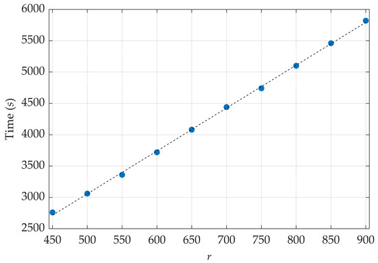
Figure 10.
Computational time for estimating α, β, and γ using the QOM with different r configurations.
Moreover, it is also possible to use r = 450 for Case II, given the expressive Sn for Ω until 0.450 s. The initial evolution of Sn with time is highlighted in Figure 11 for 0.300 to 0.450 s. The Sn exceeds 5 °C at 0.387 s, increasing to 83.6 °C at 0.450 s.
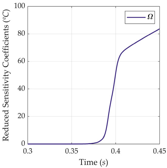
Figure 11.
Evolution of the reduced sensitivity coefficients (Sn) with time from 0.3 to 0.45 s for Ω.
5. Effect of Measurement Errors on the Estimated Results
Acquiring the temperature field using a numerical model implies no noise, measurement errors, or uncertainties once the computations are exact. However, experimental data could be used as a baseline for estimating materials thermal properties through the QOM, and possible temperature measurement errors may be enhanced in the estimation result, resulting in the method’s instability [23]. In this case, evaluating if the algorithm would return comparable results for noisy data is necessary. Hence, the QOM was applied to assess the parameters α, β, γ, and Ω given a disturbed temperature profile, as described in Section 2.4. The noise was added to the reference temperature profile (Figure 3) to verify if the method would return comparable results. A standard deviation of 10% was considered.
MATLAB® was used to add normalized random errors to the reference temperature. Such data were implemented in the algorithm as the reference temperature, considering the optimum r of 450. The results obtained by the QOM are shown in Table 5 for Cases I and II, as well as the error percentages for each parameter. One may notice that the errors remained lower than the imposed standard deviation for every parameter. Regarding Case I, there is a remarkable similarity between the values estimated with noisy data (Table 5) and the reference temperature (Table 4). This fact corroborates that the method is robust enough to perform the estimates, even if there is noise in the input data.

Table 5.
Estimated parameters and errors associated with noisy data.
6. Estimation Results
The estimations were performed by implementing the starting conditions described in Table 6. The results are presented in Section 6.1 and Section 6.2 for Cases I and II, respectively.

Table 6.
QOM algorithm parameters used in the estimations.
6.1. Case I: Nonlinear Thermal Conductivity Function
The estimated thermal conductivity in function of the temperature may be expressed as follows:
Note that such values for the parameters α, β, and γ were obtained when applying the optimal r configuration discussed in Section 4. When implementing Equation (16) in the direct model, the calculated temperature presents no significant deviations from the reference temperature during the experiment period at all thermocouples. Figure 12 shows good agreement between the data. In this matter, the numerical temperature profiles computed with the reference nonlinear thermal conductivity are represented by the solid lines, while the dotted lines depict the numerical temperature profiles acquired using the estimated nonlinear thermal conductivity function.
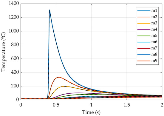
Figure 12.
Comparison between the numerical temperature profiles computed using the reference and the estimated nonlinear thermal conductivity function (Case I).
The relative error further analyzes the corroboration for the good agreement between the temperature. Table 7 describes the maximum deviation in percentages between the temperatures calculated when implementing Equations (8) and (16). It is possible to notice that the deviation is homogeneous for all the temperature acquisition spots, with an average of 2.46%.

Table 7.
Most expressive deviations between the numerical temperature profiles computed using the reference and the estimated λ(T) in terms of percent error.
6.2. Case II: Nonlinear Thermal Conductivity Function and Gross Heat Rate
The results obtained using the QOM to assess α, β, γ, and Ω and their respective error percentages are shown in Table 8.

Table 8.
Results attained for Case II applying 450 r.
Hence, the nonlinear thermal conductivity may be approximated by the following:
The dotted lines of Figure 13 represent the temperatures calculated using Equation (17) and Ω = 1071 W. It is possible to observe that the temperatures computed with the estimated thermal conductivity slightly overestimate the reference temperatures (solid lines). This tendency is found because the gross heat rate is 71 W greater than the reference value, so more heat is being provided to the sample, increasing its temperature. Regarding the peak temperatures, the more significant deviation is found at sensor m4, corresponding to less than 5% of the reference temperature. Hence, the estimated values of α, β, γ, and Ω are acceptable.
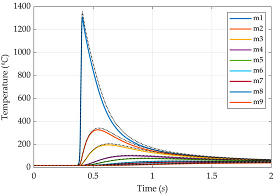
Figure 13.
Comparison between the numerical temperature profiles computed using the reference and the estimated nonlinear thermal conductivity function and the gross heat rate (Case II).
The magnitudes of the overestimates are depicted in Table 9, which shows the most significant error percentages when using Equations (8) and (17) to attain the temperature field. The error percentages are inversely proportional to the thermocouple distance to the heat source. As the overestimate is mainly due to the greater heat input, such a tendency emphasizes the more significant Ω effect in the temperatures calculated at positions near the heat source. Indeed, the temperature computed at m1 directly reflects the Ω magnitude. However, such an overestimate should not interfere with the experiment results, as it is insufficient to cause steel’s phase or microstructural changes during all experimental periods.

Table 9.
Most expressive deviations between the numerical temperature profiles computed using the reference and the estimated λ(T) and Ω in terms of percent error.
7. Conclusions
This work proposes an inverse method for estimating the thermal conductivity and gross heat rate during an autogenous LASER Beam Welding experiment. Two cases are considered. In Case I, we assess the three parameters that compose the second-degree conductivity function of temperature. In Case II, the gross heat rate related to the heat distribution is also estimated, in addition to the nonlinear thermal conductivity function. The temperature field is acquired by solving the three-dimensional heat diffusion equation using an in-house CUDA-C code. Such a language is also used to implement the inverse method. A gradient descendent technique called the Quadrilateral Optimization Method (QOM) is applied to optimize the parameters. The method’s suitability for Cases I and II is investigated by considering the sensitivity of the temperature for every parameter of interest and the stability of the method when performing the assessments from noisy data. After assuring the method is sensitive enough, we evaluate the effect of the number of time steps used in the regularization technique to optimize the estimates considering accuracy and computational time. The primary outcomes may be summarized as follows:
- The method is sensitive enough to provide precise estimates of the nonlinear thermal conductivity function and the gross heat rate simultaneously. The estimates consider nine points of temperature acquisition (see Table 2) during a 2.0 s experiment.
- The method sensitivity may be enhanced by calibrating the parameter r of the Future Time Regularization (FTR). The effect of r on the computational time and estimate accuracy was investigated. The optimum r that minimizes the computational time and presents considerable accuracy is 450.
- The comparison between the simulated temperature using reference and estimated values showed that the estimated parameters could be used as input data to calculate the heat transfer during SAE 1020 LBW. In Case I, the error remained lower than 3%. Case II presents more significant error percentages mainly due to the sensitivity of Ω. The values decrease from 11% with the sensor distance to the heat source.
- The computational time required for the estimates using 450 r is 46 1 min and 99 1 min for Cases I and II, respectively. In the former case, the direct model is calculated 432 times; in the latter case, the direct model is calculated 1296 times.
The results presented in this work emphasize the extent to which the QOM may be applied for IHTPs by performing the novel estimation of three and four parameters simultaneously, including both a thermophysical property and a process parameter. The main gaps of the adopted procedure consist of the requirement to know the functional form that best suits the modelization of property evolution with temperature. Also, the authors chose not to model the austenite decomposition of steel during solidification. One may also find slight differences when estimating the properties during the heating and cooling of the sample. Future works will address such behavior by considering different functions to model the thermal conductivity under determined temperature ranges. In addition, we intend to investigate the method’s sensitivity further by analyzing the amount and location of the thermocouples.
Author Contributions
Conceptualization, A.F.M.d.O. and E.d.S.M.; methodology, A.F.M.d.O., E.d.S.M. and P.L.M.; software, A.F.M.d.O., E.d.S.M. and E.J.G.d.N.; validation, A.F.M.d.O.; formal analysis, A.F.M.d.O.; investigation, A.F.M.d.O.; writing—original draft preparation, A.F.M.d.O.; writing—review and editing, A.F.M.d.O., E.d.S.M., P.L.M., K.D.Z. and E.J.G.d.N.; supervision, E.d.S.M., P.L.M. and K.D.Z.; project administration, E.d.S.M.; funding acquisition, E.d.S.M. All authors have read and agreed to the published version of the manuscript.
Funding
This research was funded by the Coordenação de Aperfeiçoamento de Pessoal de Nível Superior (CAPES) and by Petróleo Brasileiro S.A. (PETROBRAS).
Data Availability Statement
The data presented in this study are available on request from the corresponding author.
Acknowledgments
The authors would like to thank the Brazilian Ministry of Defense, the Brazilian Airforce (FAB), and the Aeronautics Institute of Technology (ITA).
Conflicts of Interest
The authors declare no conflicts of interest. The funders had no role in the design of the study; in the collection, analyses, or interpretation of data; in the writing of the manuscript; or in the decision to publish the results.
References
- Yan, S.; Meng, Z.; Chen, B.; Tan, C.; Song, X.; Wang, G. Prediction of Temperature Field and Residual Stress of Oscillation Laser Welding of 316LN Stainless Steel. Opt. Laser Technol. 2022, 145, 107493. [Google Scholar] [CrossRef]
- Zhao, S.; Sun, X.; Li, Z.; Xie, W.; Meng, S.; Wang, C.; Zhang, W. Simultaneous Retrieval of High Temperature Thermal Conductivities, Anisotropic Radiative Properties, and Thermal Contact Resistance for Ceramic Foams. Appl. Therm. Eng. 2019, 146, 569–576. [Google Scholar] [CrossRef]
- Belokon, Y.; Hrechanyi, O.; Vasilchenko, T.; Krugliak, D.; Bondarenko, Y. Development of New Composite Materials Based on TiN–Ni Cermets during Thermochemical Pressing. Results Eng. 2022, 16, 100724. [Google Scholar] [CrossRef]
- Panmanee, P.; Okhawilai, M.; Mora, P.; Jubsilp, C.; Karagiannidis, P.; Rimdusit, S. Development of a New Birthing Model Material Based on Silicone Rubber/Natural Rubber Blend. Polym. Test. 2023, 117, 107849. [Google Scholar] [CrossRef]
- Peng, G.; Sun, Y.; Zhang, Q.; Yang, Q.; Shen, W. A Collaborative Design Platform for New Alloy Material Development. Adv. Eng. Inform. 2022, 51, 101488. [Google Scholar] [CrossRef]
- Balandin, A.A.; Zaitsev-Zotov, S.V.; Grüner, G. Charge-Density-Wave Quantum Materials and Devices-New Developments and Future Prospects. Appl. Phys. Lett. 2021, 119, 17041. [Google Scholar] [CrossRef]
- Wardak, C.; Morawska, K.; Pietrzak, K. New Materials Used for the Development of Anion-Selective Electrodes—A Review. Materials 2023, 16, 5779. [Google Scholar] [CrossRef] [PubMed]
- Rottmann, M.; Beikircher, T.; Ebert, H.P. Thermal Conductivity of Evacuated Expanded Perlite Measured with Guarded-Hot-Plate and Transient-Hot-Wire Method at Temperatures between 295 K and 1073 K. Int. J. Therm. Sci. 2020, 152, 106338. [Google Scholar] [CrossRef]
- Jannot, Y.; Remy, B.; Degiovanni, A. Measurement of Thermal Conductivity and Thermal Resistance with a Tiny Hot Plate. High Temp. -High Press. 2010, 39, 11–31. [Google Scholar]
- Katz, M.D.; Katz, I.M. Evaluation of the Laser-Flash Method and Its Errors for Determining of Materials Thermal Diffusivity at High Temperatures. MATEC Web Conf. 2017, 110, 5. [Google Scholar] [CrossRef]
- Nishi, T.; Shibata, H.; Ohta, H.; Waseda, Y. Thermal Conductivities of Molten Iron, Cobalt, and Nickel by Laser Flash Method. Metall. Mater. Trans. A 2003, 34, 2801–2807. [Google Scholar] [CrossRef]
- Jannot, Y.; Meulemans, J.; Schick, V.; Capp, M.; Bargain, I. A Comparative Fluxmetric (CFM) Method for Apparent Thermal Conductivity Measurement of Insulating Materials at High Temperature. Int. J. Thermophys. 2020, 41, 94. [Google Scholar] [CrossRef]
- Lamien, B.; Le Maux, D.; Courtois, M.; Pierre, T.; Carin, M.; Le Masson, P.; Orlande, H.R.B.; Paillard, P. A Bayesian Approach for the Estimation of the Thermal Diffusivity of Aerodynamically Levitated Solid Metals at High Temperatures. Int. J. Heat Mass Transf. 2019, 141, 265–281. [Google Scholar] [CrossRef]
- Reddy, K.S.; Jayachandran, S. Investigations on Design and Construction of a Square Guarded Hot Plate (SGHP) Apparatus for Thermal Conductivity Measurement of Insulation Materials. Int. J. Therm. Sci. 2017, 120, 136–147. [Google Scholar] [CrossRef]
- El-Sharkawy, A.A.; Dessouky, M.T.; Abousehly, A.M.; Raafat, A. Thermal Properties Investigation of Inhomogeneous Ternary Alloy (Se–Te–S) Using Flash Method Technique. Int. J. Thermophys. 2020, 41, 25. [Google Scholar] [CrossRef]
- Farahani, S.D.; Kisomi, M.S. Experimental Estimation of Temperature-Dependent Thermal Conductivity Coefficient by Using Inverse Method and Remote Boundary Condition. Int. Commun. Heat Mass Transf. 2020, 117, 104736. [Google Scholar] [CrossRef]
- Mohebbi, F.; Sellier, M. Estimation of Functional Form of Time-Dependent Heat Transfer Coefficient Using an Accurate and Robust Parameter Estimation Approach: An Inverse Analysis. Energies 2021, 14, 5073. [Google Scholar] [CrossRef]
- Yue, K.; Zhang, X.; Yu, F. Simultaneous Estimation of Thermal Properties of Living Tissue Using Noninvasive Method. Int. J. Thermophys. 2007, 28, 1470–1489. [Google Scholar] [CrossRef]
- Ravula, S.R.; Arepally, D.; Datta, A.K. Estimation of the Energy Requirement of Bread during Baking by Inverse Heat Transfer Method. J. Therm. Anal. Calorim. 2023, 148, 13297–13311. [Google Scholar] [CrossRef]
- Cevoli, C.; Panarese, V.; Catalogne, C.; Fabbri, A. Estimation of the Effective Moisture Diffusivity in Cake Baking by the Inversion of a Finite Element Model. J. Food Eng. 2020, 270, 109769. [Google Scholar] [CrossRef]
- Łapka, P.; Pietrak, K.; Kujawińska, M.; Malesa, M. Development and Validation of an Inverse Method for Identification of Thermal Characteristics of a Short Laser Pulse. Int. J. Therm. Sci. 2020, 150, 106240. [Google Scholar] [CrossRef]
- Wan, S.; Xu, P.; Wang, K.; Yang, J.; Li, S. Real-Time Estimation of Thermal Boundary of Unsteady Heat Conduction System Using PID Algorithm. Int. J. Therm. Sci. 2020, 153, 106395. [Google Scholar] [CrossRef]
- Wan, S.; Wang, K.; Xu, P.; Huang, Y. Numerical and Experimental Verification of the Single Neural Adaptive PID Real-Time Inverse Method for Solving Inverse Heat Conduction Problems. Int. J. Heat Mass Transf. 2022, 189, 122657. [Google Scholar] [CrossRef]
- dos Santos Magalhães, E.; de Carvalho, S.R.; Silva, S.M.M.L.E. The Use of Non-Linear Inverse Problem and Enthalpy Method in GTAW Process of Aluminum. Int. Commun. Heat Mass Transf. 2015, 66, 114–121. [Google Scholar] [CrossRef]
- Magalhães, E.D.S.; Correa, E.O.; Silva, A.L.F.L.E.; Silva, S.M.M.L.E. Microstructural Analysis in GTA Aluminum Alloy Welding Using Inverse Problems. Appl. Therm. Eng. 2016, 100, 333–339. [Google Scholar] [CrossRef]
- Magalhães, E. dos S. A Quadrilateral Optimization Method for Non-Linear Thermal Properties Determination in Materials at High Temperatures. Int. J. Heat Mass Transf. 2021, 181, 121857. [Google Scholar] [CrossRef]
- de Oliveira, A.F.M.; Magalhães, E.D.S.; Paes, L.E.D.S.; Pereira, M.; da Silva, L.R. A Thermal Analysis of LASER Beam Welding Using Statistical Approaches. Processes 2023, 11, 25. [Google Scholar] [CrossRef]
- Çengel, Y.A.; Ghajar, A.J. Heat and Mass Transfer: Fundamentals and Applications, 4th ed.; McGraw-Hill Science/Engineering/Math: New York, NY, USA, 2010. [Google Scholar]
- Bergman, T.L.; Lavine, A.S.; Incropera, F.P.; Dewitt, D.P. Fundamentals of Heat and Mass Transfer, 7th ed.; John Wiley & Sons: Hoboken, NJ, USA, 2011. [Google Scholar]
- Clain, F.M.; Teixeira, P.R.D.F.; Araújo, D.B.D. Two Heat Source Models to Simulate Welding Processes with Magnetic Deflection. Soldag. E Insp. 2017, 22, 99–113. [Google Scholar] [CrossRef]
- Nascimento, E.; Magalhães, E.; Azevedo, A.; Paes, L.E.S.; Oliveira, A. An Implementation of LASER Beam Welding Simulation on Graphics Processing Unit Using CUDA. Computation 2024, 12, 83. [Google Scholar] [CrossRef]
- Magalhães, E.D.S.; Anselmo, B.D.C.S.; Lima e Silva, A.L.F.D.; Lima e Silva, S.M.M. Time Traveling Regularization for Inverse Heat Transfer Problems. Energies 2018, 11, 15. [Google Scholar] [CrossRef]
- Beck, J.V.; Blackwell, B.; Haji-Sheikh, A. Comparison of Some Inverse Heat Conduction Methods Using Experimental Data. Int. J. Heat Mass Transf. 1996, 39, 3649–3657. [Google Scholar] [CrossRef]
- Taktak, R.; Beck, J.V.; Scott, E.P. Optimal Experimental Design for Estimating Thermal Properties of Composite Materials. Int. J. Heat Mass Transf. 1993, 36, 2977–2986. [Google Scholar] [CrossRef]
Disclaimer/Publisher’s Note: The statements, opinions and data contained in all publications are solely those of the individual author(s) and contributor(s) and not of MDPI and/or the editor(s). MDPI and/or the editor(s) disclaim responsibility for any injury to people or property resulting from any ideas, methods, instructions or products referred to in the content. |
© 2024 by the authors. Licensee MDPI, Basel, Switzerland. This article is an open access article distributed under the terms and conditions of the Creative Commons Attribution (CC BY) license (https://creativecommons.org/licenses/by/4.0/).