The MLDAR Model: Machine Learning-Based Denoising of Structural Response Signals Generated by Ambient Vibration

Abstract

Engineers have consistently prioritized the maintenance of structural serviceability and safety. Recent strides in design codes, computational tools, and Structural Health Monitoring (SHM) have sought to address these concerns. On the other hand, the burgeoning application of machine learning (ML) techniques across diverse domains has been noteworthy. This research proposes the combination of ML techniques with SHM to bridge the gap between high-cost and affordable measurement devices. A significant challenge associated with low-cost instruments lies in the heightened noise introduced into recorded data, particularly obscuring structural responses in ambient vibration (AV) measurements. Consequently, the obscured signal within the noise poses challenges for engineers in identifying the eigenfrequencies of structures. This article concentrates on eliminating additive noise, particularly electronic noise stemming from sensor circuitry and components, in AV measurements. The proposed MLDAR (Machine Learning-based Denoising of Ambient Response) model employs a neural network architecture, featuring a denoising autoencoder with convolutional and upsampling layers. The MLDAR model undergoes training using AV response signals from various Single-Degree-of-Freedom (SDOF) oscillators. These SDOFs span the 1–10 Hz frequency band, encompassing low, medium, and high eigenfrequencies, with their accuracy forming an integral part of the model’s evaluation. The results are promising, as AV measurements in an image format after being submitted to the trained model become free of additive noise. This with the aid of upscaling enables the possibility of deriving target eigenfrequencies without altering or deforming of them. Comparisons in various terms, both qualitative and quantitative, such as the mean magnitude-squared coherence, mean phase difference, and Signal-to-Noise Ratio (SNR), showed great performance.

1. Introduction

Structural Health Monitoring (SHM) has become an intriguing topic during the last decades and is applied to various fields of civil, mechanical, automotive, and aerospace engineering, among others. Estimating the health condition and understanding the unique characteristics of structures by assessing the measured physical parameters in real time represents a major objective of SHM. As a result, signal processing has become an essential and inseparable part of methodologies introduced via research related to SHM. The application of signal processing techniques to the structural damage identification procedure is classified into two types of approaches, namely, (i) time-domain and (ii) frequency-domain methods. Experimental studies have assessed the potential of signal processing techniques in the two aforementioned domains, aiming to enhance vibration-based structural damage detection subjected to environmental effects (earthquakes, wind, etc.).

Although multiple review studies have been published on vibration-based structural damage detection, there have been no studies on categorizing signal processing techniques based on feature extraction procedures that belong to time and frequency domains for SHM purposes. Recently, this was explored in the work by Zhang et al. [1]. Meanwhile, with the developments in the classical SHM approach, neural networks and big data analytics have paved the way for a new approach in the field of SHM. As Zinno et al. [2] showcased with their work, Artificial Intelligence (AI) could benefit SHM applications for bridge structures in several phases: construction, development, management, and maintenance. Moreover, buildings are aging, and deriving newer architectural trends while preserving building heritage is not only of high value but also a complex procedure requiring multi-criteria approaches to decision making to be implemented [3]. Therefore, AI-based methodologies specially tailored to assist the preservation of building heritage through SHM techniques have already been developed and are summarized in the work by Mishra [4]. Generally speaking, one of the most common implementations of deep learning methodologies in SHM applications relies on the convolutional neural network (CNN) architecture; a summary of these can be found in the recent work by Sony et al. [5]. As is mentioned in the conclusion of the aforementioned work, one of the targets of future research will be the development of the real-time implementation of CNN-based approaches in everyday SHM practice; the model presented in the current work was developed for real-world practice. CNN-based models have already been applied with great success in different scientific fields, e.g., the work by Xu et al. [6], which also inspired the authors to develop the model presented in the current study; more specifically, in the work by Xu et al. [6], a CNN and a Recurrent Neural Network (RNN) were combined in order to dynamically detect levels of ambient noise from speech gaps and remove them from audio signals without distorting the speech audio quality. Also, during the last decades, multiple Deep Learning models have found a successful place in the denoising task for various noisy images. An overview about this can be seen in Elad et al.’s [7] work and Izadi et al.’s [8] work. In a recent investigation, Damikoukas and Lagaros [9] explored the feasibility of utilizing an ML model as a robust tool to predict building earthquake responses, addressing the shortcomings of simplified models. The study advanced by integrating AV measurements and earthquake time-history data into a neural network framework. This innovative model presents a promising pathway to deepen our comprehension of structural behavior in the face of seismic events, thereby contributing to the advancement of earthquake resilience in building design and engineering. Other recent works that tried to take advantage of neural networks in structural engineering and seismic response estimation are those of Xiang et al. [10] and Demertzis et al. [11].

The motivation behind this research was to delve into the potential of Deep Learning in addressing denoising challenges associated with Micro-Electromechanical System (MEMS) digital sensors, specifically accelerometers. This category of sensors is notable for its cost-effectiveness compared to alternatives like force balance accelerometers. However, they often contend with elevated levels of electronic noise. Recognizing the ongoing strides in AI capabilities and their ubiquitous integration into various domains, the motivation behind this work was to leverage Deep Learning for denoising tasks, laying the groundwork for more advanced applications, such as the real-time denoising of acceleration time histories. MEMS digital sensors, while economically advantageous, can suffer from inherent electronic noise. This noise can compromise the accuracy of measurements, especially in dynamic applications like acceleration monitoring. By harnessing the power of Deep Learning, this research aims to effectively mitigate this noise and enhance the reliability of sensor outputs. The broader context lies in the rapid evolution of AI technologies, which are progressively becoming integral components of everyday applications. This research envisions the deployment of Neural Processing Unit (NPU) hardware at the measurement site, paving the way for the real-time denoising of acceleration time histories. This not only addresses current challenges but also anticipates future scenarios where advanced techniques are seamlessly integrated into the measurement process. The utilization of NPUs represents a strategic move toward decentralized processing, enabling on-site denoising without relying solely on external computational resources. As a result, this research endeavors to contribute to the practical implementation of AI-driven denoising techniques, fostering advancements in the field of sensor technology and real-time data processing.

The achievement of this study is that ambient vibration (AV) measurements are processed through a properly calibrated neural network (NN) in an image format, and the structural response is unveiled after removing the additive electrical noise from the AV recordings. To train the model, 1197 structural oscillators (models of Single Degree of Freedom (SDOF)) were developed, from which 10,773 numerically produced noisy signals were generated. These signals were converted into images in order to be fed to the NN-based model chosen for the purposes of this study. For validation purposes, the results were converted back to numerical values in order to assess the level of denoising, among other factors, in terms of frequency spectra between predicted and target signals. The proposed model is called MLDAR, which stands for Machine Learning-based Denoising of Ambient Response.

The main contributions of this paper are (i) the denoising of ambient vibration (AV) acceleration measurements (ii) by presuming the structural eigenfrequencies in domain spectra needed for further structural analysis and assessment, all of which are realized by (iii) exploiting the power of neural networks (NNs) and Deep Learning (DP) deploying a multi-convolutional and transposed convolutional network.

The remainder of this paper is organized as follows. Section 2 generally describes the characteristics of the structural response generated by ambient vibration, how research on SHM during the last several decades has been progressing, and how new technologies are finding their fit due to their versatility and cost efficiency. In Section 2, the structural parameters used for the creation of the dataset are also presented, along with the list of the assumptions implemented. Afterward, Section 3 introduces the Machine Learning-based Denoising of Ambient Response (MLDAR) model, the basic principles on which it was based on, and also all the chosen parameters of its structure. Thereafter, Section 4 showcases the validation results of the proposed MLDAR model, both qualitative and quantitative. The paper concludes with some final remarks given in Section 5 and insights into the authors’ future work.

2. Structural Response Due to Ambient Vibration and SDOF Models

In this section, the characteristics of the structural response generated by means of ambient vibration is provided, together with the details of the models used to calibrate the neural network model developed for the purposes of this study.

2.1. Structural Response Generated by Ambient Vibration

Structures are permanently induced by various types of site excitations, which refer to either ground vibrations related to nature, e.g., earthquake genesis, or those generated by humans, like the vibrations generated during excavations, traffic, construction works, etc. Thus, structures continuously vibrate due to the above-mentioned causes, offering the possibility of monitoring and studying the structural response permanently. The structural response is of high value for structural engineers, as, among other tasks, they can derive the dynamic characteristics of the structure through the measurements they collect. Structural Health Monitoring (SHM) is a field where multiple sensors are deployed in order to enable engineers to monitor and assess the structural integrity, assist in deciding which interventions should be implemented, or even be alerted to an event, either at the precautionary or post-event state (early warning, etc.).

As nowadays, advancements in the manufacturing and technology of sensors and microcontrollers are huge, more and more sensing devices are released without any discounts on the level of their quality, shifting SHM research away from the traditional wired acceleration-sensing systems [12,13,14,15]. Meanwhile, attempts to broaden the use of SHM have been made, as more and more standards and design codes are being revised where SHM appears as an option or as an obligation for the engineers [16,17,18,19]. Therefore, there is an opportunity to ease any disadvantages of low-cost monitoring devices in terms of their implementation in civil engineering projects, bringing SHM into the mainstream of the structural engineering profession.

A common disadvantage of low-cost sensing devices is the higher level of noise that is introduced into the measurements. This noise is the additive distortion of the true-value signals. When it comes to high-magnitude motions, it is not an issue, as the real values can be acquired and processed easily. However, when we are referring to the ambient response of structures, the magnitude scale is really small, even smaller than today’s low-cost accelerometers’ level of noise. Therefore, in order to make use of noisy measurements in various algorithms and methodologies, time-domain dynamic quantities are usually skipped in favor of frequency-domain ones, such as eigenfrequencies. There are various data processing techniques that unveil information hidden by noise, such as the averaging of Fourier Spectra (e.g., [20]) and the recent work by the authors [21]. As said before, in the time domain, little can be done when measurements are already “noisy”, and here comes the current work to fill the gap, taking advantage of the power of neural networks and their image detection capabilities.

2.2. Models Used for Calibrating the NN

Neural networks, in order to be designed and trained, need both parameters of a system: input(s) and output(s). From that point on, after we decide properly what architecture we want and correctly configure every parameter, they can learn all those complex relationships between the prediction and what we have as input data. In this work, the approach is straightforward, as the aim is to train the neural network to distinguish additive noise from a noisy signal, which includes an ambient vibration structural response, and remove it in order to return a “clean” ambient vibration structural response signal. In order to do this, we would ideally need the “clean” and “noisy” versions of lots of response signals for different kinds of sensors and buildings. As that is not something easily feasible, we decided to start building the network from the ground up, using numerical data that corresponds to a batch of assumptions made both for sensor specifications and for the building models themselves.

Therefore, all data/measurements used were numerically generated and computationally derived from Newmark numerical integration. The reason was that we wanted to cover a whole range of SDOF oscillators, with all the possible different parameters’ combinations. In total, 1197 oscillators were used for the purposes of this study. The assumptions used to construct these oscillators were based on the model building that can be seen in Figure 1. The dimensions and other properties of the model building are specifically representative of the floor plan typically found in residential concrete buildings in Greece. This deliberate choice ensures that our study is grounded in a context reflective of prevalent architectural norms in the region, contributing to the relevance and applicability of our findings within the specified context. This model was constructed in the ADINA analysis software [22].

ADINA stands as a versatile software package renowned for its extensive capabilities in finite element analysis (FEA) and computational fluid dynamics (CFD). Tailored to address a diverse array of engineering challenges spanning multiple disciplines, ADINA excels in solving problems related to structural mechanics, heat transfer, fluid dynamics, electromagnetics, and multiphysics simulations. The acronym “ADINA” itself encapsulates its core functionality, representing “Automatic Dynamic Incremental Nonlinear Analysis”. As a comprehensive tool, ADINA’s strength lies in its ability to perform intricate simulations, offering engineers and researchers a robust platform for tackling complex problems in fields ranging from structural engineering to fluid dynamics. The software’s broad applicability makes it an invaluable resource for professionals seeking accurate and efficient solutions across various domains of engineering. ADINA’s prowess in dynamic, incremental, and nonlinear analyses underscores its suitability for simulating real-world scenarios, where the interactions between components and materials exhibit complex and dynamic behavior. By seamlessly integrating these capabilities, ADINA empowers users to gain deeper insights into the performance of their designs, aiding in the optimization of structures, processes, and systems. In essence, ADINA stands at the forefront of engineering simulation software, providing a sophisticated and adaptable suite of tools for addressing the multifaceted challenges inherent in the realm of finite element analysis and computational fluid dynamics. The number of assumptions and parameters used are shown in

Table 1. Model parameters.

Geometry
Plan	10.00 × 7.00 (m2)
Stories	1 to 7
Story height	3.50 (m)
Slab thickness	0.25 (m)
Columns	0.50 × 0.50 (m2)
Beams	0.40 × 0.70 (m2)
Loads
Dead	806.75 (kN)
Live	806.75 (kN)
Safety factor	1 1
Dynamic characteristics
Mass (per story)	110.78 (tons)
Damping ratio $\zeta$	5%
Eigenfrequency	1 to 10 Hz with step of 0.5
Material
Reinforced concrete
Bilinear material	Figure 2
Yield point	0.0105 m 2
Post-yield stiffness	50% of geometric one 3

¹ Assessment of existing conditions—real loads; ² 0.003 drift × 3.50 m = 0.0105 m (HazusC3L—LowCode). More details can be found in Hazus^®–MH 2.1 Technical Manual (see Paragraph 5.2.1 of [23]); ³ EC8–1 ($K_e=0.5K_g$). After first yield, loading is still happening with $K_{eff}$, even for small forces than $F_y$.

.

Figure 2 depicts the bilinear capacity curve used for all structural members. For each structural element, we considered two distinct stiffness states: geometrical stiffness, denoted by $K_g$, and effective stiffness, represented by $K_{eff}$. The effective stiffness, $K_{eff}$, is assumed to be half of the geometrical stiffness ($K_g$) and arises from the degradation experienced by the member under deformation, particularly in conditions of higher loads. This dual representation of stiffness allows for a more nuanced understanding of the structural response. The geometrical stiffness, $K_g$, captures the inherent stiffness of the member in its ideal, undistorted state, while the effective stiffness, $K_{eff}$, accounts for the impact of deformations and degradation induced by higher loads. By acknowledging the dynamic interplay between these two stiffness states, the model provides a more accurate and comprehensive depiction of the member’s behavior under varying conditions, facilitating a more realistic simulation of structural performance.

The numerically created ambient acceleration responses of the building’s models are noiseless, as they would be measured in an ideal experimental world, where measuring devices do not interfere in the slightest with measurable quantities. However, in real-world engineering applications, not only quantities are recorded by means of monitoring devices, as they are accompanied by various levels of noise, such as electronic noise. This family of noises is mathematically described as white noise, and statistically, it follows a normal distribution, with an average value of zero and a standard deviation related to the noise levels of the corresponding measuring device. The Signal-to-Noise Ratio (SNR), Noise Density (e.g., $\mathsf{\mu }\mathrm{g}/\sqrt{\mathrm{H}\mathrm{z}}$), and others are terms that usually describe the levels of noise in the recorded signals.

The final signals are the result of the sum of the aforementioned signals. The sampling rate is 100 Hz, and the duration of the artificial recordings is 60 s. Each building model consists of 1 to 7 floors, with a mass ranging between 80% and 120% of the aforementioned typical values (see Table 1) and with an eigenfrequency ranging between 1 and 10 Hz with a step of 0.5 Hz. Therefore, 1197 models of single-stage oscillators were derived. For each of these models, there are three signal windows of the theoretically no-(additional)-noise response and three electronic and non-electronic noise signal windows, which, superpositioned, lead to nine combinations of final response signals (pure oscillator response + electronic/other noise). Thus, 10,773 artificial signals were generated, which were converted into images and were the input of the machine learning model. They were created in the Matlab environment (release R2021b [24]). Of the generated signals, 75% were used for training (training set), while the other 25% were the validation sample (validation set).

3. Machine Learning-Based Models: Architecture and Calibration

During the last decade, due to the advances achieved in computer technology, machine learning has become very popular, having been applied with great success in different scientific areas, like autonomous vehicles, visual recognition, news aggregation and fake news detection, robotics, natural language processing, vocal Artificial Intelligence (AI), etc. Convolutional neural networks (CNNs) represent a class of artificial neural networks (ANNs) most commonly used for analyzing images. What makes them unique is that the network learns to optimize the filters (or kernels) through automated learning, whereas in traditional algorithms, these filters are hand-engineered. This independence from prior knowledge and human intervention in feature extraction is a major advantage. CNNs have applications in image and video recognition, recommender systems, image classification, image segmentation, medical image analysis, natural language processing, brain–computer interfaces, and financial time series.

3.1. Convolutional Neural Networks

Convolutional networks (e.g., LeCun et al. [25]), also known as convolutional neural networks, or CNNs, are a specialized kind of neural network for processing data that has a known grid-like topology. Examples include time-series data, which can be thought of as a 1-D grid taking samples at regular time intervals, and image data, which can be thought of as a 2-D grid of pixels. Convolutional networks have been tremendously successful in practical applications. The name “convolutional neural network” indicates that the network employs a mathematical operation called convolution.

$$s(t)=\int x(a)·w(t-a)da$$

(1)

where $x\left(t\right)$ is the raw signal measurement at time t, $w\left(a\right)$ is a weighted average that gives more weight to recent measurements, a denotes the age of a measurement, and $s\left(t\right)$ is the smoothed estimate of the $x\left(t\right)$ measurement.

Convolution is also denoted as follows:

$$s\left(t\right)=(x·w)\left(t\right)$$

(2)

In convolutional network terminology, the first argument (the function x) to the convolution is often referred to as the input, and the second argument (the function w) is the kernel. The output is sometimes referred to as the feature map (Figure 3). In our case, as also in many others, the convolution taking place is two-dimensional, and time is discrete. Therefore, its mathematical notation, called convolution without flipping, which is equivalent to cross-correlation, is defined as follows:

$$s(i,j)=(K·I)(i,j)=\sum _m\sum _{n}I(i+m,j+n)·K(m,n)$$

(3)

where I is a two-dimensional array of data (e.g., an image), and K is a two-dimensional kernel; both I and K are discrete values.

3.2. The Autoencoders

An autoencoder is a neural network that is trained to attempt to copy its input to its output (Figure 4). Internally, it has a hidden layer h that describes a code used to represent the input. The network may be viewed as consisting of two parts: an encoder function $\mathbf{h}=f\left(\mathbf{x}\right)$ and a decoder that produces a reconstruction $\mathbf{r}=g\left(\mathbf{h}\right)$. If an autoencoder succeeds in simply learning to set $g\left(f\right(\mathbf{x}\left)\right)=\mathbf{x}$ everywhere, then it is not especially useful. Instead, autoencoders are designed to be unable to learn to copy perfectly. Usually, they are restricted in ways that allow them to copy only approximately and to copy only input that resembles the training data. Because the model is forced to prioritize which aspects of the input should be copied, it often learns useful properties of the data. Denoising autoencoders must undo corrupted/noisy input measurements rather than simply copying them as they are.

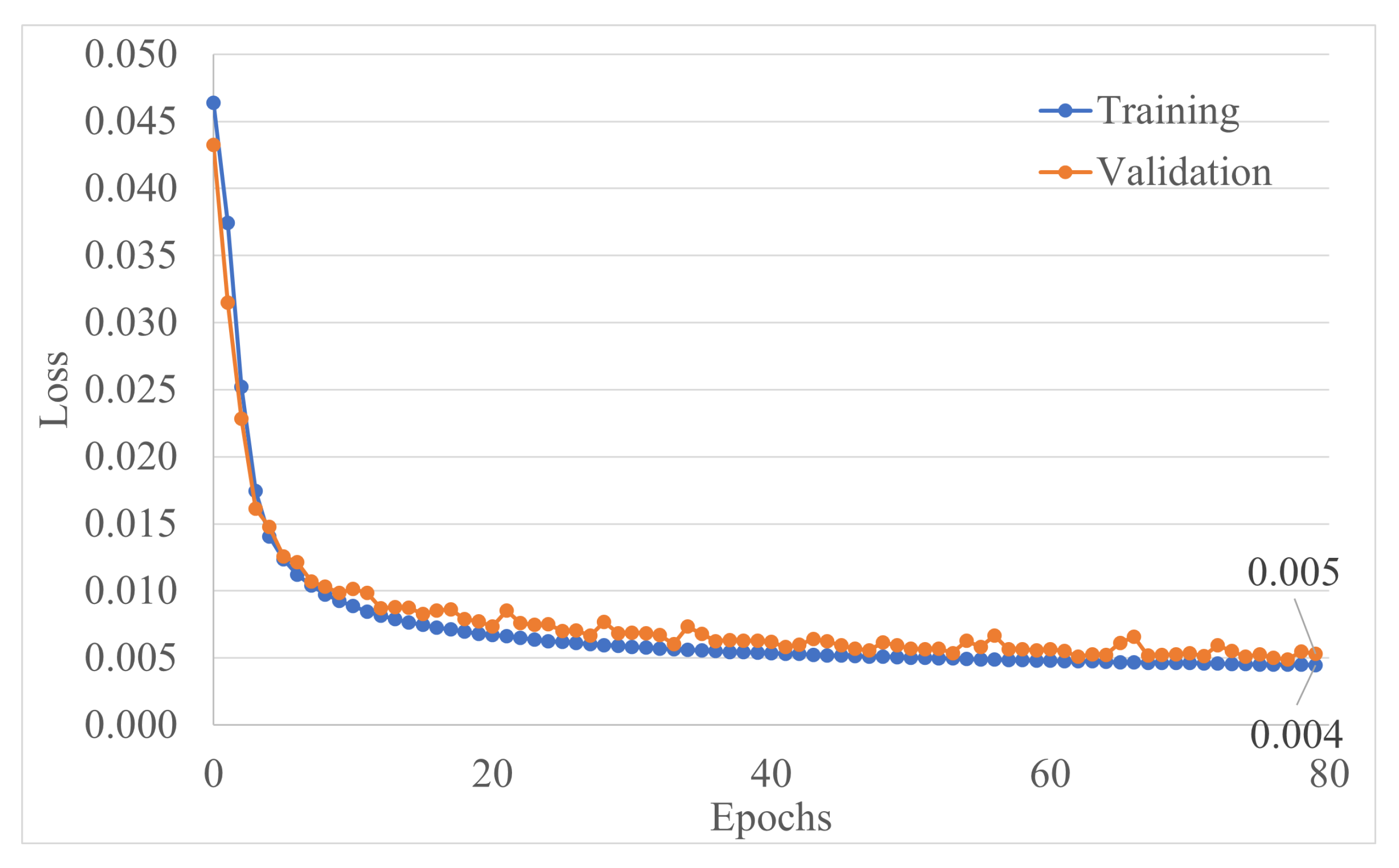
3.3. MLDAR: A Machine Learning-Based Model for Denoising the Ambient Structural Response

In this study, a machine learning-based model is presented that is able to denoise ambient-response recordings collected using instruments with specifications equivalent to those of a low-cost monitoring device (noise density: 22.5 $\mathsf{\mu }\mathrm{g}$/$\sqrt{\mathrm{H}\mathrm{z}}$, MEMS type) used in recent SHM studies [21,26,27,28]. The proposed model is labeled as MLDAR, which stands for Machine Learning-based Denoising of Ambient Response, and is presented graphically in Figure 5. In particular, MLDAR refers to a denoising autoencoder type of neural network whose purpose is to reproduce its inputs’ time histories of ambient structural responses free of noise.

Autoencoders serve as powerful tools for denoising tasks, leveraging their inherent capacity to extract meaningful features from input data while effectively filtering out noise. Comprising both an encoder and a decoder, autoencoders are designed to learn the mapping of noisy input to a lower-dimensional representation, facilitating the subsequent reconstruction of the clean input. The training process involves optimizing the model to minimize the disparity between the reconstructed and pristine inputs, a mechanism that inherently eradicates noise. The denoising prowess of autoencoders arises from their fundamental need to discern between signals and noise. This process highlights the autoencoder’s capability to emphasize salient features within the data, rendering it particularly adept at tasks that demand precision amidst ambient noise. A pertinent application of this capability can be observed in the context of Micro-Electromechanical Systems (MEMs), where autoencoders prove invaluable in enhancing the accuracy of signal extraction in the presence of inherent electronic noise. In essence, autoencoders stand out as versatile tools for noise reduction, excelling in tasks that require the meticulous separation of signals from noise. Their ability to learn intricate patterns in data and prioritize essential features positions them as valuable assets in applications ranging from MEMs to various domains where precision amidst ambient noise is paramount.

The proposed NN model consists of the encoder, the latent space representation, the decoder part, and last but not least, the upscaling part. The input to the proposed model is the noisy ambient response, which can be viewed as a 2D image of size $T\times F$ with two channels, where T represents the time length of the time-history signal, and F denotes the amplitude of acceleration (in $g_s$) at the given time. On the other hand, the output of the model is the corresponding ambient response, clear of any additive noise (e.g., electronic). Its form is also a 2D image with the same size, $T\times F$, as the input.

The signal that precedes the generation of the image takes the form of a time history of acceleration, organized with a consistent timestep. Essentially, it can be envisioned as a one-dimensional matrix encompassing acceleration values, supplemented by a concealed column that incorporates the temporal dimension. This representation is designed to highlight the temporal evolution of the acceleration data, accentuating their dynamic nature in the context of image creation. By structuring the information in this manner, we aim to provide a comprehensive understanding of how acceleration changes over time, offering valuable insights into the intricate process of image generation. The signals throughout this work are not presented as graphs but as images. Therefore, they do not have X- and Y-axes noted in the images themselves. However, they are implied. The X-axis corresponds to samples, and the Y-axis represents acceleration values.

These images are normalized in the range of 0 to 1, a well-known practice for artificial neural networks, depending also on the activation functions adopted. For the needs of the study, a computing system equipped with a standalone NVIDIA Titan RTX graphics card with 24 GB VRAM was used to implement the training part. Relying on the VRAM capabilities, the I/O images’ dimensions were chosen as $512\times 171$ pixels for the input and as $1536\times 512$ pixels for the output. Moreover, in addition to the noise elimination process, an image upscaling process took place with the use of some further levels in the neural network due to input-image compression due to hardware restrictions. The 510 width pixels of input compressed images practically mean that the sampling rate was reduced from 100 Hz to 8.53 Hz. The purpose of the upscaling part is to add the required details to the output signals in order to enable further signal processing techniques, such as the Fast Fourier Transform (FFT), and restore as much of the lost frequency spectrum as possible. After implementing the upscaling process, a sampling rate of 25.6 Hz is restored, meaning that a bandwidth of 12.8 Hz is retained in our signals.

In order to convert images from acceleration values, the following limits were used:

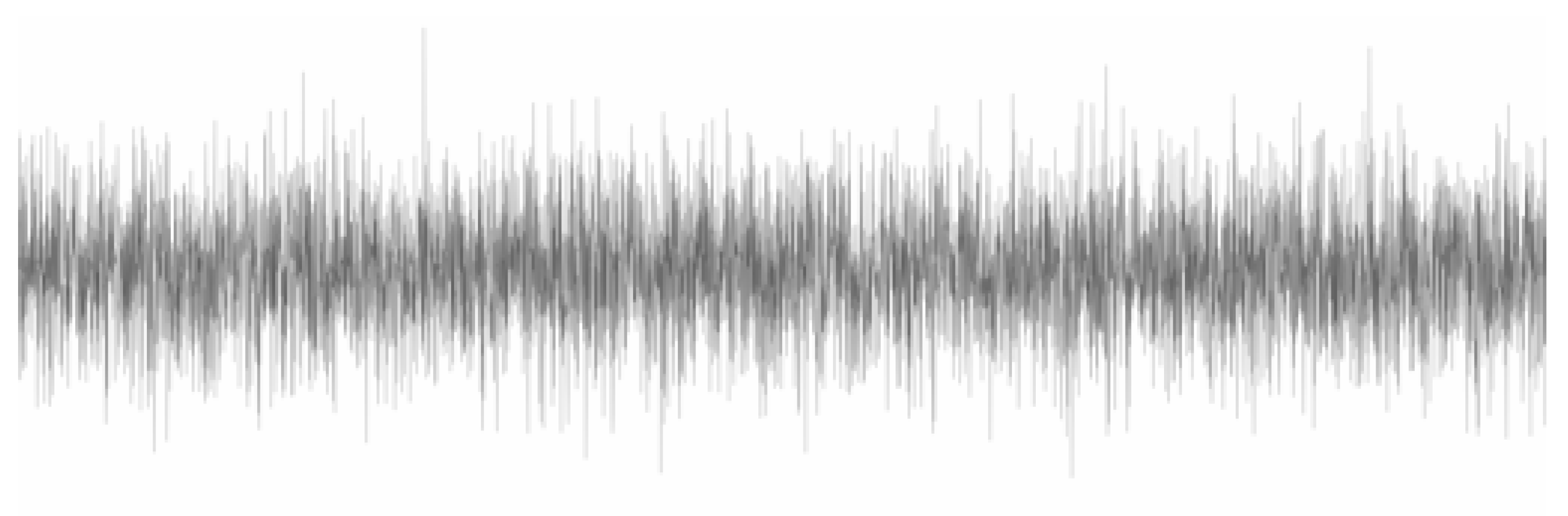
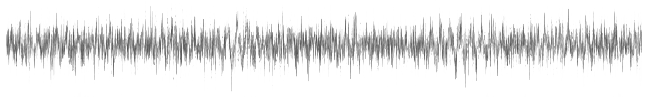
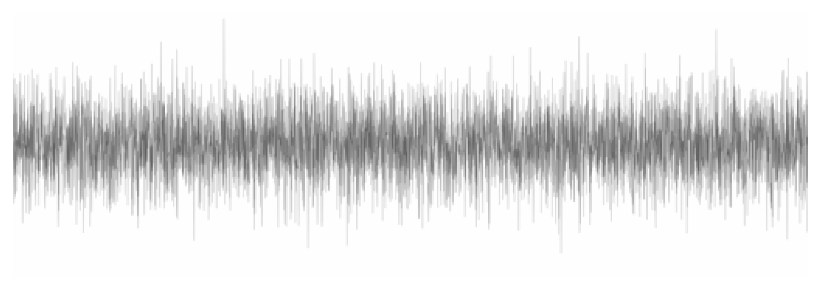
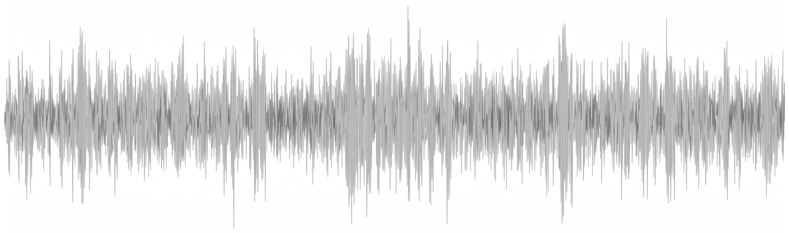
• Input images (noisy response): minimum value of −0.000442 g, maximum value of 0.000437 g;
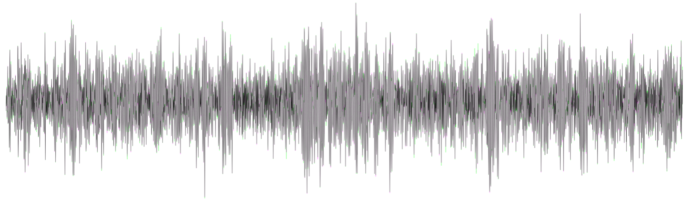
• Output images (no-noise response): minimum value of −0.000074 g, maximum value of 0.000072 g.

The characteristics of the proposed MLDAR model (Figure 5) are the following: the images introduced as input arguments are discretized with $512\times 171$ pixels; therefore, the input format is [171, 512, 1], where 171 refers to the number of pixels along the height of each image, 512 is the number of pixels along the width of each image, and 1 is the value of the monochrome channel (grayscale) of the image. The image is then passed through a 2D convolutional encoder in order to extract the features of major importance. The 2D encoder 

Table 2. Architecture of MLDAR—Part I. “C” indicates a convolutional layer.

	Encoder
	C1 1	C2 1	C3 1	C4 1
Filters:	128	64	64	64
Kernel size:	(2,2)	(2,2)	(2,2)	(2,2)
Dilation:	(1,1)	(2,2)	(4,4)	(6,6)
Stride:	(1,1)	(1,1)	(1,1)	(1,1)
Padding:	Valid	Valid	Valid	Valid

¹ Followed by Batch Normalization, ReLu, and Dropout layers.

consists of four layers of 2D convolution (Conv2D), and ReLu was selected as the proper activation function. Every Conv2D layer is followed by Batch Normalization and Dropout (with a frequency of $25\%$) layers in order to avoid overfitting and so that the network is able to generalize with better accuracy. After implementing the encoding part, two dense layers are used for the latent space representation in order to achieve the desirable compression of the feature values. Feature values were unable to be directly interpreted at the image-pixel input layer; however, it is now possible by means of encoding the latent space representation in a reduced multidimensional space. ReLu is also used as the proper activation function after the small dense layer. Having reshaped the last dense layer to a two-dimensional one, the decoder 

Table 3. Architecture of MLDAR—Part II. ‘C’ indicates a convolutional layer, and “TC” indicates a transposed convolutional layer.

	Decoder				Upscaling
	TC1 1	TC2 1	TC3 1	TC4 1	TC5 1	C5 2
Filters:	64	64	64	128	128	1
Kernel size:	(2,2)	(2,2)	(2,2)	(2,2)	(4,4)	(3,2)
Dilation:	(6,6)	(4,4)	(2,2)	(1,1)	(1,1)	(1,1)
Stride:	(1,1)	(1,1)	(1,1)	(1,1)	(3,3)	(1,1)
Padding:	Valid	Valid	Valid	Valid	Valid	Valid

¹ Followed by ReLu; ² followed by Sigmoid.

is used in order to distance from the feature maps of latent space and return to the composition of the monochrome image. The decoder consists of four levels of Conv2DTranspose, and each of them is complemented by the ReLu activation function. Finally, the upscaling section Table 3 is implemented, which enlarges the image to the desired output size of $1536\times 512$ pixels. Upscaling is implemented at two levels, the Conv2DTranspose and the Conv2D one. The first level relies on a ReLu activation function, while the last one relies on a Sigmoid suppression function, since the output refers to an image with a color value ranging between 0 to 1. Regarding the activation functions, the Sigmoid activation function is characterized by an output range confined within [0,1]. This property proves particularly advantageous when dealing with grayscale images, as their pixel values typically span the range of 0 to 255 (or normalized to 0–1). Sigmoid effectively scales and squashes the output to a probability-like range, aligning well with the characteristics of normalized image data. Conversely, the Rectified Linear Unit (ReLU) activation function introduces crucial nonlinearity to the model, enabling it to discern and learn intricate patterns and representations within the data. Empirically, ReLU has demonstrated robust performance, notably facilitating accelerated convergence during training. In the context of convolutional autoencoders, ReLU is commonly employed in both the encoding and decoding layers. This choice is deliberate, aiming to capture and preserve essential features in the data. The rectification operation inherent in ReLU aids in the learning of hierarchical and spatial features, enhancing the model’s capacity to extract meaningful information from the input.

The loss function chosen corresponds to the mean absolute error between the true label and the prediction (Equation (4)):

$$loss=1/n\sum _{t=1}^n\mid e_t\mid =1/n\sum _{t=1}^n\mid y_{pred}-y_{true}\mid$$

(4)

The batch size was chosen to be six sets of images (input–output). The training took place in 80 epochs. The total number of training parameters was 106,375,947. The Adam optimizer was used on this network with a learning step equal to 0.0001. At the last epoch, the training error was 0.0045, while the prediction error was 0.0053 (in Figure 6, see the history of the training process). The exploration of various model structures, hyperparameters, and training techniques is a crucial aspect of Deep Learning. This iterative process entails systematic testing, evaluation, and subsequent refinement guided by performance metrics. In the initial phase of parameter calibration, our emphasis primarily rested on qualitative comparisons of the results. As the calibration progressed, a transition was made to a more quantitative assessment approach, allowing for a comprehensive analysis of the model’s performance and efficacy. This sequential evolution in our methodology ensures a thorough and balanced evaluation of the experimented variables throughout the experimentation process.

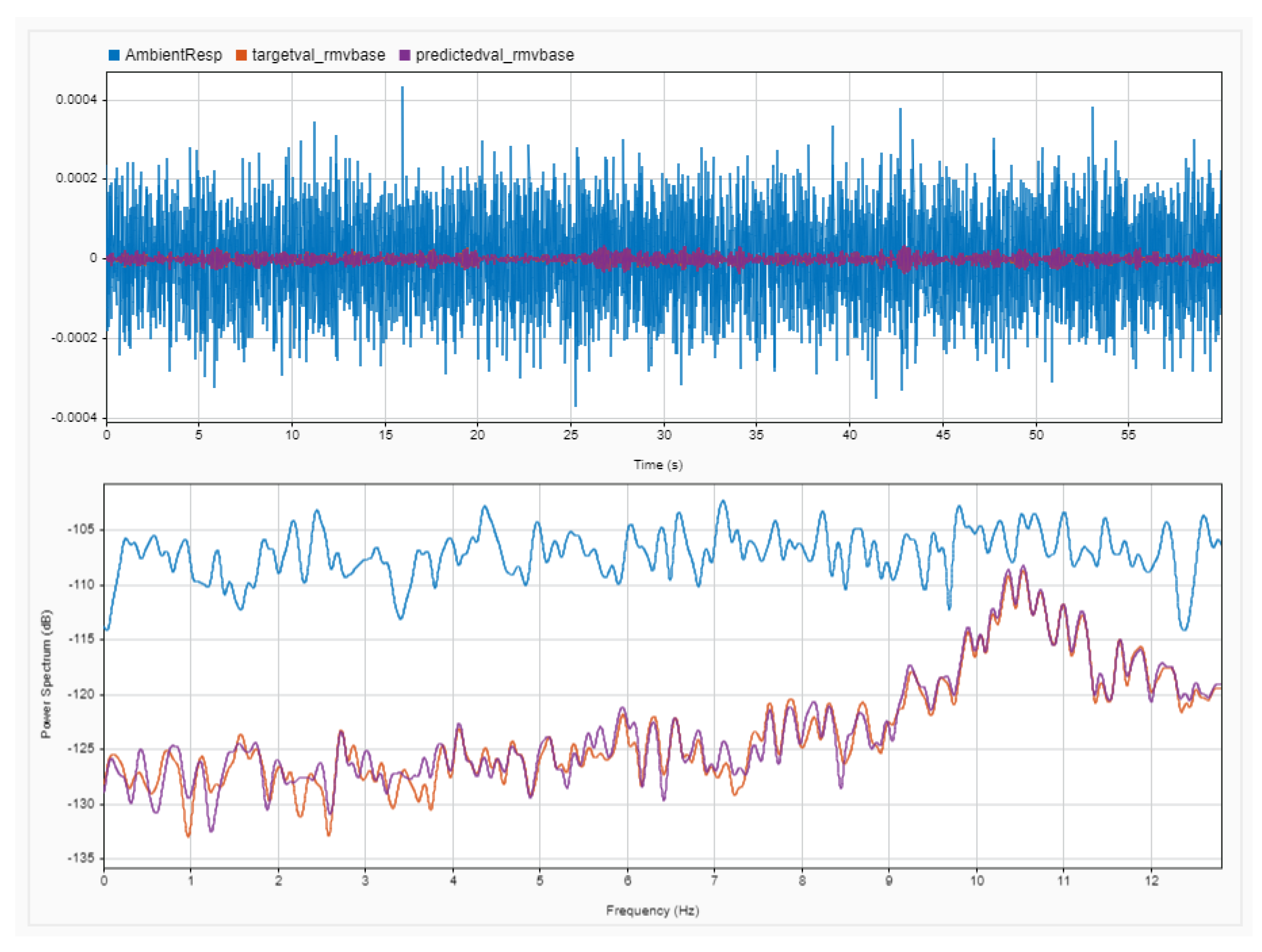
4. Frequency Spectrum Comparison: Qualitative and Quantitative Results

In this part of the study, some of the results obtained in the framework of the investigation are presented. In particular, low-, medium-, and high-frequency signals are randomly selected, aiming to present the efficiency of the proposed MLDAR model for a spectrum of frequency values. Apart from the comparison of the results obtained in terms of images, the frequency content is also compared, the outcome that was the primary goal of the present work.

4.1. Qualitative Comparison: Sample of Low-Frequency Signals

Many mid- to high-rise buildings, bridges, and other flexible structures are usually those showing low-frequency spectral responses, i.e., usually in the range of 1.0 to 3.0 Hz. The dynamic characteristics of these ground-induced structures correspond to a lower acceleration amplitude and a higher displacement amplitude. However, the damping part takes a longer time to diminish the responses to this type of structure. To examine the efficiency of the MLDAR model for such low-frequency cases, a sample denoted as 4_1 was randomly chosen; this sample refers to structural model #4, while the #1 time-window is used to represent the noise. The characteristics of the specific structural model #4 include a frequency value equal to 1 Hz, a one-story structure, and a mass equal to 95% of the reference mass provided in Table 1. The noisy signal can be seen in Figure 7, and the non-noisy one can be found in Figure 8, while the predicted one obtained through the MLDAR model is shown in Figure 9.

In order to make the difference in the magnitude scale (noisy vs. clean signal) more clearly visible, an amplitude comparison between the signal with and without additive noise is provided in Figure 10. This specific sample of noisy signal has values that range in $7.75\times {10}^{-4}$ mg with a standard deviation of $1.02\times {10}^{-4}$ mg. On the other hand, its counterpart, the target non-noisy one, has values that range in $7.27\times {10}^{-5}$ mg with a standard deviation of $9.69\times {10}^{-6}$ mg. As can be seen, the range difference is almost 10 times. To this point, it should be pointed out again that the noisy signal is sampled at 100 Hz, and the non-noisy one, the product and target of the proposed NN, is sampled at 25.6 Hz. The reduction in the sampling rate consequently reduces the level of the total noise. Therefore, calculating the average power of a signal at different sampling rates results in different values. In this case, signal $4\_1$ in the original 100 Hz form has an average power of −79.79 dB, that at 25.6 Hz has an average of −85.81 dB, and the target signal sampled at 25.6 Hz has an average power of −98.80 dB.

Regarding the frequency content of the signals generated by the specific model case, a comparison at the frequency-domain level can be seen in Figure 11. The blue-colored line depicts the noisy signal sampled at 100 Hz, and that was used in the .png format as input in the NN. Orange and violet correspond to the target and predicted non-noisy signals, which show the response of model #4 under ambient vibrations. As can be seen, the 1 Hz frequency is indistinguishable in the ambient vibration measurements due to noise. Even after the averaging of the Fast Fourier Transforms (FTTs) with a 1 min time-window, the 1 Hz frequency cannot be identified. On the other hand, the implementation of the MLDAR model managed to remove the noise from the signal at an acceptable level, where the extraction of the 1 Hz frequency is feasible. As can be seen, the whole frequency band is much lower in the predicted and target signals, showing that the baseline high-level electronic noise has been removed. A comparison in time-history terms can be seen in Figure 12, where differences are colored in green and magenta, and matching regions are in gray.

4.2. Qualitative Comparison: Sample of Medium-Frequency Signal

Many mid-rise buildings, including typical concrete buildings designed based on older building codes, are usually those showing medium-frequency spectral responses, i.e., usually in the range of 3.0 to 6.0 Hz. In order to further examine the efficiency of the MLDAR model, a sample denoted by 631_4 was randomly chosen, belonging to the medium-frequency cases. This sample refers to structural model #631, while the #4 time-window was used to represent the noise. The characteristics of structural model #631 include a frequency value equal to 6 Hz, and similar to the previous case study, it is a one-story structure, and the mass is equal to 80% of the reference mass provided in Table 1. The noisy signal for this specific case can be seen in Figure 13, and the non-noisy one can be found in Figure 14, while the predicted one obtained through the MLDAR model is depicted in Figure 15.

Similar to the low-frequency case, and in order to make the difference in the magnitude scale (noisy vs. clean signal) more clearly visible, an amplitude comparison between the signal with and without additive noise is provided in Figure 16. This specific sample of a noisy signal has values that range in $7.78\times {10}^{-4}$ mg with a standard deviation of $1.03\times {10}^{-4}$ mg. On the other hand, its counterpart, the target non-noisy one, has values that range in $7.20\times {10}^{-5}$ mg with a standard deviation of $1.08\times {10}^{-5}$ mg. As can be seen, the range difference is almost 10 times. For this case, signal $631\_4$ at the 100 Hz sampling rate has an average power of −79.76 dB, that at 25.6 Hz has an average of −85.69 dB, and the target signal sampled at 25.6 Hz has an average power of −95.53 dB.

Regarding the frequency content of the signals generated by the specific model case, a comparison at the frequency-domain level can be seen in Figure 17. The blue-colored line depicts the noisy signal sampled at 100 Hz, and that was used in the .png format as input in the NN. Orange and violet correspond to target and predicted non-noisy signals, which shows the response of model #631 under ambient vibrations. As can be seen, the 6 Hz frequency is indistinguishable in the ambient vibration measurements due to noise. Even after the averaging of the Fast Fourier Transforms (FTTs) with a 1 min time-window, the 6 Hz frequency cannot be identified, as its intensity is much smaller than that of the noise band. On the other hand, the implementation of the MLDAR model managed to remove the noise from the signal at an acceptable level, where the extraction of the 6 Hz frequency is feasible. As can be seen, the whole frequency band is much lower in the predicted and target signals, showing that the baseline high-level electronic noise has been removed. A comparison in time-history terms can be seen in Figure 18, where differences are colored in green and magenta, and matching regions are in gray.

4.3. Qualitative Comparison: Sample of High-Frequency Signal

Low-rise buildings such as those designed and built based on modern design codes or older masonry building structures are usually those showing high-frequency spectral responses, i.e., usually equal to 6.0 Hz or higher. The dynamic characteristics of these ground-induced structures correspond to a higher acceleration amplitude, which, however, is damped at a higher rate of response attenuation. To further examine the efficiency of the proposed MLDAR model for higher-frequency cases, a sample denoted by 1194_7 was randomly chosen. This sample refers to structural model #1194, while the #7 time-window was used to represent the noise. The characteristics of structural model #1194 include a frequency value equal to 10 Hz, a seven-story structure, and a mass equal to 105% of the reference mass provided in Table 1. The noisy signal can be seen in Figure 19, and the non-noisy one can be found in Figure 20, while the predicted one obtained through the MLDAR model is shown in Figure 21.

Similar to the other two cases, for the high-frequency case as well, in order to make the difference in the the magnitude scale (noisy vs. clean signal) more clearly visible, an amplitude comparison between the signal with and without additive noise is provided in Figure 22. This specific sample of noisy signal has values that range in $8.01\times {10}^{-4}$ mg with a standard deviation of $1.04\times {10}^{-4}$ mg. On the other hand, its counterpart, the target non-noisy one, has values that range in $6.94\times {10}^{-5}$ mg with a standard deviation of $1.17\times {10}^{-5}$. As can be seen again, the range difference is almost 10 times. In this case, signal 631_4 at a 100 Hz sampling rate has an average power of −79.70 dB, that at 25.6 Hz has an average of −85.56 dB, and the target signal sampled at 25.6 Hz has an average power of −92.51 dB.

Regarding the frequency content of the signals generated by the specific model case, a comparison at the frequency-domain level can be seen in Figure 23. The blue-colored line depicts the noisy signal sampled at 100 Hz, and that was used in the .png format as input in the NN. Orange and violet correspond to target and predicted non-noisy signals, which shows the response of model #1194 under ambient vibrations. As can be seen, the 10 Hz frequency is indistinguishable in the ambient vibration measurements due to noise. Even after the averaging of the Fast Fourier Transforms (FTTs) with a 1 min time-window, the frequency of interest cannot be identified, as its intensity is much smaller than that of the noise band. On the other hand, the implementation of the MLDAR model managed to remove the noise from the signal at an acceptable level, where the extraction of the target frequency is feasible. As can be seen, the whole frequency band is much lower in the predicted and target signals, showing that the baseline high-level electronic noise has been removed. A comparison in time-history terms can be seen in Figure 24, where differences are colored in green and magenta, and matching regions are in gray.

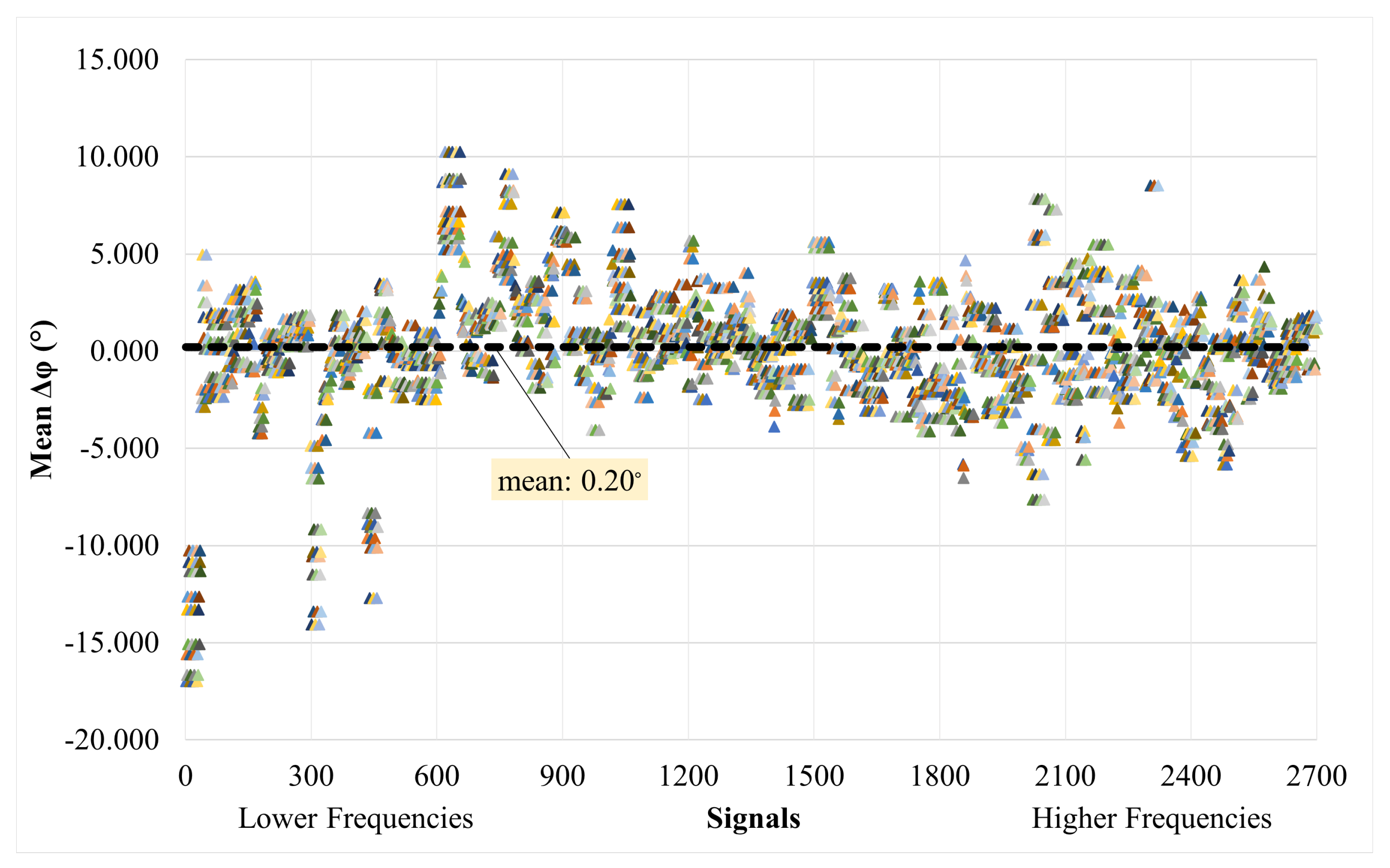
4.4. Quantitative Results: Comparing Frequency Spectra of Prediction and Target for the Whole Dataset through Magnitude-Squared Coherence

Although the denoising process that relies on a Deep Learning model (MLDAR model) concerns acceleration time-history recordings and operates on their image formatting, the main objective of the original problem is the frequency extraction from ambient vibration measurements; thus, the comparison should also be performed on the efficiency of the MLDAR model in extracting eigenfrequencies from the denoised ambient response signals. The first step is to convert the MLDAR image-output dataset into numerical time histories, and then the frequency spectra need to be extracted through the Fast Fourier Transform (FFT) algorithm.

To compare the efficiency of the MLDAR method, a comparison in frequency terms is also performed between predicted and target (original and non-noisy) signals for the validation dataset (i.e., 2700 signals). The validation dataset contains around $25\%$ of the total generated 10,773 signals. Specifically, the magnitude-squared coherence values $C_{xy}\left(f\right)$ (Equation (5)) [29,30,31] are calculated for a specified frequency range between predicted and target signals. Then, the mean value of $C_{xy}\left(f\right)$ for each sample pair of signals is derived. This frequency range depends on the SDOF frequency of interest of each signal and is determined as follows: $f_{SDOF}\pm 0.1$ (Hz). As seen in Figure 25, the minimum mean $C_{xy}\left(f\right)$ value for the whole validation dataset is $91\%$. The average value of the mean $C_{xy}\left(f\right)$ for the whole validation dataset was calculated at $0.98$, with a standard deviation of $0.01$. The standard deviation of $C_{xy}\left(f\right)$ for each sample varies, as shown in Figure 26.

$$C_{xy}\left(f\right)=\frac{{\left|P_{xy}\left(f\right)\right|}^2}{P_{xx}\left(f\right)P_{yy}\left(f\right)}.$$

(5)

where $C_{xy}\left(f\right)$ is the magnitude-squared coherence of the x and y signals, $P_{xx}\left(f\right)$ and $P_{yy}\left(f\right)$ are the power spectral densities of the two signals, and $P_{xy}\left(f\right)$ is the cross-power spectral density of the two signals. $C_{xy}\left(f\right)$ is between 0 and 1.

For purposes of completeness, the phase difference ($\delta \varphi$) between the target and predicted signals in the validation dataset is also presented based on the already-calculated $P_{xy}\left(f\right)$ values, i.e., the cross-power spectral density of the two signals. Similarly, for the same frequency range of each signal, the average of the difference in phase is calculated, and the trend for all signals is summarized in Figure 27. The average value of the mean ($\delta \varphi$) for the whole dataset of signals is calculated as $0.20$ degrees, with a standard deviation of $3.245$. The standard deviation of $\delta \varphi$ for each sample varies, as shown in Figure 28.

Distinctive colors have been introduced in Figure 25 and Figure 27, with the purpose of highlighting the individuality of each graph point, emphasizing their uniqueness within the dataset. The decision to employ varied colors is strategic, as using a uniform color for all points could result in a visually overwhelming amalgamation, resembling a continuous painted area due to the sheer volume of points within the limited horizontal space. By assigning unique colors to each point, we ensure that the values remain discrete and discernible, preventing the potential visual confusion that might arise from a homogeneous color scheme.

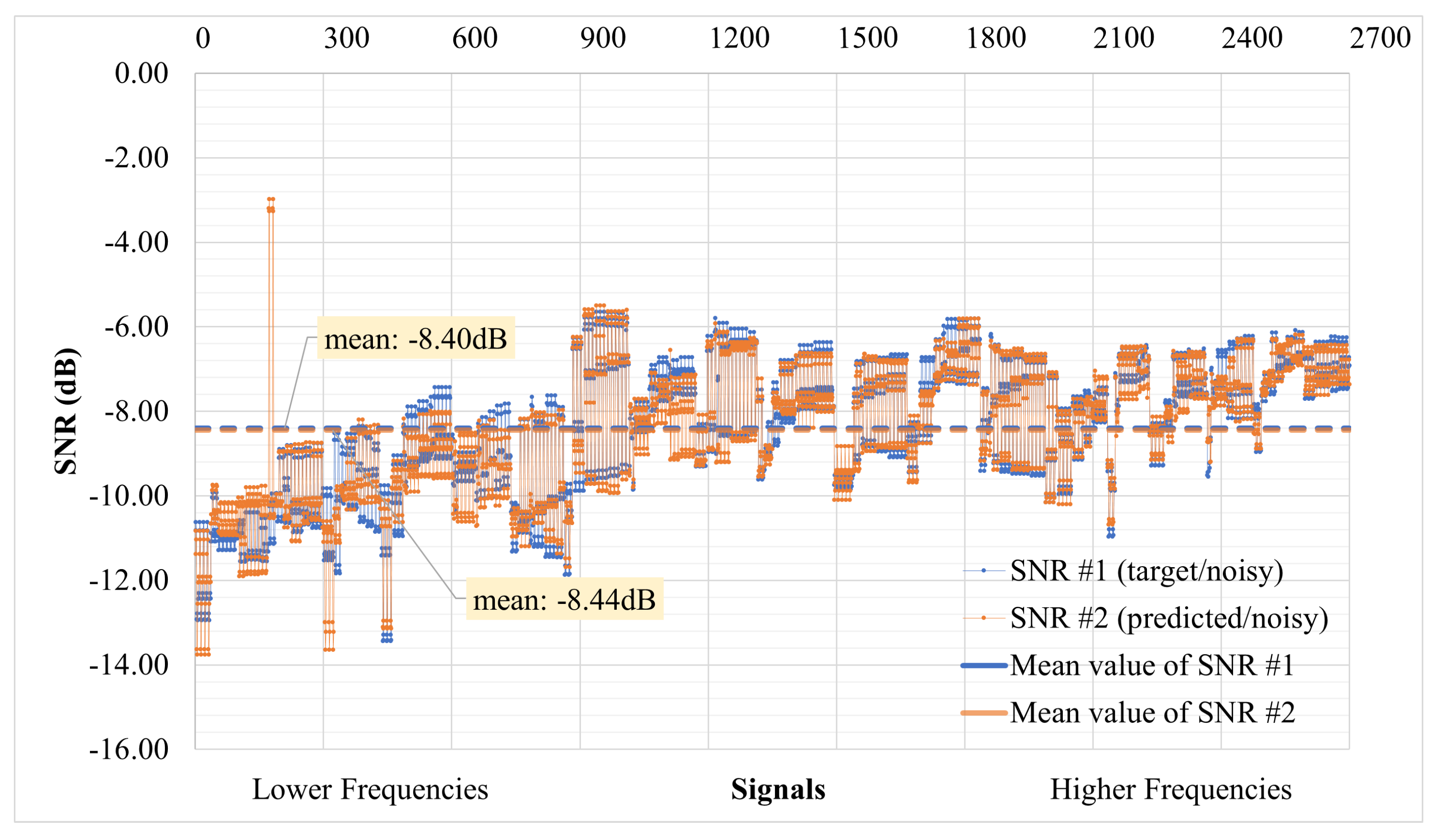
4.5. Quantitative Results: Evaluating Denoising Performance through SNR Levels

Finally, an additional index, the Signal-to-Noise Ratio (SNR) (Equation (6)), was employed to assess the denoising performance. The SNR is a commonly used metric in the fields of science and engineering to compare the level of a desired signal to the level of background noise. It is typically calculated as the ratio of the signal power to the noise power and is often expressed in decibels. An SNR ratio greater than 1:1 (exceeding 0 dB) indicates that the signal strength exceeds that of the noise, thereby signifying a favorable outcome.

$$SNR=\frac{P_{clean}}{P_{noisy}}$$

(6)

The SNR was calculated by taking the average power, denoted by P. The SNR was computed between the noisy and non-noisy signals, specifically between the target and predicted signals. This calculation was performed for the entire validation set, and the corresponding results are presented in Figure 29. SNR#1 refers to the ratio between the target signal and the noisy signal, while SNR#2 represents the ratio between the predicted signal and the noisy signal. The mean value of SNR#1 is found to be −8.40 decibels (dB), indicating a relatively low signal strength compared to the background noise. The median value for SNR#1 is −8.16 dB, suggesting a similar trend in the central tendency of the data. Similarly, the mean of SNR#2 is −8.44 dB, implying a comparable signal–noise relationship for the predicted signal. The median value for SNR#2 is −8.29 dB, reinforcing the observations made from the mean value. These SNR measurements provide quantitative information regarding the relationship between the target or predicted signals and the accompanying noise. The negative dB values indicate that the noise level tends to overshadow the signal strength, highlighting the need for further improvement in denoising techniques to enhance signal clarity.

5. Conclusions

This research proposes the use of a neural network model as a denoiser for ambient vibration measurements, with the primary objective of removing noise while preserving the essential information necessary for subsequent signal manipulation. In this study, signal manipulation refers to the extraction of the dynamic characteristics, such as eigenfrequencies and eigenmodes, of Single-Degree-of-Freedom (SDOF) building models.

In pursuit of denoising various signals, challenges arise after employing a digital sensor or converting an analog sensor output into digital form, leaving limited options for noise reduction. One established approach involves the application of Digital Signal Processing (DSP) techniques, such as digital filtering, moving average filters, and moving median filters. These methods aim to effectively mitigate noise interference. An alternative strategy entails implementing averaging techniques in the frequency domain following the Fourier Transform. This approach proves particularly beneficial in addressing noise issues by exploiting the frequency characteristics of the signals. In the context of analog sensors, the quest for enhanced noise reduction requires a multifaceted approach. This includes the adoption of superior digitization hardware, exemplified by high-quality Analog-to-Digital Converters (ADCs). Furthermore, improvements in shielding for cables and the integration of advanced decoupling transistors contribute significantly to fortifying the system against unwanted noise. Nevertheless, in the specific context of this study, a distinctive choice was made to utilize a Deep Learning architecture for denoising purposes. This decision reflects a departure from traditional techniques, indicating an exploration into the innovative realm of machine learning for noise reduction. By opting for Deep Learning, this study endeavors to leverage the model’s ability to discern complex patterns and extract relevant features, potentially offering a more sophisticated and adaptive solution to the challenges posed by signal noise. This strategic shift aligns with the evolving landscape of signal processing, embracing the promising capabilities of advanced machine learning architectures for effective denoising in diverse sensor applications.

To train and validate the denoiser model, a dataset of response signals was artificially generated based on existing accelerometer noise specifications. Both qualitative and quantitative evaluations demonstrate that the proposed MLDAR model effectively eliminates almost all types of additive noise, including electronic and non-electronic sources, from theoretically noise-free ambient response signals. Despite the significant difference in scale between noisy and noise-free signals, as evident in Figure 10, Figure 16, and Figure 22, the MLDAR model consistently succeeds in removing the noise from the signals. It is worth noting that the MLDAR model produces output signals with a resolution of 12.8 Hz, which is sufficient for most common building structures and civil engineering infrastructures. This limitation is due to the smaller resolution of the input signals compared to the output signals, potentially attributed to hardware capabilities. Nonetheless, the MLDAR model’s upscaling capabilities open avenues for future work, enabling its utilization in versatile and lightweight applications, such as web applications and IoT devices. This makes it possible to combine the denoising model with earthquake building seismic assessment tools and methodologies.

Moreover, the quantitative results of the MLDAR model, as presented in the last paragraph of the numerical investigation section, exhibit its promising performance. The validation dataset shows that the worst performance achieved was a 91% accuracy for only a few cases, while the average score reached 98% (refer to Figure 25). This confirms the successful accomplishment of the primary goal of this study, which is extracting the eigenfrequencies of SDOF building models from noisy signals, a task previously challenging without extending the sampling time or employing statistical signal manipulation techniques [21].

The model was trained using a dataset composed of artificially generated ambient response signals designed to replicate the noise specifications of a MEMS-type accelerometer, specifically the ADXL355 model. These signals were superimposed on the ambient responses of Multi-Degree-of-Freedom (MDOF) building models. The outcomes showcased the efficacy of the MLDAR model in effectively eliminating additive noise from ostensibly noise-free ambient signals. Notably, the model demonstrated this capability despite the substantial scale difference between noisy and non-noisy signals. A constraint observed is the resolution of the output signal images, which restricts the signal’s useful bandwidth to 12.8 Hz, given a sampling rate of 25.6 Hz. Nevertheless, this resolution proves adequate for the majority of building structures and applications in civil engineering. Quantitative assessments affirm the model’s promising performance, with high magnitude-squared coherence scores averaging at 98%, coupled with minimal phase differences of 0.20°. An impressive outcome of the study is the MLDAR model’s capacity to extract fundamental eigenfrequencies from MDOF building models even in the presence of noisy signals, achieving the primary objective without the necessity of extending the sampling time or employing statistical signal manipulation. To further enhance the capabilities of the MLDAR model in future endeavors, several avenues can be explored. Expanded Training Data: Consider retraining the model by incorporating additional data from diverse sensors and ambient vibration field measurements. Real-Time Implementation: Integrate the trained model into a microcontroller or single-board microcomputer/barebone equipped with AI capabilities. This would facilitate the real-time denoising of measurements. Notably, Tensorflow, even in its Tensorflow Lite version, is compatible with a range of low-cost devices (USD 50–150), such as Arduino Nano 33 BLE Sense, Espressif ESP32, Raspberry Pi 4, NVIDIA^® Jetson Nano™, and Coral Dev Board. Versatility Improvement: Explore the possibility of enhancing the model’s versatility in signal denoising tasks, including time-history signals of various natures. This expansion could broaden the applicability of the MLDAR model across a wider spectrum of scenarios.

References

1. Zhang, C.; Mousavi, A.A.; Masri, S.F.; Gholipour, G.; Yan, K.; Li, X. Vibration feature extraction using signal processing techniques for structural health monitoring: A review. Mech. Syst. Signal Process. 2022, 177, 109175. [Google Scholar] [CrossRef]
2. Zinno, R.; Shaffiee Haghshenas, S.; Guido, G.; Vitale, A. Artificial Intelligence and Structural Health Monitoring of Bridges: A Review of the State-of-the-Art. IEEE Access 2022, 10, 88058–88078. [Google Scholar] [CrossRef]
3. Nadkarni, R.R.; Puthuvayi, B. A comprehensive literature review of Multi-Criteria Decision Making methods in heritage buildings. J. Build. Eng. 2020, 32, 101814. [Google Scholar] [CrossRef]
4. Mishra, M. Machine learning techniques for structural health monitoring of heritage buildings: A state-of-the-art review and case studies. J. Cult. Herit. 2021, 47, 227–245. [Google Scholar] [CrossRef]
5. Sony, S.; Dunphy, K.; Sadhu, A.; Capretz, M. A systematic review of convolutional neural network-based structural condition assessment techniques. Eng. Struct. 2021, 226, 111347. [Google Scholar] [CrossRef]
6. Xu, R.; Wu, R.; Ishiwaka, Y.; Vondrick, C.; Zheng, C. Listening to Sounds of Silence for Speech Denoising. arXiv 2020, arXiv:2010.12013. [Google Scholar]
7. Elad, M.; Kawar, B.; Vaksman, G. Image Denoising: The Deep Learning Revolution and Beyond—A Survey Paper. SIAM J. Imaging Sci. 2023, 16, 1594–1654. [Google Scholar] [CrossRef]
8. Izadi, S.; Sutton, D.; Hamarneh, G. Image denoising in the deep learning era. Artif. Intell. Rev. 2023, 56, 5929–5974. [Google Scholar] [CrossRef]
9. Damikoukas, S.; Lagaros, N.D. MLPER: A Machine Learning-Based Prediction Model for Building Earthquake Response Using Ambient Vibration Measurements. Appl. Sci. 2023, 13, 10622. [Google Scholar] [CrossRef]
10. Xiang, P.; Zhang, P.; Zhao, H.; Shao, Z.; Jiang, L. Seismic response prediction of a train-bridge coupled system based on a LSTM neural network. Mech. Based Des. Struct. Mach. 2023, 1–23. [Google Scholar] [CrossRef]
11. Demertzis, K.; Kostinakis, K.; Morfidis, K.; Iliadis, L. An interpretable machine learning method for the prediction of R/C buildings’ seismic response. J. Build. Eng. 2023, 63, 105493. [Google Scholar] [CrossRef]
12. Kohler, M.D.; Hao, S.; Mishra, N.; Govinda, R.; Nigbor, R.L. ShakeNet: A Portable Wireless Sensor Network for Instrumenting Large Civil Structures; US Geological Survey: Reston, VA, USA, 2015.
13. Sabato, A.; Feng, M.Q.; Fukuda, Y.; Carní, D.L.; Fortino, G. A Novel Wireless Accelerometer Board for Measuring Low-Frequency and Low-Amplitude Structural Vibration. IEEE Sens. J. 2016, 16, 2942–2949. [Google Scholar] [CrossRef]
14. Sabato, A.; Niezrecki, C.; Fortino, G. Wireless MEMS-Based Accelerometer Sensor Boards for Structural Vibration Monitoring: A Review. IEEE Sens. J. 2017, 17, 226–235. [Google Scholar] [CrossRef]
15. Zhu, L.; Fu, Y.; Chow, R.; Spencer, B.F.; Park, J.W.; Mechitov, K. Development of a High-Sensitivity Wireless Accelerometer for Structural Health Monitoring. Sensors 2018, 18, 262. [Google Scholar] [CrossRef] [PubMed]
16. Zhou, L.; Yan, G.; Wang, L.; Ou, J. Review of Benchmark Studies and Guidelines for Structural Health Monitoring. Adv. Struct. Eng. 2013, 16, 1187–1206. [Google Scholar] [CrossRef]
17. Yang, Y.; Li, Q.; Yan, B. Specifications and applications of the technical code for monitoring of building and bridge structures in China. Adv. Mech. Eng. 2017, 9, 1687814016684272. [Google Scholar] [CrossRef]
18. Moreu, F.; Li, X.; Li, S.; Zhang, D. Technical Specifications of Structural Health Monitoring for Highway Bridges: New Chinese Structural Health Monitoring Code. Front. Built Environ. 2018, 4, 10. [Google Scholar] [CrossRef]
19. Yang, Y.; Zhang, Y.; Tan, X. Review on Vibration-Based Structural Health Monitoring Techniques and Technical Codes. Symmetry 2021, 13, 1998. [Google Scholar] [CrossRef]
20. Dunand, F.; Gueguen, P.; Bard, P.Y.; Rodgers, J. Comparison of the dynamic parameters extracted from weak, moderate and strong building motion. In Proceedings of the 1st European Conference of Earthquake Engineering and Seismology, Geneva, Switzerland, 3–8 September 2006. [Google Scholar]
21. Damikoukas, S.; Chatzieleftheriou, S.; Lagaros, N.D. First Level Pre- and Post-Earthquake Building Seismic Assessment Protocol Based on Dynamic Characteristics Extracted In Situ. Infrastructures 2022, 7, 115. [Google Scholar] [CrossRef]
22. ADINA, version: 9.2.1; ADINA R&D Inc.: Watertown, MA, USA, 2016. Available online: http://www.adina.com/(accessed on 19 September 2022).
23. FEMA. Hazus—MH 2.1: Technical Manual; Department of Homeland Security, Federal Emergency Management Agency, Mitigation Division: Washington, DC, USA, 2013. [Google Scholar]
24. MATLAB, version 9.11.0 (R2021b); The MathWorks Inc.: Natick, MA, USA, 2021.
25. LeCun, Y.; Boser, B.; Denker, J.S.; Henderson, D.; Howard, R.E.; Hubbard, W.; Jackel, L.D. Backpropagation Applied to Handwritten Zip Code Recognition. Neural Comput. 1989, 1, 541–551. [Google Scholar] [CrossRef]
26. Shabani, A.; Feyzabadi, M.; Kioumarsi, M. Model updating of a masonry tower based on operational modal analysis: The role of soil-structure interaction. Case Stud. Constr. Mater. 2022, 16, e00957. [Google Scholar] [CrossRef]
27. Unquake. Unquake Accelerograph-Accelerometer Specifications. Available online: https://unquake.co (accessed on 19 September 2022).
28. Chatzieleftheriou, S.; Damikoukas, S. Optimal Sensor Installation to Extract the Mode Shapes of a Building—Rotational DOFs, Torsional Modes and Spurious Modes Detection. Technical Report. Unquake (Structures & Sensors P.C.). 2021. Available online: https://www.researchgate.net/institution/Unquake/post/6130bc2ca1abfe50c1559a26_Download_White_Paper_Optimal_sensor_installation_to_extract_the_mode_shapes_of_a_building-Rotational_DOFs_torsional_modes_and_spurious_modes_detection (accessed on 19 September 2022).
29. Welch, P. The use of fast Fourier transform for the estimation of power spectra: A method based on time averaging over short, modified periodograms. IEEE Trans. Audio Electroacoust. 1967, 15, 70–73. [Google Scholar] [CrossRef]
30. Rabiner, L.R.; Gold, B. Theory and Application of Digital Signal Processing; Prentice-Hall: Englewood Cliffs, NJ, USA, 1975. [Google Scholar]
31. Kay, S. Spectral Estimation. In Advanced Topics in Signal Processing; Prentice-Hall, Inc.: Englewood Cliffs, NJ, USA, 1987; pp. 58–122. [Google Scholar]
Figure 1. Typical building model in ADINA on which assumptions-table is referring to.
Computation 12 00031 g001
Figure 2. Bilinear capacity curve of all structural members.
Computation 12 00031 g002
Figure 3. A 2D CNN channel.
Computation 12 00031 g003
Figure 4. The general structure of an autoencoder, mapping an input x to an output (called reconstruction) r through an internal representation or code h. The autoencoder has two components: the encoder f (mapping x to h) and the decoder g (mapping h to r).
Computation 12 00031 g004
Figure 5. The MLDAR neural network model.
Computation 12 00031 g005
Figure 6. Training and validation loss function values over 80 epochs.
Computation 12 00031 g006
Figure 7. The noisy low-frequency signal (signal 4_1).
Computation 12 00031 g007
Figure 8. The low-frequency signal without noise [Target] (signal 4_1).
Computation 12 00031 g008
Figure 9. The denoised low-frequency signal through the MLDAR model [Prediction] (signal 4_1).
Computation 12 00031 g009
Figure 10. Low-frequency case: scale comparison between noisy signal and non-noisy (cleaned–predicted).
Computation 12 00031 g010
Figure 11. Low-frequency case: comparison of frequency content between response to ambient noise (blue), target signal (orange), and predicted signal (violet)—frequency of 1.0 Hz.
Computation 12 00031 g011
Figure 12. Low-frequency case: comparison of frequency content between target signal (orange) and prediction (light blue)—frequency of 1.0 Hz.
Computation 12 00031 g012
Figure 13. The noisy medium-frequency signal (signal 631_4).
Computation 12 00031 g013
Figure 14. The medium-frequency signal without noise [Target] (signal 631_4).
Computation 12 00031 g014
Figure 15. The denoised medium-frequency signal through the MLDAR model [Prediction] (signal 631_4).
Computation 12 00031 g015
Figure 16. Medium-frequency case: scale comparison between noisy signal and non-noisy (cleaned–predicted).
Computation 12 00031 g016
Figure 17. Medium-frequency case: comparison of frequency content between response to ambient noise (blue), target signal (orange), and predicted signal (violet)—frequency of 6.0 Hz.
Computation 12 00031 g017
Figure 18. Medium-frequency case: Comparison of frequency content between target and predicted non-electronically noisy signals. Differences are highlighted by orange and magenta colors, and matching regions are in gray—frequency of 6.0 Hz.
Computation 12 00031 g018
Figure 19. The noisy high-frequency signal (signal 1194_7).
Computation 12 00031 g019
Figure 20. The high-frequency signal without noise [Target] (signal 1194_7).
Computation 12 00031 g020
Figure 21. The denoised high-frequency signal through the MLDAR model [Prediction] (signal 1194_7).
Computation 12 00031 g021
Figure 22. High-frequency case: scale comparison between noisy signal and non-noisy (cleaned–predicted).
Computation 12 00031 g022
Figure 23. High-frequency case: comparison of frequency content between response to ambient noise (blue), target signal (orange), and predicted signal (violet)—frequency of 10.0 Hz.
Computation 12 00031 g023
Figure 24. High-frequency case: Comparison between target and predicted non-electronically noisy signals. Differences are highlighted by orange and magenta colors, and matching regions are in gray—frequency of 10.0 Hz.
Computation 12 00031 g024
Figure 25. Mean magnitude-squared coherence C x y ( f ) for whole validation dataset between target and predicted signals.
Computation 12 00031 g025
Figure 26. Standard deviation of magnitude-squared coherence C x y ( f ) for whole validation dataset between target and predicted signals.
Computation 12 00031 g026
Figure 27. Mean phase difference ( δ ϕ ) for whole validation dataset between target and predicted signals.
Computation 12 00031 g027
Figure 28. Standard deviation of phase difference ( δ ϕ ) for whole validation dataset between target and predicted signals.
Computation 12 00031 g028
Figure 29. Signal-to-Noise Ratio (SNR) for whole validation dataset between target and predicted signals.
Computation 12 00031 g029