Abstract
Fused-Deposition Modeling (FDM) is a commonly used 3D printing method for rapid prototyping and the fabrication of plastic components. The history of temperature variation during the FDM process plays a crucial role in the degree of bonding between layers. This study presents research on the thermal analysis of the 3D printing process using a developed simulation code. The code employs numerical discretization methods with an implicit scheme and an effective heat transfer coefficient for cooling. The computational model is validated by comparing the results with analytical solutions, demonstrating an agreement of more than 99%. The code is then utilized to perform thermal analyses for the 3D printing process. Interlayer and intralayer reheating effects, sensitivity to printing parameters, and realistic printing patterns are investigated. It is shown that concentric and zigzag paths yield similar peaks at different time intervals. Nodal temperatures can fall below the glass transition temperature (Tg) during the printing process, especially at the outer nodes of the domain and under conditions where the cooling period is longer and the printed volume per unit time is smaller. The article suggests future work to calculate welding time at different conditions and locations for the estimation of the degree of bonding.
1. Introduction
Additive manufacturing technologies are undergoing rapid advancements in the contemporary landscape. Among the diverse array of three-dimensional (3D) printers designed for various materials, Fused-Deposition Modeling (FDM) stands out as a widespread choice for prototyping and the fabrication of plastic components. In this innovative process, plastic filaments undergo controlled melting via a dynamic nozzle, strategically deposited layer by layer onto a surface to form a predetermined shape. This layering technique is instrumental in crafting preset geometry definitions with precision and efficiency. When compared to manufacturing technologies such as CNC (Computer Numerical Control) machining, it is seen that the FDM method is a production method that consumes significantly less energy and generates less waste [1]. On the other hand, quality issues are observed in parts produced via FDM [2]. The main reason for quality problems is the variations in interlayer bond strength (polymer diffusion) depending on time-dependent changes in temperature [3]. To solve quality problems, the effect of parameters related to both polymer diffusion and heat transfer, such as extrusion temperature, layer thickness, heating–cooling profile, production speed, adhesion surface width, and substrate surface temperature, on quality should be examined.
The layers, which are stacked on top of each other in accordance with the pre-defined geometry of the three-dimensional part to be produced, are held together by polymer bonds. The polymer structures in the plastic layers pass from one layer to the other by diffusion, which provides adhesion [4]. The durability of the constructed part depends on the completion of the polymer diffusion at the layer-to-layer interface [5]. The ratio of the strength () of the part produced by FDM to the strength of the bulk material () gives the degree of bonding (Dh) [3]:
According to Edwards [6], a polymer resides in a virtual tube where it does not interact with other polymers around it. The time required for the polymer to come out of this tube is called the reptation time (τrep). Materials that exceed the reptation period are considered to form the bonds that provide the highest strength. According to Edward’s Tube Theory, the shorter the reptation time, the faster the binding occurs.
In polymer–polymer interlayers that do not reach the reptation time, the durability () becomes lower. The welding time () of the parts that cannot reach the reptation time is proportional to ()1/4 [7].
On the other hand, the temperature in the interlayers and the history of temperature variation affect the . For example, while the printing process takes place at the upper layers, heat diffusion from the upper layers to the lower ones can raise the temperature on the below layers above the glass transition temperature (Tg), which will affect the bonding there. Hence, it is important to monitor the temperature of each layer during the whole printing process. It should be examined by which layers and at what time intervals interlayer temperatures are below or above Tg. It is predicted that the layer with the shortest binding time will have the weakest point. In an experimental study [8], it was observed that the strength of the upper layers was higher in the production scenario tested. A comprehensive heat transfer analysis model is needed to predict which layer is the weakest under different conditions and production parameters.
There are computational, experimental, and analytical studies in the literature on thermal analysis of the FDM process. In a comprehensive literature survey spanning multiple studies, diverse approaches have been employed to analyze and understand the time-dependent thermal response of printed material during additive manufacturing processes.
Yang et al. focused on the analytical and experimental investigation of polymeric materials, specifically PEEK and PEKK, under non-isothermal conditions [3]. The study developed a degree of bonding (Dh) formula analytically and validated it through experiments, emphasizing that time-dependent temperature variations have a significant impact on the degree of bonding.
Sun et al. shifted the focus to ABS, employing both analytical and experimental methods [9]. It measured the time-dependent variations in temperature of the first layer with an embedded thermocouple in the base plate during 15-layer and 30-layer production, noting that in the 30-layer production, the temperature on the bed surface fell below the glass transition temperature.
Another study in the literature performed experiments concentrating on ABS and utilizing infrared (IR) temperature measurements during FDM [10]. In this study, Seppala et al. specifically examined the lower and upper surface temperatures of the top layer, highlighting the effectiveness of IR technology for temperature measurements at various layer heights. Based on the infrared measurements conducted on the part geometry and extrusion conditions under investigation, it was observed that the temperature of the printed layer decreases rapidly. Only a minimal amount of heat was transferred to the first sublayer, and the second sublayer never attains the glass transition temperature.
Coogan et al. contributed to the exploration of ABS through experimental means, investigating the effects of extrusion temperature, bed temperature, speed, distance from the bed, layer thickness, and fiber width on strength [8]. Notably, the study observed higher strength in the upper layers compared to those closer to the bed. It is recommended by the authors that time-dependent temperature behavior at the interface between consecutive layers should be assessed in future works. In their following article, Coogan et al. employed a computational approach adopted for ABS, utilizing 1D heat transfer calculations to model the top two layers [11]. And two-dimensional computational analysis is advised for the further enhancement of numerical modeling.
Bartolai et al. maintained an experimental focus on ABS, incorporating infrared (IR) temperature measurements [5]. The study leveraged the temperature history to estimate the strength of the printed parts, providing a nuanced exploration of the interplay between temperature dynamics and mechanical performance. However, since this estimation is based on a single interlayer interface, other interfaces should be analyzed to obtain a comparison between the interlayers.
A hybrid computational and experimental approach was taken for TPU-ABS by Yin et al., with two different materials produced side by side using FDM [12]. The study revealed that the strength of the part increased with an elevation in the bed temperature.
Basgul et al. performed an analysis of the production of Polyether Ether Ketone (PEEK) through the fused filament fabrication (FFF) method [13]. A one-dimensional (1D) Heat Transfer Model (HTM) is developed in Matlab to calculate layer and interlayer temperatures. In this model, the 1D finite difference method is employed with an explicit discretization scheme. The natural convection correlation is calculated as h = 17.5 W/m2-K to define convection boundary conditions for cooling. Apart from a numerical study, thermal videos are recorded via experimentation using an infrared camera, and these thermal images are subsequently processed to obtain time-dependent layer temperature profiles for FFF PEEK prints. Particularly, discrepancies between experimental and numerical data are observed, especially in the lower layers. This result points out the necessity of more accurate numerical modeling, which is required to capture accurate temperature values.
An analysis conducted by Zhang et al. presented a numerical investigation of the influence of process conditions on temperature variations in FDM using PLA [14]. The trajectory of the extrusion is defined as zigzag patterns. The researchers developed a 3D finite difference code with an explicit discretization scheme, defining a constant air temperature as a boundary condition on surfaces. In another study in the literature, Zhang et al.’s computation model is compared to the experimental results that show underprediction of temperature values at the upper layers [15].
A three-dimensional computational model has been employed to analyze the transient heat transfer problem using a commercial code called ANSYS by Khanafer et al. [16]. The printing trajectory is applied from left to right for each layer, with no production in the backward direction along the depth axis. An additional dwell (cooling) time is defined to account for 3D effects. However, it is important to note that since the numerical modeling in the third dimension constitutes unit depth, this approach disregards intralayer conduction in the z direction and thermal peaks due to this intralayer conduction.
Ramos et al. performed a numerical study using the Ansys Mechanical APDL software to analyze heat transfer during fused filament fabrication [17]. The numerical analyses are validated with the temperature values measured using three K-type thermocouples located at different layers by pausing the printing process. It is observed in the comparative plots that numerical temperatures and cooling rates differ significantly from the experimental ones. This study utilizes an adapting mesh to perform calculations in a more efficient way. Multiple controlling parameters are defined to coarsen the mesh at symmetrical locations in the lower parts of the domain. However, for the analysis of complex geometries with no symmetry, the mesh coarsening process has the potential to add extra computational load.
Mosleh et al. performed research on the thermal dynamics occurring during the initial layer deposition in 3D printing, specifically focusing on the numerical and experimental investigation of ABS deposition [18]. The examination employs both infrared thermometry and COMSOL Multiphysics software. However, the numerical analyses performed are restricted to a 2D framework, with a computed numerical relative error of 7% when compared to infrared measurements. A limitation of the study lies in the absence of considerations for 3D printing pattern effects and the intricacies of heat diffusion in three dimensions. Additionally, the study’s scope is confined to the analysis of a single layer, precluding the exploration of interlayer and intralayer effects.
These collective studies contribute rich insights into the thermal aspects of various materials, offering a holistic understanding of the necessity of time-dependent 3D thermal modeling of additive manufacturing processes and paving the way for advancements in optimizing parameters for enhanced material performance. However, thermal analyses play a crucial role in the prediction of temperature history at locations where temperature cannot be measured with experimental methodologies such as infrared imaging. In order to obtain accurate temperature predictions, a study should be performed that models the printing process in the depth direction via 3D heat transfer analysis to be able to accurately capture thermal behavior in 3D printing with an accurate computational model. Commercial computer-aided engineering tools need interventions with extra coding to control air-to-material boundaries and related boundary conditions (e.g., conduction, convection) that dynamically change throughout the printing process. Hence, a three-dimensional heat transfer analysis code with a finite difference method and an implicit discretization scheme has been developed with the Fortran programming language from scratch to be able to control and perform thermal analyses comprehensively and accurately.
2. Mathematical Modeling and Conditions
The objective of this study is to analyze temperature variations in the 3D printing process through the utilization of a purpose-built in-house thermal analysis code. The 3D nature of the printing process and the dynamic evolution of boundaries during the procedure render the application of existing commercial heat transfer simulation software more challenging. In order to accommodate different printing parameters flexibly and establish a basis for subsequent polymer diffusion calculations influenced by temperature history, an in-house code has been developed for simulating the 3D printing process using computational methods. The three-dimensional transient heat diffusion equation is discretized with an implicit scheme to achieve convergence independent of mesh size. A mesh-size study is undertaken to obtain accurate results as a consequence of the simulations conducted with the code. The code’s validation is carried out through the utilization of an analytical approach, as described in the following section in detail.
2.1. Governing Equations and Discretization Scheme
The general form of the equation expressing the time-varying diffusion of heat in a solid is as follows:
Equation (3) was discretized according to the template shown in Figure 1 according to the finite difference method [19]. In discretization, center differences in x, y, and z directions and back-differences in time are employed. The discretized equation is given in Equation (4). Local definitions of the i,j,k indices are depicted in Figure 1. Heat generation term in Equation (2), q/k, is assumed to be zero.
where T is temperature, t is time, p is the index showing previous time step, p + 1 is the index showing current time step, is distance between nodes on x direction, is distance between nodes on y direction, is distance between nodes on z direction, and is thermal diffusivity described as .
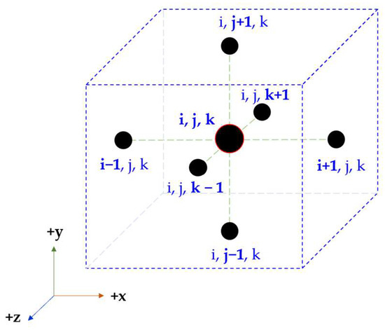
Figure 1.
Schematic representation of i,j,k indices.
Based on the discretization parameters, the number of nodes in the domain is a definite number. Equation (3) is valid for each nodal point in the computational domain, and the total number of equations is equal to the total number of nodes. With an implicit discretization scheme, these equations should be expressed and solved in a matrix form, . Here, A is the coefficient matrix, and the T vector includes unknown temperatures, that is, T(i,j,k) values at p + 1. The terms (coefficients) in the matrix are named with a(i,j,k) indices in the coefficient matrix. The b vector on the right includes known values (right-hand side, RHS) of the equation, i.e., temperatures at the previous time step (p) and known boundary conditions.
When there is a convection boundary condition at the boundaries, Newton’s law of cooling is utilized as a boundary condition at the nodes that are exposed to air. In order to consider the heat transfer by radiation, an effective heat transfer coefficient (heffective) is defined. This coefficient is the sum of convective and radiative heat transfer coefficients, which is calculated as follows:
where is the temperature of the surrounding environment, ϵ is emissivity, and σ is Stefan-Boltzmann constant. Figure 2 shows a schematic representation of the computational domain and corresponding boundary temperatures in 3D.
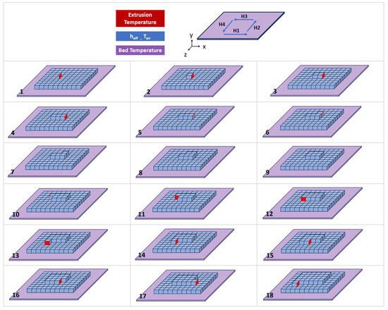
Figure 2.
Schematic representation of trajectory and dynamic boundary conditions updated with trajectory, and definition of H1, H2, H3, and H4 directions.
Equation (3) is rearranged to obtain a leaner form depicting constituent physics grouped in terms. In order to simplify Equation (4), below Biot and Fourier numbers are used:
After some algebraic manipulations, the concluding equation is as follows:
In the coefficient matrix, it is possible to group the coefficients of the according to physics. These terms and the physical phenomenon they represent can be summarized as follows:
- Conduction in x, y, and z directions.
- Convection and radiation () in x, y, and z directions.
- Temperature change in time.
The coefficients represented in group II are zero for the inner (solid) nodes. However, at the boundaries subject to air, the corresponding terms in exposed directions are not zero. In the light of this information, the formula can be generalized for the boundary and inner regions. For this, it must be known whether the adjacent node is in air or in the printed solid area. In order to dynamically update the equation per its air or solid state, the “fill” state function is defined as follows:
Since there are six points in the neighborhood of a single node, the calculation should be made by checking the state of these six neighboring points. Parameters defined with the state control at each neighboring point are provided in Table 1.

Table 1.
Functions representing the boundary effect from nodes adjacent to the node (i, j, k).
With the sum of coefficients given in Table 1 defined as “BC”, Equation (7) simplifies to Equation (9).
In addition, a state definition should be made for conductive terms in the coefficient matrix. When the node is filled with material, there should be conduction, otherwise the corresponding coefficient should be adjusted to zero. After some algebraic re-arrangements, coefficients that belong to group I are obtained as given in Table 2. The known values grouped in the b vector are also provided.
Table 2.
Functions representing the conduction effect from nodes adjacent to the node (i,j,k).
2.2. Definition of Printing Path
The path defined in the scope of this study is a spiral from left to right, inwards to outwards. Note that the –z direction is the depth of the printed part.
In the simulation, a new node at a temperature of extrusion is progressed along the path direction defined in Figure 2 to mimic the printing process. The fill function of this new node is set to 1; hence, it is filled with polymeric material.
2.3. Nominal Production Parameters and Material Properties
- Extrusion temperature (Text) is equal to 210 °C.
- Bed temperature (Tbed) is 60 °C.
- The air temperature is assumed to be 20 °C.
- The nominal effective heat transfer coefficient (heff) is 50 W/m2-K.
- Production speed is 60 mm/s.
- Density of PLA: 1240 kg/m3 [20].
- Specific heat (cp) of PLA: 1800 J/kg-K [21].
- Conductivity (k) of PLA: 0.13 W/m-K [21].
2.4. Modeled System and Solution Parameters (Nominal Case)
- X direction: The width of the part is 8 mm, divided into 24 parts (Δx = 0.333 mm).
- Y direction: The part is printed in 20 layers. The layer thickness is taken as 0.3 mm. The total height is 6 mm (Δy = layer thickness = 0.3 mm).
- Z direction: The depth of the part is 4 mm, divided into 12 parts (Δz = 0.333 mm)
- Time step: The algorithm is designed to advance 1 node in each time step. The time step size is calculated as Δt = Δx/speed = 0.005556 s.
3. Validation of the Methodology
3.1. Definition of the Benchmark Case
A representative geometry is specified for conducting computational and analytical calculations to validate the results. The dimensions of the geometry are defined with total lengths along the x, y, and z directions as 8 mm, 12 mm, and 4 mm, respectively. Note that the total height of this benchmark case is set to 12 mm, which corresponds to 40 layers in a nominal case, while considering future work that might need more layers.
The initial condition is characterized by a uniform temperature pattern set at 210 °C. The heat transfer coefficient is established at 50 W/m2-K, and the air temperature is maintained at 20 °C. It is noteworthy that the boundaries of this geometry remain constant over time, ensuring the applicability of analytical formulations.
3.2. Analytical Solution
The developed in-house code is validated in comparison to the analytical transient heat transfer formulation in plane wall geometry provided in [22]. The general form of this equation is the solution of the heat diffusion equation with the help of Fourier Series expansion [22]:
Eigenvalues are positive roots of the equation below [22]:
Note that this solution is valid for 1D temperature distribution on the x-axis inside a plane wall (slab) with an infinite dimension on other directions. A multidimensional solution can be obtained with the production of one-dimensional results that are separately calculated on x, y, and z dimensions in regard to proper orthogonal decomposition method.
A 10-term approximation is employed to estimate the analytical results since one-term approximation does not provide accurate results for Fo > 2 [22]. A 3D analytical solution for a rectangular prism can be obtained using the below equation:
At the center of the geometry, , , and are equal to zero. With cos(0) = 1, the above equation reduces to the following:
First 10 root of the Equations (11) and (12) and corresponding coefficient values are given in Table 3 [22].
Table 3.
First 10 roots and coefficients of Equations (11) and (12) [22].
By varying the time, Equation (16) yields temporal temperatures. Hence, the analytical solution of the transient temperature change at the center of the geometry is obtained. Analytical results are utilized to validate the in-house code described in Section 3.4.
3.3. Mesh Study
In a computational study, the accuracy level of the solution is unsatisfactory with large mesh sizes (i.e., large Δx, Δy, and Δz values, which means coarse mesh in the computational domain). Therefore, it is crucial to see whether the mesh size is acceptable for both accuracy and computation time aspects. A smaller mesh size increases the number of nodes in the domain, and it starts to require more computing power and runtime. The solution becomes adequately accurate when it converges to a certain pattern that is independent of the mesh structure. In order to define the minimum number of nodes required to obtain an adequately accurate temperature distribution with a computational model, a mesh study should be performed (Figure 3). In the legend of Figure 3, the number of meshes on the x, y, and z axes is given, respectively.
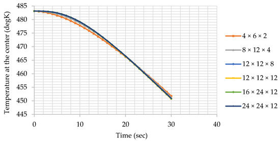
Figure 3.
Temperature results obtained at the center of the benchmark geometry with different mesh sizes in x, y, and z directions.
Relative change between results reaches to the order of 0.01% for Mesh 6, as given in Table 4. Therefore, 24 × 24 × 12 divisions on the axes provide results that are almost independent of the discretization. This structure corresponds to Δx = 0.333 mm, Δy = 0.5 mm, and Δz = 0.333 mm.
Table 4.
Mesh study results and relative changes (%).
3.4. Validation
Furthermore, a comparative analysis is performed to observe the difference between computational and analytical results. The temperature change with respect to time is depicted in Figure 4 for this purpose.
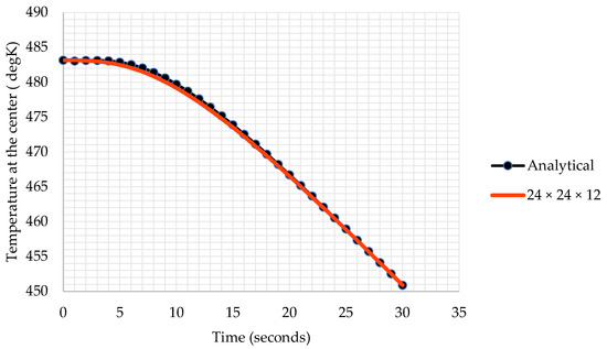
Figure 4.
Comparison between the computational and the analytical solutions.
The disparity between computational and analytical results is minimal, with a maximum difference of only 0.12%. This negligible distinction indicates that the computational tool is well suited for the analysis of the 3D printing process. It is important to highlight that, for an accurate modeling of the 3D printing process, the spatial increment Δy needs to be on the scale of the layer thickness, typically within the order of microns. To achieve this precision, a finer mesh is employed in the y direction to effectively capture the nuances of the layer thickness.
4. Results
In this section, the outcomes of the numerical investigation into temperature variations during the 3D printing process are presented. The analysis of temperature changes was conducted through the developed and validated solver, as described in previous sections. The results were derived from numerical experiments by using this code with the geometry and parameters defined in Section 2.2 and Section 2.3 (nominal case).
A detailed perspective on the temperature dynamics inherent to 3D printing is offered. The patterns and fluctuations in temperature are highlighted, providing a foundational understanding for further discussion.
4.1. Temperature Contour Plots
The heating and cooling patterns are clearly observed in three dimensions, as illustrated in Figure 5. The interplay of extrusion temperature with the moving nozzle gives rise to hot spots on the printed part, and these hot spots gradually dissipate over time. Notably, in Figure 5d, a pronounced heat dissipation phenomenon is evident along the designated printing routes H1, H2, H3, and H4. The printed areas exhibit a cooling trend during the ongoing printing process, not only between layers but also within the same tour and layer.
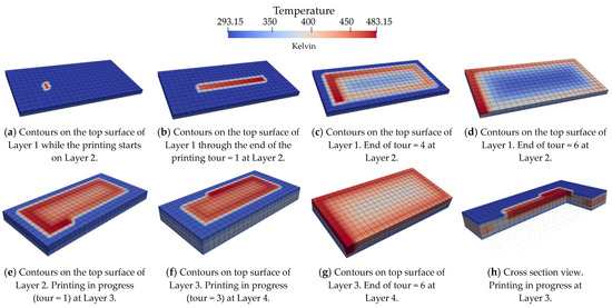
Figure 5.
Snapshots of temperatures showing change in different time intervals in 3D.
4.2. Results of Sensitivity Analyses
The results presented herein reveal how individual factors affect temperature variations, providing valuable insights into the thermal response of the 3D printing process for a defined path in Section 2.1. The location of the temperature measured is at the center of the 10th layer, where x = 0.006 m, y = 0.003 m, and z = −0.002 m.
4.2.1. Variation of Extrusion Temperature (Text)
There are two different heat transfer phenomena observed in Figure 6: temperature peaks due to the heat transfer between consecutive tours on the same layer (intralayer reheating) and temperature peaks due to heat transfer between layers (interlayer reheating).
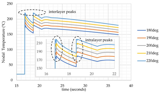
Figure 6.
Nodal temperatures under different extrusion temperatures (at the center of 10th layer).
The prompt effect of high-temperature nozzle passing from neighboring cells creates intralayer peaks in the first and second tours. However, starting from the third tour, the distance between the center node and the nozzle becomes too distant to “feel” the temperature rise caused by the extrusion. Convection from the upper surface of the center node defines the thermal response at the node. In other words, conductive heat transfer from the front, back, left, and right directions becomes insufficient to overcome convective cooling from the top surface. The reason for this mechanism is the prolonged distance from the heat source (nozzle) and the low conductivity of PLA material.
The interlayer peaks occur due to passing nozzle from neighboring cells above. Two full peaks and one slight peak (at a lower temperature than the extrusion temperature) form via conduction from the upper cells during their printing process. A slight peak shows that the rate of heat diffusion from the two layers above starts to become too distant to be sensed by the monitoring point.
Note that temperature values stay above the glass transition temperature for PLA, which is 54–56 °C [21]. Since the nodal point in Figure 6 is located at the center of the domain, it is the farthest point from the air. For different printing patterns, geometries, layer thicknesses, and printing speeds, it might be possible to observe temperatures less than Tg at the center node. For outer nodes, inside a layer, it is expected to have temperatures lower than Tg since those locations are closer to air boundaries.
4.2.2. Variation of Heat Transfer Coefficient
Heat transfer coefficients are changed between 10 W/m2-K and 100 W/m2-K for the parametric study. The 10 W/m2-K corresponds to the natural convection zone for air, and the order of 100 W/m2-K represents forced convection due to fans at the nozzle. In a study in the literature, considering the surface roughness of 3D-printed parts and different Reynolds numbers, the convective heat transfer coefficient is estimated to be within the range of 50–90 W/m2-K [23].
The rate of temperature drop between consecutive tours is affected by the change in the heat transfer coefficient (Figure 7). The third peak vanishes at high cooling rates. For the outermost nodes inside a layer, the effect of the heat transfer coefficient might be more pronounced, which may allow a faster drop below Tg.
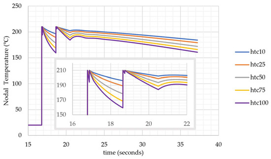
Figure 7.
Nodal temperatures under different heat transfer coefficients (at the center of 10th layer).
4.2.3. Variation of Air (Coolant) Temperature (Tair)
With the variation in the air temperature, it is observed in Figure 8 that the coolant temperature does not have a significant impact on the heat transfer at the inner nodes. A 30 °C change in the coolant temperature creates a variance of 4 °C in the nodal temperatures.
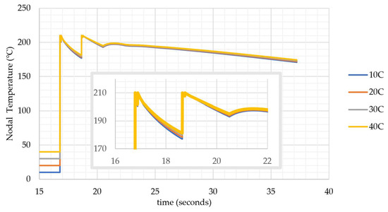
Figure 8.
Nodal temperatures under different air temperatures (at the center node of 10th layer).
For 3D printing applications, the air temperature is not expected to achieve more than 40 °C in the chamber since the total heat added to the chamber by the extrusion is roughly estimated at 24.2 °C by the well-known lumped sum heat transfer formula as follows:
Q1: Total heating provided by the hot extrusion.
Q2: Total heat received by the chamber from the extruded part.
Q1 ≈ Q2.
Q1 = 1240 kg/m3 (0.008 m × 0.006 m × 0.004 m) × 1800 J/kg-K × (210 °C − Tair).
Q2 = 1.2 kg/m3 (0.23 m × 0.19 × 0.20 m) × 1800 J/kg-K × (Tair − 20 °C).
Tair ≈ 24.2 °C
Q2 has the dimensions of the chamber, and Q1 has the dimensions of the printed part. Therefore, the maximum value that chamber air can achieve is expected to be no more than 40 °C, and within the range of the air temperature analyzed, 10–40 °C, the air temperature has no significant impact on the solution.
4.2.4. Variation of Bed Temperature (Tbed)
The impact of bed temperature on temperature history is analyzed for the bed temperature values between 40 °C and 70 °C. In Figure 9, it is seen that the bed temperature has a minor impact on the cooling pattern at the core of the geometry. Its impact slightly creates differentiation between temperature histories over time. Locations that may have temperatures close to Tg can be held above Tg for a longer period to enhance bonding.
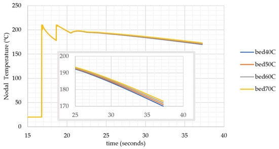
Figure 9.
Nodal temperature histories under different bed temperatures (at the center node of 10th layer).
4.3. Local Variations: Intralayer and Interlayer Analyses
The numerical results of the simulations are examined to understand how temperature varies inside individual layers (intralayer) and between layers (interlayer).
4.3.1. Intralayer Variation, Layer 4
Temperature history at nodes at different locations within the same layer is analyzed at layer 4 (Figure 10). Layer 4 is selected for this analysis since it has more layers on top to allow more time for cooling during the printing process. On the other hand, it is three cells far from the base, which serves as an adequate distance to minimize the effect of the bed temperature.
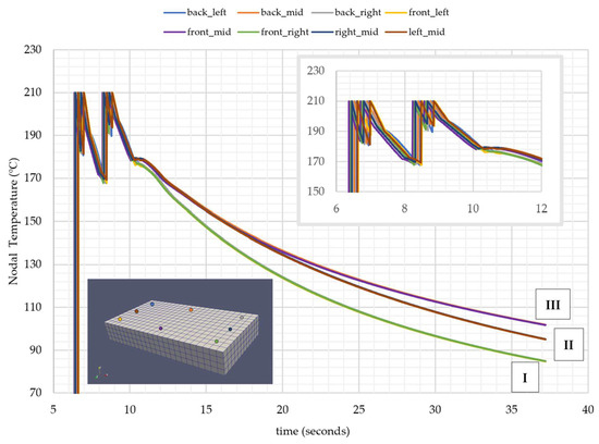
Figure 10.
Nodal temperature histories at different nodes at the same layer (4th layer).
Three distinct regimes are observed, especially during the cooling period, for nine different locations:
- (I)
- Cooling rate at corner nodes (front right, front left, back left, and back right).
- (II)
- Cooling rate at z = 2 mm (left mid, right mid).
- (III)
- Cooling rate at x = 4 mm (front mid, back mid).
This outcome shows that, despite the printing pattern having turns in the same layer, the time period between turns is not long enough to create a phase shift in the temperature history. The difference in cooling rates occurs due to dissimilar characteristic lengths on the x and y dimensions. The cooling rate is lower at locations farthest from cooling surfaces.
This phenomenon is further analyzed by comparing temperature histories on nodes aligned on a line with varying distances from the right surface. The locations of the nodes and corresponding time histories are depicted in Figure 11. Location #1 is at the innermost location of the first tour. For this reason, there is no contact with outer polymeric deposits, and hence it does not sense the extrusion temperature from other nodes, as seen in Figure 11b. Note that intralayer peak-to-peak distance increases with expanding tours since elapsed time between consecutive tours elevates because of the circling path on longer routes, i.e., elapsed time between tours 1 and 2 is longer than the one between 2 and 3 due to prolonged travel distance.
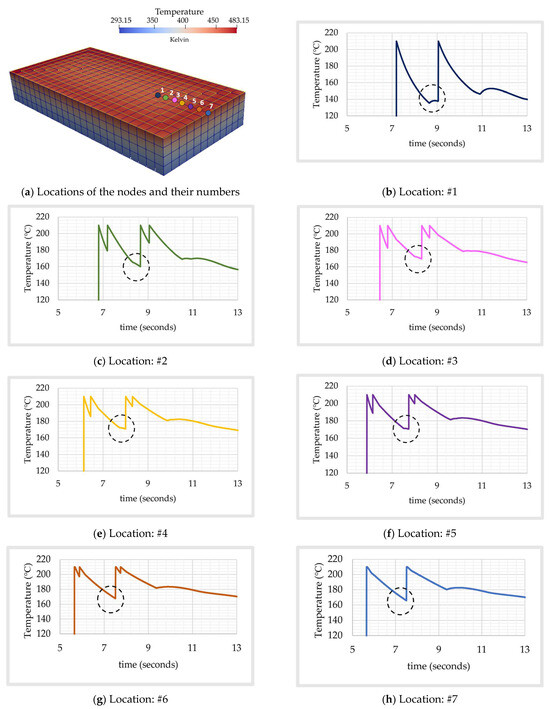
Figure 11.
Nodal temperature histories at different locations at the 4th layer. Dotted circle: instance of the third peak.
Through the end of each tour, a small and smooth peak is observed at locations #3–#7. The primary reason for these peaks is heat diffusion from the adjoint node shared with the previous tour. At Location #7, this phenomenon is even more pronounced due to the longer path and longer cooling period between tours 5 and 6. At the 1559th time step, which corresponds to t = 86.68 s, a snapshot of the geometry of an instantaneous temperature is given in Figure 12.
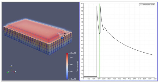
Figure 12.
Onset of diffusion from 5th tour at the 5th layer to node 7 (corner node in layer 4).
4.3.2. Interlayer Variation
In the beginning of the printing process, the bottom layers can experience lower temperatures (e.g., 70 °C for the first layer) due to the small size of the printed domain and the higher surface/volume ratio, which allows the part to cool down faster (Figure 13). And the bottom layers have more time to cool down compared to the upper layers of the printed part. The core of the part remains hot due to the concentricity of the printing pattern. For different speed, the layer thickness, geometric dimensions of the printed part, and infill ratios (e.g., 50%), the core of the part is expected to encounter lower temperatures than Tg.

Figure 13.
Nodal temperature histories at different layers (at the center of the layer). Dotted circle: lowest temperature in a layer.
Utilizing the temperature history to calculate the welding time offers insights into the degree of bonding, which can be correlated with the local distribution of Young’s modulus within the printed part. This computation is particularly relevant at locations where temperatures fall below the Tg during the printing process. However, the cases examined within the scope of this paper reveal that temperatures at most locations remain higher than Tg. Consequently, the welding time is not computed as the part layers exhibit strong bonding due to sustained temperatures above Tg. Further analyses involving varied part dimensions, printing speeds, and layer thicknesses may yield temperature histories that are more convenient for this calculation.
4.4. Effect of Printing Pattern: Concentric vs. Zigzag
The code has been modified to perform H1 (left to right) and H3 (right to left) motions to print a layer with zigzag patterns with the conditions used by Zhang et al. [14]. This pattern is numerically analyzed in the literature to estimate temperatures while printing a rectangular prism geometry with the following dimensions: 4 mm (width) × 2 mm (10 layers) × 4 mm (10 tours) on the x, y, and z axes, respectively [14].
In our investigation, we adopted identical parameters as defined in the research conducted by Zhang et al. [14]. These values are as follows: Text = 210 °C, Tbed = 60 °C, Tair = 20 °C, printing speed = 40 mm/s, and layer thickness = 0.2 mm. With these parameters, two different printing patterns, zigzag and concentric patterns, are simulated with the same discretization scheme and mesh parameters: Δx = 0.2 mm, Δy = 0.2 mm, Δz = 0.2 mm, and Δt = 5 × 10⁻³ s.
The numerical results in Figure 14 show that the pattern has a minimal impact on the maximum and minimum temperatures at a specific node. Time shifts are observed due to changes in the path. Peaks occur at different time steps since the nozzle passes at the same node at different time steps due to difference in printing paths.
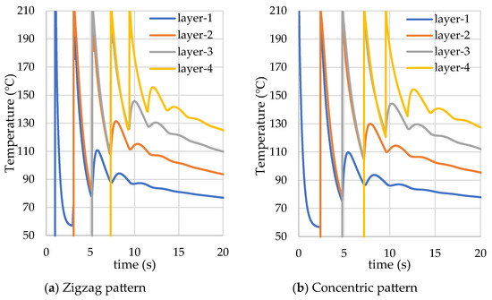
Figure 14.
Comparison between zigzag and concentric patterns at the center node.
The analyzed condition in this section yields a higher number of peaks and lower temperatures in time histories. A hand calculation is performed to reveal the main causes of this difference. The volume of the hot material added to the domain per unit time is 6 mm3/s. for a nominal case and 0.8 mm3/s. for the case analyzed for the pattern comparison. With identical cooling parameters, it is an inevitable conclusion that higher temperatures are attained when a larger volume of hot material is added to the domain per unit time.
5. Discussion
A simulation code is developed for the 3D thermal analysis of a 3D printing process. Numerical discretization methods are employed with an implicit scheme to obtain results without convergence concerns. The code is validated by using analytical results via 10-term approximation for the cooling period of a finished part as a benchmark study. The same benchmark case and corresponding conditions are modeled computationally via the developed in-house code, and a mesh study is performed to determine the mesh size that makes the solution independent from numerical errors due to discretization. With the results obtained by using the concluding mesh, it is seen that computational and analytical results are in agreement by more than 99%. Therefore, the code is used to perform thermal analyses for the 3D printing process.
A real-life printing trajectory, a concentric path from inwards to outwards with 100% infill, is defined and modeled computationally to obtain temperature history in the printed domain during the printing process. Time-dependent temperature results show peak temperature points due to the high temperature of the nozzle passing the node and the heat conducted from neighboring nodes during the process.
The analyzed printing process takes 334 time steps (equivalent to 1.86 s) to print a single layer. Due to the non-equivalent distances that the nozzle travels in different tours, the corresponding periods are as follows: the first tour is 34 time steps (0.19 s), the second is 44 time steps (0.244464 s), the third is 52 time steps (0.288912 s), the fourth is 60 time steps (0.33336 s), the fifth is 68 time steps (0.377808 s), and the sixth is 76 time steps (0.422256 s). For 20 layers, the total time is 6700 time steps (37.11408 s).
A sensitivity study is performed to investigate the effect of extrusion temperature, air temperature, bed temperature, and effective heat transfer coefficient on temperature history. In addition, results are analyzed at different locations to observe intralayer and interlayer variations. Lower temperatures are observed at the bottom layer due to more cooling time and the bed temperature boundary condition from the bottom.
The examination of temperatures at various positions on the same layer, equidistant from the nearest edge, reveals subtle variations. Notably, nodal temperatures at symmetrical locations relative to the layer’s center exhibit minor differences. This phenomenon is attributed to the compact dimensions of the geometry and the swift nozzle speed. In the case of larger parts and slower progress, where more time is allocated to traverse the same direction within a single tour, such as H1, a prolonged duration from the initiation to the conclusion of H1 may lead to the development of asymmetrical temperature patterns.
Intralayer and interlayer peaks are observed in time histories during the printing process of a layer, denoted as the nth layer. The primary interlayer peaks are a consequence of nozzle movements during the printing process at both the (n−1)th and nth layers, stemming from the extrusion boundary condition. Additionally, a third peak becomes apparent during the printing of the (n+1)th layer, attributed to conduction effects. Concerning intralayer peaks, the occurrence of two interlayer peaks is attributed to the traversal of the hot nozzle from a neighboring node during the subsequent tour. Following two consecutive tours, this peak diminishes at the monitoring point due to the amplifying cooling effects—resulting from radiative and convective heat transfer from the printed part—outweighing the conductive heating effect generated by the moving nozzle within the domain.
The extrusion temperature significantly influences the temporal evolution of temperature values, with higher nozzle temperatures resulting in elevated temperatures at the points where the nozzle traverses. Modifying the definition of tours within the in-house code offers the opportunity to analyze various printing patterns, enabling the observation of temperature histories for comparative purposes.
It is observed that nodal temperatures can fall below Tg where cooling time is longer and printed volume per unit time is smaller due to slow production speed, reduced domain size, and thinner layer thickness. Since the nodal temperatures at the inner locations of the analyzed case in this paper stay above Tg, welding time is not calculated. For the cases that allow lower temperatures than Tg, the degree of bonding (quality of bonding and strength) can be estimated with temperature history with the use of ()~()1/4 relationship given by Yang et al. [3].
Notably, the hallmark of this study lies in the conception and implementation of a proprietary, in-house code designed for the three-dimensional calculation of the heat diffusion equation tailored specifically for 3D printing applications. What sets this endeavor apart is the code’s unparalleled versatility, accommodating analysis across H1, H2, H3, and H4 directions, enabling a comprehensive examination of various printing paths. This adaptability, coupled with its seamless integration potential with a G-code, positions our approach as an invaluable tool for practical and commercial applications. As a standalone software package, this innovative solution not only advances the understanding of heat dynamics in 3D printing but also lays the foundation for real-world implementation, offering a pragmatic and sophisticated toolset for the broader scientific and industrial community.
In future work, calculating welding time under diverse printing conditions and locations offers the potential to estimate the degree of bonding. The code can be integrated with a mechanical solver to calculate warpage and optimize the parameters to prevent quality issues and scraps before the printing process (i.e., first-time right-printing opportunity). Extending the applicability of the code to analyze other additive manufacturing methods could involve modifying it to consider curing, where the heat generation term (q/k) is greater than zero. Another avenue for future research involves integrating the methodology with a g-code to analyze complex parts. To address potential challenges related to prolonged computation times in analyzing intricate components, further enhancements such as reduced order modeling, and/or the implementation of machine learning techniques can be explored as part of ongoing research efforts.
Author Contributions
Conceptualization, methodology, validation, software, visualization, writing, B.A.-T.; consultation, formal analysis, review and editing, K.K.; revisions and editing M.Ç. All authors have read and agreed to the published version of the manuscript.
Funding
This research received no external funding.
Data Availability Statement
Research data generated in scope of this article are published at https://drive.google.com/drive/folders/1NMyyezBHZsoEXxEpONYXg92ZOWpclZkC accessed on 1 February 2024.
Conflicts of Interest
The authors declare no conflicts of interest. The leading author, Buryan Turan, is also the funder of this article.
References
- Faludi, J.; Bayley, C.; Boghal, S.; Iribarne, M. Comparing environmental impacts of additive manufacturing vs. traditional machining via life-cycle assessment. Rapid Prototyp. J. 2015, 21, 14–33. [Google Scholar] [CrossRef]
- Bikas, H.; Stavropoulos, P.; Chryssolouris, G. Additive manufacturing methods and modelling approaches: A critical review. Int. J. Adv. Manuf. Technol. 2016, 83, 389–405. [Google Scholar] [CrossRef]
- Yang, F.; Pitchumani, R. Healing of thermoplastic polymers at an interface under nonisothermal conditions. Macromolecules 2002, 35, 3213–3224. [Google Scholar] [CrossRef]
- Wool, R.; O’Connor, K. A theory of crack healing in polymers. J. Appl. Phys. 1981, 52, 5953–5963. [Google Scholar] [CrossRef]
- Bartolai, J.; Simpson, J.; Xie, R. Predicting strength of additively manufactured thermoplastic polymer parts produced using material extrusion. Rapid Prototyp. J. 2018, 24, 321–332. [Google Scholar] [CrossRef]
- Edwards, S.F. The statistical mechanics of polymerized material. Proc. Phys. Soc. 1967, 92, 9–16. [Google Scholar] [CrossRef]
- Jud, K.; Kausch, H.; Williams, J. Fracture mechanics studies of crack healing and welding polymers. J. Mater. Sci. 1981, 16, 204–210. [Google Scholar] [CrossRef]
- Coogan, T.; Kazmer, D. Bond and part strength in fused deposition modeling. Rapid Prototyp. J. 2017, 23, 414–422. [Google Scholar] [CrossRef]
- Sun, Q.; Rizvi, G.; Bellehumeur, C.; Gu, P. Effect of processing conditions on the bonding quality of FDM polymer filaments. Rapid Prototyp. J. 2008, 14, 72–80. [Google Scholar] [CrossRef]
- Seppala, J.; Migler, K. Infrared thermography of welding zones produced by polymerextrusion additive manufacturing. Addit. Manuf. 2016, 12, 71–76. [Google Scholar] [PubMed]
- Coogan, T.; Kazmer, D. Healing simulation for bond strength prediction of FDM. Rapid Prototyp. J. 2017, 23, 551–561. [Google Scholar] [CrossRef]
- Yin, J.; Lu, C.; Fu, J.; Huang, Y.; Zheng, Y. Interfacial bonding during multi-material fused deposition modeling (FDM) process due to inter-molecular diffusion. Mater. Des. 2018, 150, 104–112. [Google Scholar] [CrossRef]
- Basgul, C.; Thieringer, F.M.; Kurtz, S.M. Heat transfer-based non-isothermal healing model for the interfacial bonding strength of fused filament fabricated polyetheretherketone. Addit. Manuf. 2021, 46, 102097. [Google Scholar] [CrossRef] [PubMed]
- Zhang, J.; Wang, X.Z.; Yu, W.W.; Deng, Y. Numerical investigation of the influence of process conditions on the temperature variation in fused deposition modeling. Mater. Des. 2017, 130, 59–68. [Google Scholar] [CrossRef]
- Ferraris, E.; Zhang, J.; Hooreweder, B.V. Thermography based in-process monitoring of fused filament fabrication of polymeric parts. CIRP Ann. Manuf. Technol. 2019, 68, 213–216. [Google Scholar] [CrossRef]
- Khanafer, K.; Al-Masri, A.; Deiab, I.; Vafai, K. Thermal analysis of fused deposition modeling process based finite element method: Simulation and parametric study. Numer. Heat Transf. A Appl. 2022, 81, 3–6. [Google Scholar] [CrossRef]
- Ramos, N.; Mittermeier, C.; Kiendl, J. Efficient Simulation of the Heat Transfer in Fused Filament Fabrication. J. Manuf. Process. 2023, 94, 550–563. [Google Scholar] [CrossRef]
- Mosleh, N.; Esfandeh, M.; Soheil, D. Simulation of Temperature Profile in Fused Filament Fabrication 3D Printing Method. Rapid Prototyp. J. 2024, 30, 134–144. [Google Scholar] [CrossRef]
- Chapra, S.; Canale, R. Numerical Methods for Engineers; McGraw-Hill Higher Education: Boston, MA, USA, 2010. [Google Scholar]
- Barrasa, J.O.; Ferrández-Montero, A.; Ferrari, B.; Pastor, J.Y. Characterisation and Modelling of PLA Filaments and Evolution with Time. Polymers 2021, 13, 2899. [Google Scholar] [CrossRef]
- Haleem, A.; Kumar, V.; Kumar, L. Mathematical Modelling & Pressure Drop Analysis of Fused Deposition Modelling Feed Wire. Int. J. Eng. Technol. 2017, 9, 2885–2894. [Google Scholar]
- Incropera, F.P.; Dewitt, D.P.; Bergman, T.L.; Lavine, A.S. The Plane Wall with Convection. In Fundamentals of Heat and Mass Transfer, 6th ed.; Wiley & Sons, Inc.: Hoboken, NJ, USA, 2007; pp. 272–275. [Google Scholar]
- Pereira, L.; Letcher, T.; Michna, G.J. The effects of 3d printing parameters and surface roughness on convective heat transfer performance. In Proceedings of the ASME Summer Heat Transfer Conference, Bellevue, WA, USA, 14–17 July 2019. [Google Scholar]
Disclaimer/Publisher’s Note: The statements, opinions and data contained in all publications are solely those of the individual author(s) and contributor(s) and not of MDPI and/or the editor(s). MDPI and/or the editor(s) disclaim responsibility for any injury to people or property resulting from any ideas, methods, instructions or products referred to in the content. |
© 2024 by the authors. Licensee MDPI, Basel, Switzerland. This article is an open access article distributed under the terms and conditions of the Creative Commons Attribution (CC BY) license (https://creativecommons.org/licenses/by/4.0/).