Abstract
The article presents the development of new physics-informed evolutionary neural network learning algorithms. These algorithms aim to address the challenges of ill-posed problems by constructing a population close to the Pareto front. The study focuses on comparing the algorithm’s capabilities based on three quality criteria of solutions. To evaluate the algorithms’ performance, two benchmark problems have been used. The first involved solving the Laplace equation in square regions with discontinuous boundary conditions. The second problem considered the absence of boundary conditions but with the presence of measurements. Additionally, the study investigates the influence of hyperparameters on the final results. Comparisons have been made between the proposed algorithms and standard algorithms for constructing neural networks based on physics (commonly referred to as vanilla’s algorithms). The results demonstrate the advantage of the proposed algorithms in achieving better performance when solving incorrectly posed problems. Furthermore, the proposed algorithms have the ability to identify specific solutions with the desired smoothness.
1. Introduction
The vast majority of papers presenting physics-informed neural network models and solutions use a pre-selected network architecture, mentioning that the corresponding parameters were found empirically. This dilemma is also mentioned in Haykin’s classic book [1]. The concept of architecture in this case can include both types of activation functions, the number of layers and neurons in them, and methods for initializing the output parameters of a neural network. But for its purposeful selection, it is desirable to use evolutionary algorithms [2,3,4,5,6]. These optimisation techniques utilise a set of potential solutions that evolve over time through various operations, including selection, mutation, and crossover.
The problem of determining the optimal architecture is particularly pertinent when considering neural network solutions for problems that involve differential equations [7,8]. At present, these types of neural networks are commonly referred to as Physics-Informed Neural Networks (PINNs) [9]. Although the prevailing trend in most studies involves a fixed PIN (Physics-Informed Network) architecture, a considerable number of works delve into discussions on algorithms for selecting not just weights, but also the architecture itself [10,11,12,13].
In recent years, the number of articles devoted to the search for optimal architecture has been growing. The evolutionary algorithms are employed to discover the optimal combination of weights and biases that minimise the error for a neural network are known as Grey Wolf Optimiser [14], Particle Swarm Optimiser [15] and the others [11]. The application of evolutionary algorithms to train neural networks is known as neuroevolution [16,17], which has gained attention as a promising approach for solving complex problems in various fields. The most recent studies focusing on the application of evolutionary methods for training Neural Networks are the EDEAdam algorithm [18] that combines the contemporary differential evolution technique with Adam; Enhanced colliding bodies optimization algorithms showed good results and high accuracy in [19].
One of the drawbacks of evolutionary algorithms is their significant resource intensity. Consequently, a key concern is to enhance their effectiveness. Recognising the characteristics of the problem at hand is a crucial resource for improving the efficiency of such algorithms. Additionally, a purposeful approach to population information, which encompasses a set of models involved in evolution, plays a significant role. Both of these aspects are explored in detail in this paper.
Considering the problem of population formation, it is noteworthy that constructing a Physics-Informed Neural Network (PINN) is inherently a multi-criteria task, given that boundary value problems involve multiple criteria, as they consist of an equation and boundary conditions, each of which is described by separate loss functions to assess accuracy. Additionally, when measurements are involved, an additional loss function emerges.
Typically, these individual loss functions are combined into a single function, thereby giving rise to the challenge of selecting appropriate penalty factors. Numerous approaches to addressing this problem have been proposed in the existing literature. Adaptive weights are suggested in [20], where the penalty parameter is updated at each or some steps of network training according to a predetermined formula. In [21], the weights are updated after 100 epochs of training to balance the contribution of each term. In [22], the impact of the parameter on the learning rate is assessed, and a fixed value is used to obtain the final solution. Authors of [23] examines the effect of weight on both the loss function and its individual components by comparing their values for the resulting network. In [24], the approximate solutions obtained for different values of the weight parameter are compared with the exact solution.
In this paper, we have chosen to approach the problem directly as a multi-criteria task. Solving problems with multiple objectives and multi-criteria decision making are challenges across disciplines, leading to alternative approaches beyond traditional techniques. In [25], various strategies to dynamically balance the impacts of multiple terms and gradients in the loss function by selecting the best scaling factors are explored.
Evolutionary algorithms for multi-criteria problems are considered in a number of papers. In [26], evolutionary algorithms are applied for multi-objective multi-task optimisation. The article [10] proposes an evolutionary algorithm for multi-objective architecture search that enables approximating the complete Pareto front of architectures under multiple objectives, including predictive performance and number of parameters. Evolutionary algorithms, due to their population-based nature, have been utilised to generate multiple elements of the Pareto optimal set in a single run [27]. Some practical applications to engineering problems are presented in [2]. These techniques also are well-suited for addressing challenges associated with irregular Pareto fronts [28]. It has been noticed that approaching the Pareto front [29,30] gives a set of solutions that can be regarded as a population for constructing evolutionary algorithms.
The task of building PINN was also regarded as multi-criteria. In [31], a multi-objective optimisation method for PINN training employed the non-dominated sorting algorithm is proposed and tested on simple ordinary and partial differential equation problems. In [32], it is proposed a self-adaptive gradient descent search algorithm which manually design the learning rate of different stages to match the different search stages. The evolutionary sampling algorithm dynamically evolving where collocation points over the training iterations is proposed in [33].
In this paper, the approaches mentioned above are combined. Due to the fact that evolutionary algorithms are usually resource-intensive, approaches to their acceleration are of interest. This work is devoted to the comparison of these approaches.
To evaluate the algorithms’ performance, two benchmark problems have been used. They can be attributed to the class of problems of constructing mathematical models based on heterogeneous data. Refs. [34,35,36,37] Due to the particular characteristics of the algorithms employed, it is necessary for the differential equation and the operator defining the boundary conditions to be linear. In this study, the classical Laplace equation has been chosen as the differential equation, as it is frequently utilised for testing methods designed to solve boundary value problems. Extending the algorithms to handle other linear equations generally does not introduce significant challenges.
The tasks described in this paper are classified as decision-making tasks under multi-criteria conditions. Our objective is not to construct the ultimate Pareto front, as it is typically understood in multi-objective optimization, but rather to utilize it as a mechanism that introduces the fundamental concept in the evolutionary algorithm. When modelling real objects, it is common to encounter difficulties resulting from the complex nature of the object being modelled. One such challenge is the possibility of obtaining contradictory mathematical models when describing different aspects of the object. To illustrate this, we present a benchmark example in which the solution at the corners of a square should be both 0 and 1 simultaneously. However, the continuous solution we are constructing cannot satisfy this condition, leading to significant errors in the vicinity of these points. Nevertheless, it is important to ensure that the errors are small in the rest of the area, and that our solution is consistent with the one obtained using a fundamentally different approach (in our case, the classical Fourier method). Corner singularities for initial boundary value problems have recently emerged as a topic of research interest [38,39].
Another challenge in modelling real objects is the possibility of incomplete mathematical models. In such cases, additional information can be obtained through observations of the object. In this paper, a second example is considered that highlights this challenge. Specifically, the problem consists of solving an equation without sufficient data on boundary conditions, making it impossible to obtain a correct solution using standard methods. Instead, "measurement" data is available, which does not make the problem well-posed. Computational experiment demonstrate that the proposed approach successfully regularises this problem. Both examples involve solving the Laplace equation in a closed domain. This problem is widely used as a benchmark for evaluating the performance of multi-objective evolutionary algorithms [40].
The article is structured as follows. The “Materials and Methods” section highlights the advantages of using neural network methods to model real objects, followed by a discussion of the general formulation of the modelling problem in the context of multi-criteria optimisation. The section concludes with an introduction to a family of evolutionary algorithms based on the approximation to the Pareto front. In the “Computational Methods and Results” section, we specify the problem to be solved, describe the parameters of the algorithms studied in this paper, and present their results. Section “Discussion” provides a summary of the proposed methods and a discussion of their prospects.
In [32], it is proposed a self-adaptive gradient descent search algorithm which manually design the learning rate of different stages to match the different search stages. The evolutionary sampling algorithm dynamically evolving where collocation points over the training iterations is proposed in [33].
2. Materials and Methods
2.1. Advantages of Physics-Informed Neural Network Modelling
To compare our results with previous works, it’s important to note the difference in mathematical modelling paradigms. The classical paradigm consists of three stages: first, a mathematical model of the simulated object is built based on available information, typically in the form of a differential equation (or system of equations) with additional conditions. Second, an exact or approximate solution is constructed using known numerical methods, with parameters selected to minimise error. Finally, results are interpreted and conclusions are drawn based on how well they correspond to the original object. However, this paradigm assumes perfect correspondence between the differential equation and the original object, and if results are unsatisfactory, the process must start over from the first stage.
The practicality of the following paradigm is evident. A differential equation model with additional conditions is inherently approximate. As a result, striving for very high accuracy in solving a differential problem may not be meaningful. In the second stage of this work, a set of physics-informed neural network (PINN) models is constructed to solve differential problems with varying levels of accuracy. It is crucial to obtain a sufficiently accurate solution when the differential problem corresponds to an object that requires high precision. The adaptive properties of the PINN model, such as its ability to be refined based on additional data (e.g., measurements from sensors, changes in equation parameters), are even more important. At this stage, the modest accuracy of the differential model is not a final assessment of its quality, as long as it reflects the qualitative behaviour of the solution. The differential problem should accurately reflect the qualitative behaviour of the solution, and the model should allow for refinement based on additional data.
2.2. Problem Statement
Let us examine a non-linear partial differential equation (PDE) problem, as described below
The problem under consideration may have various conditions, including boundary conditions in the form of
initial conditions in the form of
measurement data
and other conditions of different types, such as asymptotic relations [41]. Here, are some differential operators, is spatial-time coordinates, is a solution domain with a boundary , and are appropriate functions.
To solve these types of problems using neural networks, multi-objective optimisation is employed, where the losses corresponding to Equations (1)–(4) and additional conditions are minimised.
Vanilla Physics-informed neural networks [9,42] provide a solution to the problem considered in the form of a fully-connected feed-forward neural network , and the unknown parameters are found by minimising the mean squared error losses over the space of these parameters,
These multiple loss functions, residual loss, initial loss, boundary loss, and data loss for inverse problems, are employed in PINNs. To train PINNs, the most common method is to optimise the total loss, which is a weighted sum of the loss functions, using standard stochastic gradient descent algorithms. The classical approach offers several options for constructing general loss functions using the method of linearisation for multi-objective optimisation problems. These options include varying the number of collocation points used to calculate the discrepancy for Equations (1)–(3), the volumes of training and test set () for measurement data, and the inclusion,
or exclusion [9],
of penalty multipliers for the terms in the general loss function. Selecting an appropriate penalty parameter is a crucial task, and various approaches have been proposed in the literature.
Next, we propose the general idea of an evolutionary algorithm for solving multi-criteria decision making problems. The Pareto front principle is one of the important components of this algorithm.
2.3. Evolutionary Algorithms Based on Pareto Front: General Idea
In this scientific paper, we investigate the use of evolutionary algorithms to train physics-informed neural networks based on the Pareto front. Our proposed approach involves incorporating schemes of mutation, crossover, and selection of individuals based on specific criteria. As criteria, the loss functions (1)–(4) presented earlier can be used, as well as expert knowledge or any information that becomes available in real-time.
To account for the multi-objective nature of the optimisation problem, we vary the penalty factor in the loss function. By training separate solutions for different penalty factor values, we generate an analogue of the Pareto front and select the best instances using a chosen criterion. To implement the principle of survival of the fittest individuals from the population, our evolutionary algorithm selectively chooses individuals from the initial population for mutation.
To illustrate the underlying concept, we assume that represent different criteria for decision making, such as loss functions, logical indicators, or custom-designed functions [43].
Figure 1 shows the mutation procedure used in our family of evolutionary algorithms, called the Pareto Mutation.
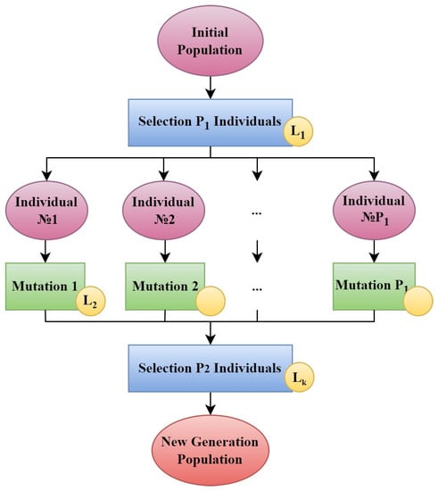
Figure 1.
Evolutionary interpretation of Pareto mutation. The diagram showcases the construction of an analogue of the Pareto front of solutions, as well as the selection of a new generation of solutions through evolutionary processes. The yellow circles represent locations where specific problem criteria are incorporated by individuals’ evaluation.The training of PINNs is considered as Mutation 1–Mutation .
Then the Pareto mutation is incorporated into the overall framework. It’s worth noting that specific criteria are employed both at various stages of the general algorithm, as shown in Figure 2, and within the Pareto Mutation. The points of variation are indicated by yellow circles. The dotted line represents the expansion of the scheme, which is beyond the scope of this paper. The overall structure of the scheme follows a standard pattern observed in evolutionary algorithms. For instance, one can refer to the scheme of the optimization genetic algorithm process for artificial neural networks presented in [44] as an example.
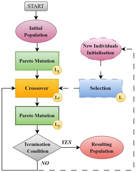
Figure 2.
The evolutionary algorithm used for generating a PINN solution population. The yellow circles represent locations where specific problem criteria are incorporated by individuals’ evaluation. The ‘Crossover’ refers to the process of introducing additional neurons to the current generation of PINNs.
Assuming a general scheme for a family of evolutionary algorithms based on the criteria outlined in conditions (1)–(4), various algorithms can be developed using criteria such as (5)–(8) or others. The properties of solutions generated by these algorithms and the impact of neural network hyper-parameters on these solutions are promising research areas. This article addresses ill-posed tasks that present challenges when solved using vanilla PINNs.
3. Computational Experiments and Results
3.1. Benchmark Problems Statement
Let us examine one benchmark problem—specifically, the Laplace equation
with discontinuous Dirichlet boundary conditions
and the same Laplace equation that lacks boundary or initial conditions but includes additional data that simulates measurements
The considered problems have already been solved by other methods [12,13,43], they seem to us convenient for comparative testing of algorithms.
When approaching tasks (10)+(11) and (10)+(12) using a general neural network approach [9,42], the optimal choice is an RBF network with radial activation functions. This is due to the closed domain on which the Laplace operator is calculated, where values outside this set are not needed, as opposed to a multilayer perceptron which implies the need for determining values beyond the boundaries. Radial basis functions are well-suited for local approximation in a small neighbourhood of each point, making them an ideal choice for these tasks.
It should be noted that, in all experiments, fixed collocation points have been used at the boundaries, and randomly distributed and resampled points have been employed within the region after a fixed number of training epochs to train the network.
3.2. Algorithms Description
A disadvantage of the classical solution of the problem (10)+(11) using the Fourier method is the Gibbs effect on the boundary. The largest discrepancy between the Fourier solution and the problem condition occurs when computing the root-mean-square error of the function’s derivative error of satisfying the derivative equal to zero at the trial points on the upper boundary of the square. When computed at 1000 randomly chosen points, it has an approximate magnitude of 40. Therefore, the constancy condition of the function and the equality of the function’s derivative to zero at the boundary are regarded as additional criteria for evaluating the solution.
In this paper, algorithms are examined that result in the smoothest solutions being constructed at the domain boundary based on these considerations.
This subsection describes the specific parameters of the algorithms and hyper-parameters of neural networks used in the computational experiments. The scheme for the entire family of algorithms presented in Figure 2 is followed, as well as the scheme for the Pareto mutation depicted in Figure 1.
- Termination condition:The method terminates after achieving a predefined number of neurons, N, in a PINN model. Different values of N are considered to investigate the impact of the total number of neurons on the obtained solutions and their outcomes.
- Initial PopulationA population of neurons with radial basis functions of the formis randomly initialised as the initial population. Here, . Subsequently, all individuals are fed into the input of the Pareto mutation process. The value is quite small, but provides a stable penalty multiplier value (14) for Pareto mutation.
- Pareto Mutation:To select individuals from the incoming population, the following procedure is employed. During the initial mutation, the discrete quadratic errors for satisfying the Laplace equation and boundary conditions are calculated for each initialised network. These errors are then summed to derive a "global" penalty multiplierfor the linearised loss function , and where is the number of different mutations (see Figure 1). Afterwards, for each subsequent mutation , an individual is selected based on having the lowest loss .During the mutation process, the current networks are trained independently by minimising the corresponding loss functions using algorithm Rprop [45] and by regenerating points for the Laplace equation every 5 training epochs. The total number of training epochs can be selected separately. For the last mutation, The total number of training epochs is employed. The values considered in the experiments are presented in Table 1.
 Regarding the second selection procedure outlined in the Pareto mutation, all mutated networks are preserved in all runs () except for the final one.As previously mentioned, collocation points are utilised at the boundary. Initially, they are split into two sets: the first set is involved in the training of the network, while the second set is employed in the selection process. Except for the first mutation, all other mutations employ the first set of points for training PINNs.
 - Crossover:The present study investigates algorithm that employs crossover within the current population. The optimal Pareto set for this PINN solutions is constructed based on the discrete quadratic errors for satisfying the Laplace equation and boundary conditions . Next, the neurons are selected from individuals located at the leftmost and rightmost ends of the current Pareto-optimal set, and added one by one to all other networks multiplied by the optimal parameter in the sense of least squares. From the resulting new individuals, the one with the minimum error is selected for each value of the penalty multiplier , A scheme of the Crossover procedure is presented in Figure 3.
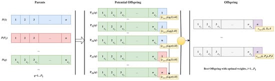 Figure 3. A scheme of ’Crossover’ procedure. and are the leftmost and rightmost ends of the current Pareto-optimal set with n neurons; are current population of PINNs with extrernal multiplier (weight) of each neuron. are optimal external weights of new neuron minimising corresponding error . The yellow circle represents incorporating specific problem criteria by individuals’ evaluation.
 - A note on the set of penalty multipliers:In the previous paragraph, we introduced two different sets of penalty multipliers. The general scheme of the algorithm allows for new selections of such sets within each mutation and crossover. In this study, we consider two options: in the first, the set of penalty multipliers is fixed during the initialisation of the first population of networks (), while in the second, parameter is updated during the crossover process. In the latter case, the new parameter is calculated as follows:where and are the numbers of individuals from the leftmost and rightmost ends of the current Pareto-optimal set.
Table 1 displays the parameter values of the described algorithm across different variants. The parameter values were chosen to strike a balance between stability and the duration of computational experiments. For instance, using individuals in the current population undergoing independent Pareto mutations yielded the same result as using , while significantly reducing the execution time. Further reduction of threads resulted in inferior outcomes.
3.3. Results: Problem (10)+(11)
The restart method was applied to the three algorithm variations described in Figure 2 and above, with the parameters presented in Table 1, in a series of experiments. Different variants of Algorithm 1 have been utilised. Algorithm 1_1 involves updating the set of penalty factors, while Algorithm 1_3 stores the values obtained during the initialisation stage of the initial population. One of the variants of Algorithm 1, Algorithm 1_2 incorporates an evolutionary mechanism for updating the PINN model’s weights. During the Pareto mutation, some weights are replaced by the nearest elements of the current Pareto-optimal set.
| Algorithm 1 Evolutionary PINN Learning Algorithms Inspired by Approximation to Pareto Front |
|
Solutions minimising expressions (5), (6) and
have been selected from the final Pareto-optimal set if PINN solutions to evaluate the results. The effectiveness of the latter criterion has been demonstrated in prior studies of similar problems. In addition, upper bounds have been introduced for characteristics (5) and (6). The nonparametric Kruskal-Wallis and Mann-Whitney tests were primarily used to analyse the results. Unless otherwise specified, significant differences were determined at the 0.05 level.
We investigate the effect of the number of neurons N in the final solution on the quality of solutions obtained using all types of algorithm. Figure 4 indicates that solutions with and 30 approximate the Pareto front. Additionally, for Algorithm 1_3, there is a significant difference in characteristics (5) and (6) at a significance level of 0.05.
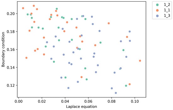
When comparing the results of the algorithms themselves, Figure 5 shows that maintaining a diverse range of solutions within the obtained set is especially observed in the case of Algorithms 1_1 and 1_2 significant difference in the values of characteristics (5) and (6) at the 0.05 significance level. It should be noted that when considering all solutions obtained, Algorithms 1_1 and 1_2 tend to increase the importance of meeting the Laplace equation criterion.
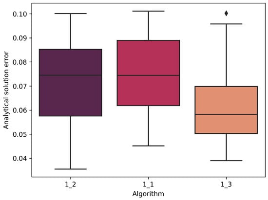
The experimental results indicate that the Pareto-optimal solutions correspond to the smallest discrepancies with the analytical solution obtained by the Fourier method, which confirms the consistency of methods being evaluated. There is a statistically significant difference between the outcome of Algorithm 1_3 and that of Algorithms 1_1 and 1_2, that is evident in Figure 6. Algorithm 1_3 is the only one for which the compliance with the analytical solution is affected by the number of neurons in the resulting network. Specifically, models with 10 neurons yield significantly worse results compared to those with 20 and 30 neurons.
Regarding the influence of hyperparameters, such as the number of epochs for PINN training at different algorithm steps, no effect on compliance with the analytical solution was observed.
As previously mentioned, in addition to the primary criteria for selecting the best solution, the error of satisfying the derivative equal to zero on the boundary can also be taken into consideration.
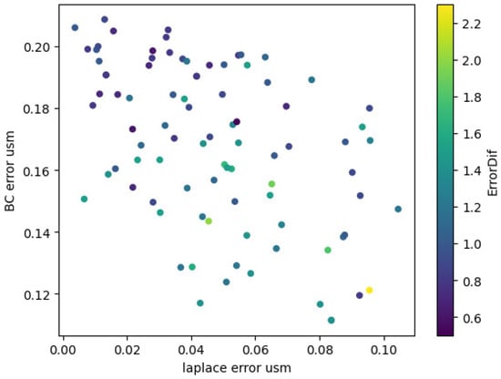
Upon analysing the general scattering diagram depicted in Figure 7, we observe that the smoothest on the upper boundary solutions do not belong to the Pareto-optimal set. Additionally, the maximum value of this criterion is 2, which is significantly lower than the value of 40 obtained for the analytical solution using the Fourier method. Furthermore, Algorithm 1_3 yield significantly worse results compared to Algorithms 1_1 and 1_2. Additionally, this trend becomes more pronounced as the number of neurons increases. We did not observe any impact on the adherence to the analytical solution when varying the number of epochs for PINN training.
3.4. Results: Problem (10)+(12)
As a reminder, the second set of experiments involves solving a problem without boundary conditions, where measurement data is incorporated as a secondary criterion to the Laplace equation. Computational experiments were carried out for the algorithm parameters presented in Table 2. Algorithm 1_1 is used for this task due to its lower susceptibility to retraining at collocation points.
The exact measurement data is obtained by solving the Laplace equation analytically using the Fourier method. To simulate measurement with error, a uniformly distributed random variable t on the interval [−1, 1] is added to the analytical solution using formula
To prevent overfitting, the measurement points are distributed on a pseudo-uniform grid inside the square, with a random shift applied to the grid.
Half of the measurement points are allocated for training, while the remaining half is used to select the best individuals during the crossover process and the optimal solution in the final cycle of the algorithm.
Five runs of the computational experiment have been performed for each algorithm parameter configuration and measurement data parameter set. The optimal Pareto set among all solutions consists of neural networks that stopped training at neurons.
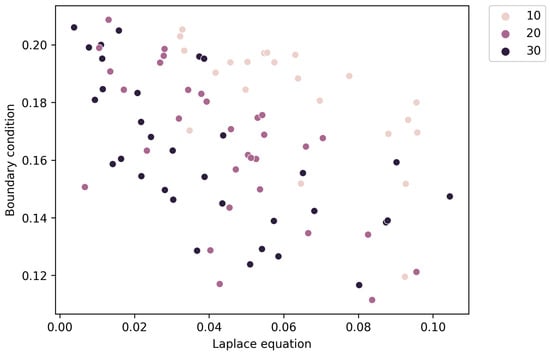
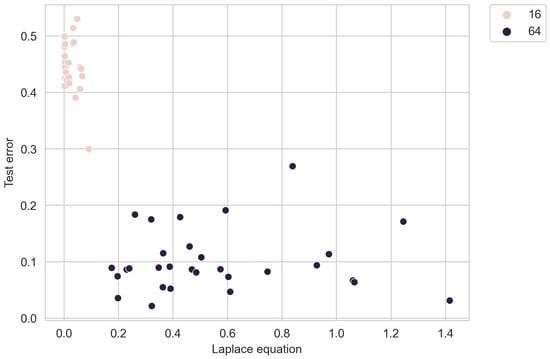
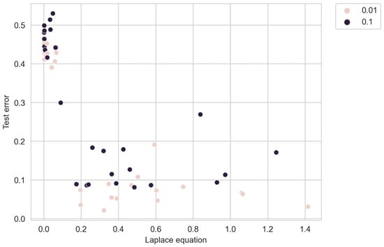
Figure 8 illustrates how the algorithm places greater importance on satisfying the desired solution of the Laplace equation with fewer measurements.
In general, there were no significant differences observed across different noise levels, indicating that the algorithm is robust to errors in measurements. This is illustrated in Figure 9. Furthermore, a large error in the data has no impact on the error in satisfying the exact solution.
To compare with standard networks, we trained a network of 30 neurons on a linearised loss function with a fixed penalty multiplier calculated during initialisation. However, none of the obtained solutions fell within the target range due to retraining towards one of the terms, which was influenced by the initial random values of the network weights.
4. Discussion
In this article, we have explored the use of evolutionary algorithm to construct physics-informed neural network models for real objects, which presents some challenges in their description. One example highlights the difficulties arising from a contradictory mathematical model containing differential equations and boundary conditions. Another example, which we analyse in this paper, involves the absence of a complete mathematical model for the object, which is addressed by incorporating observational data. The tasks discussed in this paper are categorized as decision-making tasks in multi-criteria scenarios. Our goal is not to construct the ultimate Pareto front, as it is typically defined in multi-objective optimization, but rather to employ it as a mechanism that introduces the fundamental concept in the evolutionary algorithm.
The study has demonstrated that the proposed algorithm can incorporate various criteria during both the training and selection stages of model populations. Increasing the total number of neurons in the model enhances the quality of solutions, while parallel training of individuals enables the emphasis on specific criteria or the attainment of solutions with desired smoothness. All models from the Pareto optimal set exhibit the best agreement with the analytical solution obtained by the Fourier method, and the stability of the solutions to increasing measurement errors is also observed.
Future research can investigate the properties of this evolutionary algorithm family on other types of ill-posed problems.
Author Contributions
Conceptualization, T.L. and D.T.; methodology, T.L. and D.T.; software, D.T.; validation, T.L., D.T., M.C., E.R., A.S. and T.S.; formal analysis, T.L.; investigation, T.L., D.T., M.C., E.R., A.S. and T.S.; resources, T.L., D.T., M.C., E.R., A.S. and T.S.; data curation, T.L. and D.T.; writing—original draft preparation, T.L.; writing—review and editing, T.L. and D.T.; visualization, T.L.; supervision, T.L. and D.T.; project administration, T.L. and D.T.; funding acquisition, D.T. All authors have read and agreed to the published version of the manuscript.
Funding
This work was supported by the Russian Science Foundation under grant No. 22-21-20004, https://rscf.ru/project/22-21-20004/ (accessed on 18 August 2023).
Institutional Review Board Statement
Not applicable.
Informed Consent Statement
Not applicable.
Data Availability Statement
Data available on request from the authors.
Conflicts of Interest
The authors declare no conflict of interest.
Abbreviations
The following abbreviations are used in this manuscript:
| PINN | physics-informed neural network |
References
- Haykin, S. Neural Networks: A Comprehensive Foundation; Prentice Hall: Hoboken, NJ, USA, 1999; 842p. [Google Scholar]
- Slowik, A.; Kwasnicka, H. Evolutionary algorithms and their applications to engineering problems. Neural Comput. Appl. 2020, 32, 12363–12379. [Google Scholar] [CrossRef]
- Maier, H.R.; Razavi, S.; Kapelan, Z.; Matott, L.S.; Kasprzyk, J.; Tolson, B.A. Introductory overview: Optimization using evolutionary algorithms and other metaheuristics. Environ. Model. Softw. 2019, 114, 195–213. [Google Scholar] [CrossRef]
- Yu, X.; Gen, M. Introduction to Evolutionary Algorithms; Springer Science & Business Media: London, UK, 2010. [Google Scholar]
- Tian, Y.; Zhang, X.; Wang, C.; Jin, Y. An Evolutionary Algorithm for Large-Scale Sparse Multiobjective Optimization Problems. IEEE Trans. Evolut. Comput. 2020, 24, 2380–2393. [Google Scholar] [CrossRef]
- Sirignano, J.; Spiliopoulos, K. DGM: A deep learning algorithm for solving partial differential equations. J. Comput. Phys. 2018, 375, 1339–1364. [Google Scholar] [CrossRef]
- Dissanayake, M.W.M.G.; Phan-Thien, N. Neural-network-based approximations for solving partial differential equations. Commun. Numer. Methods Eng. 1994, 10, 195–201. [Google Scholar] [CrossRef]
- Lagaris, I.; Likas, A.; Fotiadis, D. Artificial neural networks for solving ordinary and partial differential equations. IEEE Trans. Neural Netw. 1998, 9, 987–1000. [Google Scholar] [CrossRef]
- Raissi, M.; Perdikaris, P.; Karniadakis, G.E. Physics-informed neural networks: A deep learning framework for solving forward and inverse problems involving nonlinear partial differential equations. J. Comput. Phys. 2019, 378, 686–707. [Google Scholar] [CrossRef]
- Elsken, T.; Metzen, J.H.; Hutter, F. Efficient Multi-Objective Neural Architecture Search via Lamarckian Evolution. arXiv 2018, arXiv:1804.09081. [Google Scholar]
- Vasilyev, A.N.; Tarkhov, D.A. Mathematical models of complex systems on the basis of artificial neural networks. Nonlinear Phenom. Complex Syst. 2014, 17, 327–335. [Google Scholar]
- Tarkhov, D.A. Neural networks as a means of mathematical modeling. Neurocomput. Dev. Appl. 2006, 2, 1–49. [Google Scholar]
- Tarkhov, D.; Vasilyev, A.N. Semi-Empirical Neural Network Modeling and Digital Twins Development; Academic Press: Cambridge, MA, USA, 2019. [Google Scholar]
- Mirjalili, S.; Mirjalili, S.M.; Lewis, A. Grey Wolf optimizer. Adv. Eng. Softw. 2014, 69, 46–61. [Google Scholar] [CrossRef]
- Eberhart, R.; Kennedy, J. Particle swarm optimization. In Proceedings of the ICNN’95—International Conference on Neural Networks, Perth, WA, Australia, 27 November–1 December 1995; Volume 4, pp. 1942–1948. [Google Scholar]
- Stanley, K.; Clune, J.; Lehman, J.; Miikkulainen, R. Designing neural networks through neuroevolution. Nat. Mach. Intell. 2019, 1, 24–35. [Google Scholar] [CrossRef]
- Soltoggio, A.; Stanley, K.O.; Risi, S. Born to learn: The inspiration, progress, and future of evolved plastic artificial neural networks. Neural Netw. 2018, 108, 48–67. [Google Scholar] [CrossRef] [PubMed]
- Xue, Y.; Tong, Y.; Neri, F. An ensemble of differential evolution and Adam for training feed-forward neural networks. Inf. Sci. 2022, 608, 453–471. [Google Scholar] [CrossRef]
- Kaveh, A.; Khavaninzadeh, N. Efficient training of two ANNs using four meta-heuristic algorithms for predicting the FRP strength. Structures 2023, 52, 256–272. [Google Scholar] [CrossRef]
- Basir, S.; Inanc, S. Physics and Equality Constrained Artificial Neural Networks: Application to Partial Differential Equations. arXiv 2021, arXiv:2109.14860. [Google Scholar]
- Zobeiry, N.; Humfeld, K.D. A Physics-Informed Machine Learning Approach for Solving Heat Transfer Equation in Advanced Manufacturing and Engineering Applications. Eng. Appl. Artif. Intell. 2021, 101, 104232. [Google Scholar] [CrossRef]
- Rao, C.; Sun, H.; Liu, Y. Physics-informed deep learning for incompressible laminar flows. arXiv 2020, arXiv:2002.10558. [Google Scholar] [CrossRef]
- Huang, Y.; Zhang, Z.; Zhang, X. A Direct-Forcing Immersed Boundary Method for Incompressible Flows Based on Physics-Informed Neural Network. Fluids 2022, 7, 56. [Google Scholar] [CrossRef]
- Wang, H.; Liu, Y.; Wang, S. Dense velocity reconstruction from particle image velocimetry/particle tracking velocimetry using a physics-informed neural network. Phys. Fluids 2022, 34, 017116. [Google Scholar] [CrossRef]
- Bischof, R.; Kraus, M. Multi-objective loss balancing for physics-informed deep learning. arXiv 2021, arXiv:2110.09813. [Google Scholar]
- Du, K.J.; Li, J.Y.; Wang, H.; Zhang, J. Multi-objective multi-criteria evolutionary algorithm for multi-objective multi-task optimization. Complex Intell. Syst. 2022, 9, 1211–1228. [Google Scholar] [CrossRef]
- Coello, C.A.C.; Lamont, G.B.; Van Veldhuizen, D.A. Evolutionary Algorithms for Solving Multi-Objective Problems, 2nd ed.; Springer: New York, NY, USA, 2007. [Google Scholar]
- Liu, Q.; Jin, Y.; Heiderich, M.; Rodemann, T.; Yu, G. An Adaptive Reference Vector-Guided Evolutionary Algorithm Using Growing Neural Gas for Many-Objective Optimization of Irregular Problems. IEEE Trans. Cybern. 2020, 52, 2698–2711. [Google Scholar] [CrossRef]
- Lin, X.; Zhen, H.; Li, Z.; Zhang, Q.; Kwong, S.T. Pareto Multi-Task Learning. arXiv 2019, arXiv:1912.12854. [Google Scholar]
- Momma, M.; Dong, C.; Liu, J. A Multi-objective / Multi-task Learning Framework Induced by Pareto Stationarity. In Proceedings of the 39th International Conference on Machine Learning (PMLR), Baltimore, MD, USA, 17–23 July 2022; Volume 162, pp. 15895–15907. [Google Scholar]
- Lu, B.; Moya, C.; Lin, G. NSGA-PINN: A Multi-Objective Optimization Method for Physics-Informed Neural Network Training. Algorithms 2023, 16, 194. [Google Scholar] [CrossRef]
- Xue, Y.; Wang, Y.; Liang, J. A self-adaptive gradient descent search algorithm for fully-connected neural networks. Neurocomputing 2022, 478, 70–80. [Google Scholar] [CrossRef]
- Daw, A.; Bu, J.; Wang, S.; Perdikaris, P.; Karpatne, A. Rethinking the importance of sampling in physics-informed neural networks. arXiv 2022, arXiv:2207.02338. [Google Scholar]
- Cauteruccio, F.; Stamile, C.; Terracina, G.; Ursino, G.; Sappey-Mariniery, D. An automated string-based approach to White Matter fiber-bundles clustering. In Proceedings of the 2015 International Joint Conference on Neural Networks (IJCNN), Killarney, Ireland, 12–17 July 2015. [Google Scholar] [CrossRef]
- He, Q.; Barajas-Solano, D.; Tartakovsky, G.; Tartakovsky, A.M. Physics-informed neural networks for multiphysics data assimilation with application to subsurface transport. Adv. Water Resour. 2020, 141, 103610. [Google Scholar] [CrossRef]
- Viguerie, A.; Lorenzo, G.; Auricchio, F.; Baroli, D.; Hughes, T.J.R.; Patton, A.; Reali, A.; Yankeelov, T.E.; Veneziani, A. Simulating the spread of COVID-19 via a spatially-resolved susceptible–exposed–infected–recovered–deceased (SEIRD) model with heterogeneous diffusion. Appl. Math. Lett. 2021, 111, 106617. [Google Scholar] [CrossRef] [PubMed]
- Calimeri, F.; Cauteruccio, F.; Cinelli, L.; Marzullo, A.; Stamile, C.; Terracina, G.; Durand-Dubief, F.; Sappey-Marinier, D. A logic-based framework leveraging neural networks for studying the evolution of neurological disorders. Theory Pract. Logic Programm. 2021, 21, 80–124. [Google Scholar] [CrossRef]
- Trogdon, T.; Biondini, G. Evolution partial differential equations with discontinuous data. Quart. Appl. Math. 2019, 77, 689–726. [Google Scholar] [CrossRef]
- Mitchell, S.L.; Vynnycky, M. An accuracy-preserving numerical scheme for parabolic partial differential equations subject to discontinuities in boundary conditions. Appl. Math. Comput. 2021, 400, 125979. [Google Scholar] [CrossRef]
- Araújo, A.; Martins, F.; Vélez, W.; Portela, A. Automatic mesh-free boundary analysis: Multi-objective optimization. Eng. Anal. Bound. Elem. 2021, 125, 264–279. [Google Scholar] [CrossRef]
- Lazovskaya, T.; Tarkhov, D. Fresh approaches to the construction of parameterized neural network solutions of a stiff differential equation. St. Petersburg Polytech. Univ. J. Phys. Math. 2015, 1, 192–198. [Google Scholar] [CrossRef][Green Version]
- Tarkhov, D.; Vasilyev, A. New neural network technique to the numerical solution of mathematical physics problems. II: Complicated and nonstandard problems. Opt. Mem. Neural Netw. (Inf. Opt.) 2005, 14, 97–122. [Google Scholar]
- Lazovskaya, T.; Tarkhov, D.; Dudnik, A.; Koksharova, E.; Mochalova, O.; Muranov, D.; Pozhvanyuk, K.; Sysoeva, A. Investigation of Pareto Front of Neural Network Approximation of Solution of Laplace Equation in Two Statements: With Discontinuous Initial Conditions or with Measurement Data. In Advances in Neural Computation, Machine Learning, and Cognitive Research VI. NEUROINFORMATICS 2022; Kryzhanovsky, B., Dunin-Barkowski, W., Redko, V., Tiumentsev, Y., Eds.; Studies in Computational Intelligence; Springer: Cham, Switzerland, 2023; Volume 1064. [Google Scholar] [CrossRef]
- Satrio, P.; Mahlia, T.M.I.; Giannetti, N.; Saito, K. Optimization of HVAC system energy consumption in a building using artificial neural network and multi-objective genetic algorithm. Sustain. Energy Technol. Assess. 2019, 35, 48–57. [Google Scholar] [CrossRef]
- Braun, H.; Riedmiller, M. A direct adaptive method for faster backpropagation learning: The Rprop algorithm. In Proceedings of the IEEE International Conference on Neural Networks, San Francisco, CA, USA, 28 March–1 April 1993; pp. 586–591. [Google Scholar]
Disclaimer/Publisher’s Note: The statements, opinions and data contained in all publications are solely those of the individual author(s) and contributor(s) and not of MDPI and/or the editor(s). MDPI and/or the editor(s) disclaim responsibility for any injury to people or property resulting from any ideas, methods, instructions or products referred to in the content. |
© 2023 by the authors. Licensee MDPI, Basel, Switzerland. This article is an open access article distributed under the terms and conditions of the Creative Commons Attribution (CC BY) license (https://creativecommons.org/licenses/by/4.0/).