The Complexity of the Super Subdivision of Cycle-Related Graphs Using Block Matrices

Abstract

The complexity (number of spanning trees) in a finite graph $\Gamma$ (network) is crucial. The quantity of spanning trees is a fundamental indicator for assessing the dependability of a network. The best and most dependable network is the one with the most spanning trees. In graph theory, one constantly strives to create novel structures from existing ones. The super subdivision operation produces more complicated networks, and the matrices of these networks can be divided into block matrices. Using methods from linear algebra and the characteristics of block matrices, we derive explicit formulas for determining the complexity of the super subdivision of a certain family of graphs, including the cycle $C_n$, where $n=3,4,5,6$; the dumbbell graph $D{b}_{m,n}$; the dragon graph $P_m\left(C_n\right)$; the prism graph ${\Pi }_n$, where $n=3,4$; the cycle $C_n$ with a $P_{\frac{n}{2}}$-chord, where $n=4,6$; and the complete graph $K_4$. Additionally, 3D plots that were created using our results serve as illustrations.

1. Introduction

Graph theory is a theory that merges mathematics with computer technology. For a simple, undirected and connected graph $\Gamma =\left(V\right(\Gamma ),E(\Gamma \left)\right)$, a spanning tree is a subset of the edges of $\Gamma$ that connect all the vertices together without any cycles [1]. The complexity of $\Gamma$, denoted by $\tau (\Gamma )$, is the total number of spanning trees existent therein. It is used to calculate the connected and acyclic components that are present in it. Spanning trees are well recognised, and several studies have been conducted to prove their existence and count all of their numbers. One can introduce the complexity function $\tau (\Gamma )=\tau \left(\kappa \right)$ for an infinite family of graphs ${\Gamma }_{\kappa },\kappa \in \mathbb{N},$ which makes it much easier to calculate and identify the number of corresponding spanning trees, especially when these numbers are very large. The number of spanning trees is employed in a variety of fields, including engineering and network reliability. This invariantly contributes to enhancing the robustness of wireless sensor networks (WSNs) and other analogous mobile networks. The security plan for a building’s sensitive area is an example of another way complexity is used.

One of the biggest chemistry challenges is correctly recognising a chemical molecule. In [2], Joita et al. introduced graph representations of molecules as well as answers to questions about relationships between the structure of chemical compounds and various parameters. The number of spanning trees is employed in the field of chemistry. In [3,4], Nikolić et al. studied the complexity of molecules using approaches based on the topological complexity, that is, the complexity of the corresponding molecular graphs. Several measures of the topological complexity, such as those introduced by Bertz and Randić or based on the number of spanning trees, have been studied and a comparison was made between these measures of topological complexity for selected molecular graphs. For more details, please refer to [5,6,7].

A different way of displaying and condensing data from graphs is via matrices. The same information is contained in both a matrix and a graph, but a matrix is more effective for computing and computer analysis [8]. Given a graph $\Gamma =\left(V\right(\Gamma ),E(\Gamma \left)\right)$ with $\left|V\right(\Gamma \left)\right|=\kappa$, the adjacency matrix of $\Gamma$ denoted by $A(\Gamma )=a_{\ell m}$ is a $\kappa \times \kappa$ matrix defined as follows. The rows and the columns of $A(\Gamma )$ are indexed by $V(\Gamma )$. If $\ell \ne m$, then the $(\ell ,m)$ -entry of $A(\Gamma )$ is 0 for nonadjacent vertices ℓ and m, and the $(\ell ,m)$-entry is 1 for adjacent ℓ and $m$. The $(\ell ,\ell )$-entry of $A(\Gamma )$ is 0 for $\ell =1,\cdots ,\kappa$, i.e.,

$$a_{\ell m}:=\left\{\begin{array}{cc}1\hfill & \mathrm{if}{v}_{\ell }{v}_m\in E(\Gamma ),\hfill \\ 0\hfill & \mathrm{if}\mathrm{otherwise}.\hfill \end{array}\right.$$

The degree matrix [8] D for $\Gamma$ is a $\kappa \times \kappa$ diagonal matrix defined as

$$D_{\ell m}:=\left\{\begin{array}{cc}deg\left(v_{\ell }\right)\hfill & \mathrm{if}\ell =m,\hfill \\ 0\hfill & \mathrm{if}\mathrm{otherwise}.\hfill \end{array}\right.$$

where the vertex’s degree $deg\left(v_{\ell }\right)$ is the number of times an edge ends at that vertex.

The Laplace matrix of $\Gamma$ denoted by $L(\Gamma )$ is defined as $D(\Gamma )-A(\Gamma )$. It is well known that $L(\Gamma )$ is a positive semidefinite matrix with the smallest eigenvalue 0. Kirchhoff presented the first method to calculate the number of spanning trees defined as the matrix tree theorem [9], which says that all the cofactors of L are equal and their common value is equal to the complexity $\tau (\Gamma )$ of $\Gamma$.

Temperley [10] has shown that

$$\tau (\Gamma )=\frac{1}{{\kappa }^2}det(L+J),$$

(1)

where J is a $\kappa \times \kappa$ matrix, all of whose elements are ones.

Brownaj et al. [11] applied various methods to calculate the complexities of graphs that represent fullerenes ($C_{60}$, $C_{70}$ and $C_{120}$ molecules). These graphs are large, regular and highly symmetrical. Kirby et al. [12] presented a theorem called the cycle theorem, by means of which the complexity of a labelled planar or non-planar graph may be calculated from, in general, two determinants. These are much smaller than in the traditional matrix tree theorem. They applied this theorem to a conventional toroidal polyhex.

The contraction–deletion theorem is one of the most often used techniques for determining complexity. The complexity $\tau (\Gamma )$ of a graph $\Gamma$ is equal to $\tau (\Gamma )=\tau (\Gamma -x)+\tau (\Gamma /x)$, where x is any edge of $\Gamma$, $\Gamma -x$ is the deletion of x from $\Gamma$ and $\Gamma /x$ is the contraction of x in $\Gamma$. This provides a recursive way to determine how complex a graph is, see [13].

Another significant technique is using electrically equivalent transformations of networks. Zhang et al. [14] discovered a clear-form formula for the enumeration of spanning trees of the subdivided line graph of a simple connected graph using the theory of electrical networks. Teufl and Wagner [15] have demonstrated that the number of spanning trees in a network only varies by a factor if any of its subnetworks are replaced by an electrical equivalent network. This is crucial information that makes it simple to calculate the number of spanning trees in a network [16].

Zeen El Deen et al. [17] created a clear computation of the complexity of a duplicate graph using the splitting, shadow, mirror and total operations of a certain family of graphs. The authors presented nine network designs in [18], built using squares of various average degrees, and established a more precise, simple formula for the number of spanning trees in each of these networks. In [19], Zeen El Deen examined the complexity of several classes of prisms of graphs with connections to paths and cycles. For several families of graphs, counting and maximising the number of spanning trees has recently been the subject of numerous studies [20,21,22,23,24,25].

The complement of a graph $\Gamma$ is a graph $\overline{\Gamma }$ on the same vertices such that two distinct vertices of $\overline{\Gamma }$ are adjacent if and only if they are not adjacent in $\Gamma$. That is, to create the complement of a graph, one removes all edges that were previously there and adds all edges that are needed to build a complete graph.

Lemma 1 

([26]). Let Γ be a graph with κ vertices. Then,

$${\displaystyle \tau (\Gamma )=\frac{1}{{\kappa }^2}det(\kappa I-\overline{D}+\overline{A}),}$$

(2)

where $\overline{D},\overline{A}$ are the degree and adjacency matrices, respectively, of $\overline{\Gamma }$, where $\overline{\Gamma }$ is the complement of Γ.

A matrix that has been broken up into blocks that are themselves matrices is known as a block matrix. The matrix is divided by making one or more vertical or horizontal cuts across it [27]. Block matrices are crucial for determining the number of spanning trees in graphs.

Lemma 2 

([28,29]). Suppose $\Phi ,\Delta ,\Omega$ and Ψ are block matrices of dimension $\ell \times \ell$ and Φ is invertible. Then,

$${\displaystyle \left(i\right)det\left(\begin{array}{cc}\Phi & \Delta \\ \Omega & \Psi \end{array}\right)=det(\Phi )\times det(\Psi -\Omega {\Phi }^{-1}\Delta ).}$$

$${\displaystyle \left(ii\right)det\left(\begin{array}{cc}\Phi & \Psi \\ \Psi & \Phi \end{array}\right)=det(\Phi +\Psi )\times det(\Phi -\Psi ).}$$

Lemma 3 

([8]). Let $E_{\ell }\left(\xi \right)$ be the $\ell \times \ell$ circulant matrix given by

$E_{\ell }\left(\xi \right)={\left(\begin{array}{cccccc}\xi & 1& 1& 1& \dots & 1\\ 1& \xi & 1& 1& \dots & 1\\ ⋮& ⋮& \dots & \ddots & \ddots & ⋮\\ 1& 1& 1& \dots & 1& \xi \end{array}\right)}_{\ell \times \ell }$, then $det\left[E_{\ell }\left(\xi \right)\right]=(\xi +\ell -1){(\xi -1)}^{\ell -1}$.

Graph operations [30] create new graphs from old ones; the super subdivision operation is employed currently.

Definition 1. 

In a complete bipartite graph $K_{2,t}$, the part consisting of two vertices is referred as the two-vertex part of $K_{2,t},$ and the part consisting of t vertices is referred as the t-vertex part of $K_{2,t}$.

Definition 2. 

Let Γ be a graph. The super subdivision of $\Gamma$, denoted by $SS{D}_{(2,t)}(\Gamma )$, is a new graph obtained from Γ by replacing every edge $\lambda \mu$ of Γ with a complete bipartite graph $K_{2,t}$ in such a way that the end vertices of each edge $\lambda \mu$ in Γ are merged with the two vertices of two-vertex part of $K_{2,t}$ after removing the edge $\lambda \mu$ from $\Gamma$.

2. Complexity of the Super Subdivision Graph ${\mathbf{SSD}}_{(\mathbf{2},\mathbf{t})}\left({\mathbf{C}}_{\mathbf{n}}\right)$

Lemma 4. 

Suppose $\mathcal{P}$ and $\mathcal{Q}$ are $\ell \times \ell$ block matrices, and $\Theta =\left(\begin{array}{ccc}\mathcal{P}& \mathcal{Q}& -\mathcal{Q}\\ \mathcal{Q}& \mathcal{P}& \mathcal{Q}\\ -\mathcal{Q}& \mathcal{Q}& \mathcal{P}\end{array}\right)$.

Then, $det(\Theta )={\left[det(\mathcal{P}+\mathcal{Q})\right]}^2\times \left[det(\mathcal{P}-2\mathcal{Q})\right].$

Proof. 

Utilising the characteristics of matrix row and column operations leads to

$det(\Theta )=det\left(\begin{array}{ccc}\mathcal{P}& \mathcal{Q}& -\mathcal{Q}\\ \mathcal{Q}& \mathcal{P}& \mathcal{Q}\\ -\mathcal{Q}& \mathcal{Q}& \mathcal{P}\end{array}\right)adding{C}_{2}to{C}_{1}and{C}_{2}to{C}_3$

$=det\left(\begin{array}{ccc}\mathcal{P}+\mathcal{Q}& \mathcal{Q}& 0\\ \mathcal{P}+\mathcal{Q}& \mathcal{P}& \mathcal{P}+\mathcal{Q}\\ 0& \mathcal{Q}& \mathcal{P}+\mathcal{Q}\end{array}\right)subtracting{R}_{2}from{R}_1$

$=det\left(\begin{array}{ccc}\mathcal{P}+\mathcal{Q}& \mathcal{Q}& 0\\ 0& \mathcal{P}-\mathcal{Q}& \mathcal{P}+\mathcal{Q}\\ 0& \mathcal{Q}& \mathcal{P}+\mathcal{Q}\end{array}\right)subtracting{R}_{3}from{R}_2$

$=det\left(\begin{array}{ccc}\mathcal{P}+\mathcal{Q}& \mathcal{Q}& 0\\ 0& \mathcal{P}-\mathcal{Q}& \mathcal{P}+\mathcal{Q}\\ 0& 2\mathcal{Q}-\mathcal{P}& 0\end{array}\right)expandingalong{R}_1$

${\displaystyle ={\left[det(\mathcal{P}+\mathcal{Q})\right]}^2\times \left[det(\mathcal{P}-2\mathcal{Q})\right].}$□

Lemma 5. 

Suppose $\mathcal{P}$ and $\mathcal{Q}$ are $\ell \times \ell$ block matrices, and ${\rm Y}={\left(\begin{array}{cccccc}\mathcal{P}& \mathcal{Q}& \mathcal{Q}& \dots & \mathcal{Q}& \mathcal{Q}\\ \mathcal{Q}& \mathcal{P}& \mathcal{Q}& \dots & \mathcal{Q}& \mathcal{Q}\\ \mathcal{Q}& \mathcal{Q}& \mathcal{P}& \dots & \mathcal{Q}& \mathcal{Q}\\ ⋮& \dots & \dots & \ddots & \ddots & ⋮\\ \mathcal{Q}& \mathcal{Q}& \mathcal{Q}& \dots & \mathcal{P}& \mathcal{Q}\\ \mathcal{Q}& \mathcal{Q}& \mathcal{Q}& \dots & \mathcal{Q}& \mathcal{P}\end{array}\right)}_{k\times k}$

Then, $det({\rm Y})={\left[det(\mathcal{P}-\mathcal{Q})\right]}^{k-1}\times \left[det(\mathcal{P}+(k-1)\mathcal{Q})\right]$.

Proof. 

The results of employing the row and column characteristics of a matrix are as follows:

$det({\rm Y})=det{\left(\begin{array}{cccccc}\mathcal{P}& \mathcal{Q}& \mathcal{Q}& \dots & \mathcal{Q}& \mathcal{Q}\\ \mathcal{Q}& \mathcal{P}& \mathcal{Q}& \dots & \mathcal{Q}& \mathcal{Q}\\ \mathcal{Q}& \mathcal{Q}& \mathcal{P}& \dots & \mathcal{Q}& \mathcal{Q}\\ ⋮& \dots & \dots & \ddots & \ddots & ⋮\\ \mathcal{Q}& \mathcal{Q}& \mathcal{Q}& \dots & \mathcal{P}& \mathcal{Q}\\ \mathcal{Q}& \mathcal{Q}& \mathcal{Q}& \dots & \mathcal{Q}& \mathcal{P}\end{array}\right)}_{k\times k}subtracting{C}_{k}fromallcolumns$

$=det{\left(\begin{array}{cccccc}\mathcal{P}-\mathcal{Q}& 0& 0& \dots & 0& \mathcal{Q}\\ 0& \mathcal{P}-\mathcal{Q}& 0& \dots & 0& \mathcal{Q}\\ 0& \mathcal{Q}-\mathcal{P}& \mathcal{P}-\mathcal{Q}& \dots & 0& \mathcal{Q}\\ ⋮& \dots & \dots & \ddots & \ddots & ⋮\\ 0& 0& 0& \dots & \mathcal{P}-\mathcal{Q}& \mathcal{Q}\\ \mathcal{Q}-\mathcal{P}& 0& 0& \dots & \mathcal{Q}-\mathcal{P}& \mathcal{P}\end{array}\right)}_{k\times k}adding{C}_{i}to{C}_{i+1},2\le i\le k-1$

$=det{\left(\begin{array}{cccccc}\mathcal{P}-\mathcal{Q}& 0& 0& \dots & 0& \mathcal{Q}\\ 0& \mathcal{P}-\mathcal{Q}& 0& \dots & 0& \mathcal{Q}\\ 0& 0& \mathcal{P}-\mathcal{Q}& \dots & 0& 2\mathcal{Q}\\ ⋮& \dots & \dots & \ddots & \ddots & ⋮\\ 0& 0& 0& \dots & \mathcal{P}-\mathcal{Q}& (k-2)\mathcal{Q}\\ \mathcal{Q}-\mathcal{P}& 0& 0& \dots & 0& \mathcal{P}+(k-2)\mathcal{Q}\end{array}\right)}_{k\times k}adding{R}_{1}to{R}_k$

$=det{\left(\begin{array}{cccccc}\mathcal{P}-\mathcal{Q}& 0& 0& \dots & 0& \mathcal{Q}\\ 0& \mathcal{P}-\mathcal{Q}& 0& \dots & 0& \mathcal{Q}\\ 0& 0& \mathcal{P}-\mathcal{Q}& \dots & 0& 2\mathcal{Q}\\ ⋮& \dots & \ddots & \ddots & \ddots & ⋮\\ 0& 0& \ddots & \dots & \mathcal{P}-\mathcal{Q}& (k-2)\mathcal{Q}\\ 0& 0& \dots & \dots & 0& \mathcal{P}+(k-1)\mathcal{Q}\end{array}\right)}_{k\times k}$

${\displaystyle ={\left[det(\mathcal{P}-\mathcal{Q})\right]}^{k-1}\times \left[det(\mathcal{P}+(k-1)\mathcal{Q})\right].}$□

2.1. Complexity of the Super Subdivision Graph $SS{D}_{(2,t)}\left(C_3\right)$

Theorem 1. 

For any positive integer $t\ge 1$, the number of spanning trees of the super subdivision graph $SS{D}_{(2,t)}\left(C_3\right)$ of the cycle $C_3$ is given by: ${\displaystyle \tau \left[SS{D}_{(2,t)}\left(C_3\right)\right]=3t^2{2}^{3t-2}.}$

Proof. 

Let $C_3$ be a cycle with vertex set $\{u_k,1\le k\le 3\}$. The super subdivision graph $SS{D}_{(2,t)}\left(C_3\right)$ of $C_3$ has a vertex set $V\left[SS{D}_{(2,t)}\left(C_3\right)\right]=\{u_k,v_k^j,1\le k\le 3,1\le j\le t\}$. Thus, the graph $SS{D}_{(2,t)}\left(C_3\right)$ has $\alpha =|V\left[SS{D}_{(2,t)}\left(C_3\right)\right]|=3(t+1)$ vertices and $\beta =6t$ edges, see Figure 1.

Using Lemma 1, we get the following:

$$\begin{array}{l}\tau \left[SS{D}_{(2,t)}\left(C_3\right)\right]=\frac{1}{{(3t+3)}^2}det[(3t+3)I-\overline{D}+\overline{A}]=\frac{1}{{(3t+3)}^2}\times \\ det{\left(\begin{array}{cccccccccccccccccc}2t+1& 1& 1& 0& 0& 0& \dots & 0& 1& 1& \dots & \dots & 1& 0& 0& 0& \dots & 0\\ 1& 2t+1& 1& 0& 0& 0& \dots & 0& 0& 0& \dots & \dots & 0& 1& 1& \dots & \dots & 1\\ 1& 1& 2t+1& 1& 1& \dots & \dots & 1& 0& 0& 0& \dots & 0& 0& 0& 0& \dots & 0\\ 0& 0& 1& 3& 1& 1& \dots & 1& 1& 1& 1& \dots & 1& 1& 1& \dots & \dots & 1\\ 0& 0& 1& 1& 3& 1& \dots & 1& 1& 1& \dots & \dots & 1& 1& 1& \dots & \dots & 1\\ ⋮& ⋮& ⋮& ⋮& \dots & \ddots & \ddots & ⋮& ⋮& ⋮& \ddots & \ddots & ⋮& ⋮& ⋮& \ddots & \ddots & ⋮\\ 0& 0& 1& 1& 1& \dots & 3& 1& 1& 1& \dots & 1& 1& 1& \dots & \dots & \dots & 1\\ 0& 0& 1& 1& \dots & \dots & 1& 3& 1& 1& \dots & 1& 1& 1& \dots & \dots & \dots & 1\\ 1& 0& 0& 1& 1& \dots & \dots & 1& 3& 1& 1& \dots & 1& 1& 1& \dots & \dots & 1\\ 1& 0& 0& 1& 1& \dots & \dots & 1& 1& 3& 1& \dots & 1& 1& 1& \dots & \dots & 1\\ ⋮& ⋮& ⋮& ⋮& \dots & \ddots & \ddots & ⋮& ⋮& ⋮& \ddots & \ddots & ⋮& ⋮& ⋮& \ddots & \ddots & ⋮\\ 1& 0& 0& 1& 1& \dots & 1& 1& 1& \dots & \dots & 3& 1& 1& \dots & \dots & 1& 1\\ 1& 0& 0& 1& \dots & \dots & 1& 1& 1& \dots & \dots & 1& 3& 1& 1& \dots & \dots & 1\\ 0& 1& 0& 1& 1& \dots & \dots & 1& 1& 1& \dots & \dots & 1& 3& 1& \dots & \dots & 1\\ 0& 1& 0& 1& 1& \dots & \dots & 1& 1& 1& \dots & \dots & 1& 1& 3& 1& \dots & 1\\ ⋮& ⋮& ⋮& ⋮& \dots & \ddots & \ddots & ⋮& ⋮& ⋮& \ddots & \ddots & ⋮& ⋮& ⋮& \ddots & \ddots & ⋮\\ 0& 1& 0& 1& 1& \dots & \dots & 1& 1& 1& \dots & \dots & 1& 1& \dots & \dots & 3& 1\\ 0& 1& 0& 1& 1& \dots & \dots & 1& 1& 1& \dots & \dots & 1& 1& \dots & \dots & 1& 3\end{array}\right)}_{(3t+3)\times (3t+3)}\\ {\displaystyle \hspace{1em}\hspace{1em}\hspace{1em}\hspace{1em}\hspace{1em}\hspace{1em}\hspace{1em}\hspace{1em}\hspace{1em}=\frac{1}{{(3t+3)}^2}det\left(\begin{array}{cc}{\Phi }_{(3\times 3)}& {\Delta }_{(3\times 3t)}\\ {\Delta }^t& {\Psi }_{(3t\times 3t)}\end{array}\right)}\hfill \\ {\displaystyle \hspace{1em}\hspace{1em}\hspace{1em}\hspace{1em}\hspace{1em}\hspace{1em}\hspace{1em}\hspace{1em}\hspace{1em}=\frac{1}{{(3t+3)}^2}[det(\Phi )\times det(\Psi -{\Delta }^t{\Phi }^{-1}\Delta )].}\hfill \end{array}$$

(3)

$${\displaystyle det(\Phi )=det\left(\begin{array}{ccc}2t+1& 1& 1\\ 1& 2t+1& 1\\ 1& 1& 2t+1\end{array}\right)=(2t+3){\left(2t\right)}^2.}$$

(4)

From Lemma 5, we have,

$$det(\Psi -{\Delta }^t{\Phi }^{-1}\Delta )=det\left(\begin{array}{ccc}\mathcal{P}& \mathcal{Q}& \mathcal{Q}\\ \mathcal{Q}& \mathcal{P}& \mathcal{Q}\\ \mathcal{Q}& \mathcal{Q}& \mathcal{P}\end{array}\right)={\left[det(\mathcal{P}-\mathcal{Q})\right]}^2\times det(\mathcal{P}+2\mathcal{Q}),$$

where ${\displaystyle \mathcal{P}=\frac{1}{2t^2+3t}{\left(\begin{array}{cccccc}6t^2+8t-1& 2t^2+2t-1& 2t^2+2t-1& \dots & \dots & 2t^2+2t-1\\ 2t^2+2t-1& 6t^2+8t-1& 2t^2+2t-1& \dots & \dots & 2t^2+2t-1\\ ⋮& \dots & \dots & \ddots & \ddots & ⋮\\ 2t^2+2t-1& 2t^2+2t-1& \dots & \dots & 6t^2+8t-1& 2t^2+2t-1\\ 2t^2+2t-1& 2t^2+2t-1& \dots & \dots & 2t^2+2t-1& 6t^2+8t-1\end{array}\right)}_{t\times t}}$ and $\mathcal{Q}=$${\displaystyle {\left[a_{i,j}\right]}_{t\times t},}$ is a matrix with the same value in all entries in which

${\displaystyle a_{i,j}=\frac{4t^2+6t+1}{4t^2+6t}}$, then,

$$\begin{array}{cc}\hfill det(\mathcal{P}-\mathcal{Q})& {\displaystyle ={\left({\displaystyle \frac{-1}{2t}}\right)}^{t}det{\left(\begin{array}{ccccc}1-4t& 1& 1& \dots & 1\\ 1& 1-4t& 1& \dots & 1\\ ⋮& \dots & \dots & \ddots & ⋮\\ 1& \dots & \dots & 1-4t& 1\\ 1& \dots & \dots & 1& 1-4t\end{array}\right)}_{t\times t}}\hfill \\ & {\displaystyle ={\left({\displaystyle \frac{-1}{2t}}\right)}^t(-4t+t){(-4t)}^{t-1}=32^{t-2}.}\hfill \end{array}$$

(5)

Using matrix row and column operations and determinant characteristics, the following results are obtained:

$$\begin{array}{cc}\hfill det(\mathcal{P}+2\mathcal{Q})& {\displaystyle ={\left({\displaystyle \frac{1}{2t+3}}\right)}^{t}det{\left(\begin{array}{cccccc}10t+14& 6t+8& 6t+8& \dots & \dots & 6t+8\\ 6t+8& 10t+14& 6t+8& \dots & \dots & 6t+8\\ ⋮& ⋮& \dots & \dots & \ddots & ⋮\\ 6t+8& 6t+8& \dots & \dots & 10t+14& 6t+8\\ 6t+8& 6t+8& \dots & \dots & 6t+8& 10t+14\end{array}\right)}_{t\times t}}\hfill \\ & {\displaystyle ={\displaystyle \frac{6{(t+1)}^2}{{(2t+3)}^t}}det{\left(\begin{array}{cccccc}1& 0& 0& \dots & \dots & 0\\ 1& 4t+6& 0& \dots & \dots & 0\\ ⋮& ⋮& \dots & \dots & \ddots & ⋮\\ 1& 0& \dots & \dots & 4t+6& 0\\ 1& 0& \dots & \dots & 0& 4t+6\end{array}\right)}_{t\times t}}\hfill \\ & {\displaystyle ={\displaystyle \frac{6{(t+1)}^2}{{(2t+3)}^t(4t+6)}}det{\left(\begin{array}{cccccc}4t+6& 0& 0& \dots & \dots & 0\\ 0& 4t+6& 0& \dots & \dots & 0\\ ⋮& ⋮& \dots & \dots & \ddots & ⋮\\ 0& 0& \dots & \dots & 4t+6& 0\\ 0& 0& \dots & \dots & 0& 4t+6\end{array}\right)}_{t\times t}={\displaystyle \frac{32^t{(t+1)}^2}{(2t+3)}}.}\hfill \end{array}$$

(6)

Substituting Equations (4)–(6) in Equation (3), we obtain the result. □

2.2. Complexity of the Super Subdivision Graph $SS{D}_{(2,t)}\left(C_4\right)$

Theorem 2. 

For any positive integer $t\ge 1$, the number of spanning trees of the super subdivision graph $SS{D}_{(2,t)}\left(C_4\right)$ of the cycle $C_4$ is given by: ${\displaystyle \tau \left[SS{D}_{(2,t)}\left(C_4\right)\right]=t^3{2}^{4t-1}.}$

Proof. 

Using the same approach as in Theorem 1, we have:

$$\begin{array}{cc}\hfill \tau \left[SS{D}_{(2,t)}\left(C_4\right)\right]& =\frac{1}{{(4t+4)}^2}det\left(\begin{array}{cc}{\Phi }_{(4\times 4)}& {\Delta }_{(4\times 4t)}\\ {\Delta }^t& {\Psi }_{(4t\times 4t)}\end{array}\right)\hfill \\ & =\frac{1}{{(4t+4)}^2}[det(\Phi )\times det(\Psi -{\Delta }^t{\Phi }^{-1}\Delta )].\hfill \end{array}$$

(7)

$${\displaystyle det(\Phi )=det\left(\begin{array}{cccc}2t+1& 1& 1& 1\\ 1& 2t+1& 1& 1\\ 1& 1& 2t+1& 1\\ 1& 1& 1& 2t+1\end{array}\right)=(2t+4){\left(2t\right)}^3.}$$

(8)

From Lemma 2, we have,

$$\begin{array}{cc}\hfill det(\Psi -{\Delta }^t{\Phi }^{-1}\Delta )& =det\left(\begin{array}{cccc}\mathcal{P}& \mathcal{Q}& \mathcal{R}& \mathcal{Q}\\ \mathcal{Q}& \mathcal{P}& \mathcal{Q}& \mathcal{R}\\ \mathcal{R}& \mathcal{Q}& \mathcal{P}& \mathcal{Q}\\ \mathcal{Q}& \mathcal{R}& \mathcal{Q}& \mathcal{P}\end{array}\right),\hfill \end{array}$$

where ${\displaystyle \mathcal{P}=\frac{1}{{(t^2+2t)}^t}{\left(\begin{array}{cccccc}3t^2+5t-1& t^2+t-1& t^2+t-1& \dots & \dots & t^2+t-1\\ t^2+t-1& 3t^2+5t-1& t^2+t-1& \dots & \dots & t^2+t-1\\ ⋮& \dots & \dots & \ddots & \ddots & ⋮\\ t^2+t-1& t^2+t-1& \dots & \dots & 3t^2+5t-1& t^2+t-1\\ t^2+t-1& t^2+t-1& \dots & \dots & t^2+t-1& 3t^2+5t-1\end{array}\right)}_{t\times t}}$, ${\displaystyle \mathcal{R}={\left[a_{ij}\right]}_{t\times t},}$ in which ${\displaystyle a_{ij}=\frac{t^2+2t+1}{t^2+2t}}$, and ${\displaystyle \mathcal{Q}={\left[b_{ij}\right]}_{t\times t},}$ in which ${\displaystyle b_{ij}=\frac{2t+3}{2t+4}}$.

Performing $\mathcal{H}=det\left(\begin{array}{cc}\mathcal{P}& \mathcal{Q}\\ \mathcal{Q}& \mathcal{P}\end{array}\right)$ and $\mathcal{G}=det\left(\begin{array}{cc}\mathcal{R}& \mathcal{Q}\\ \mathcal{Q}& \mathcal{R}\end{array}\right)$, we have

$$\begin{array}{cc}\hfill det(\Psi -{\Delta }^t{\Phi }^{-1}\Delta )& {\displaystyle =det\left(\begin{array}{cc}\mathcal{H}& \mathcal{G}\\ \mathcal{H}& \mathcal{G}\end{array}\right)=[det(\mathcal{H}+\mathcal{G})\times det(\mathcal{H}-\mathcal{G})]}\hfill \\ & =det\left(\begin{array}{cc}\mathcal{P}+\mathcal{R}& 2\mathcal{Q}\\ 2\mathcal{Q}& \mathcal{P}+\mathcal{R}\end{array}\right)\times det\left(\begin{array}{cc}\mathcal{P}-\mathcal{R}& \mathcal{O}\\ \mathcal{O}& \mathcal{P}-\mathcal{R}\end{array}\right)\hfill \\ & {\displaystyle =det(\mathcal{P}+\mathcal{R}+2\mathcal{Q})\times det(\mathcal{P}+\mathcal{R}-2\mathcal{Q})\times {\left[det(\mathcal{P}-\mathcal{R})\right]}^2.}\hfill \end{array}$$

$$\begin{array}{cc}\hfill det(\mathcal{P}+\mathcal{R}+2\mathcal{Q})& {\displaystyle ={\left({\displaystyle \frac{1}{t+2}}\right)}^{t}det{\left(\begin{array}{ccccc}6t+10& 4t+6& \dots & \dots & 4t+6\\ 4t+6& 6t+10& \dots & \dots & 4t+6\\ ⋮& ⋮& \dots & \ddots & ⋮\\ 4t+6& \dots & \dots & 6t+10& 4t+6\\ 4t+6& \dots & \dots & 4t+6& 6t+10\end{array}\right)}_{t\times t}}\hfill \\ & {\displaystyle ={\displaystyle \frac{4t^2+8t+4}{{(t+2)}^t(2t+4)}}det{\left(\begin{array}{ccccc}2t+4& 0& \dots & \dots & 0\\ 0& 2t+4& 0& \dots & 0\\ ⋮& ⋮& \dots & \ddots & ⋮\\ 0& \dots & \dots & 2t+4& 0\\ 0& \dots & \dots & 0& 2t+4\end{array}\right)}_{t\times t}={\displaystyle \frac{2^{t+1}{(t+1)}^2}{(t+2)}}.}\hfill \end{array}$$

(9)

$${\displaystyle det(\mathcal{P}+\mathcal{R}-2\mathcal{Q})=det{\left(\begin{array}{cccccc}2& 0& 0& \dots & \dots & 0\\ 0& 2& 0& \dots & \dots & 0\\ ⋮& ⋮& \dots & \dots & \ddots & ⋮\\ 0& 0& \dots & \dots & 2& 0\\ 0& 0& \dots & \dots & 0& 2\end{array}\right)}_{t\times t}=2^t.}$$

(10)

Lemma 3 provides us with,

$$\begin{array}{cc}\hfill det(\mathcal{P}-\mathcal{R})& {\displaystyle ={\left({\displaystyle \frac{-1}{t}}\right)}^{t}det{\left(\begin{array}{ccccc}1-2t& 1& \dots & \dots & 1\\ 1& 1-2t& 1& \dots & 1\\ ⋮& \dots & \dots & \ddots & ⋮\\ 1& \dots & \dots & 1-2t& 1\\ 1& \dots & \dots & 1& 1-2t\end{array}\right)}_{t\times t}=2^{t-1}.}\hfill \end{array}$$

(11)

Substituting Equations (8)–(11) in Equation (7), we obtain the result. □

2.3. Complexity of the Super Subdivision Graph $SS{D}_{(2,t)}\left(C_5\right)$

Theorem 3. 

For any positive integer $t\ge 1$, the number of spanning trees of the super subdivision graph $SS{D}_{(2,t)}\left[C_5\right]$ of the cycle $C_5$ is given by: ${\displaystyle \tau \left[SS{D}_{(2,t)}\left(C_5\right)\right]=5t^4{2}^{5t-4}.}$

Proof. 

Using the same technique as in Theorem 1, we have:

$${\displaystyle \tau \left[SS{D}_{(2,t)}\left(C_5\right)\right]=\frac{1}{{(5t+5)}^2}[det\left({\Phi }_{(5\times 5)}\right)\times det({\Psi }_{(5t\times 5t)}-{\Delta }^t{\Phi }^{-1}{\Delta }_{(5\times 5t)})].}$$

(12)

$${\displaystyle det\left({\Phi }_{(5\times 5)}\right)=(2t+5){\left(2t\right)}^4.}$$

(13)

$$\begin{array}{cc}\hfill det(\Psi -{\Delta }^t{\Phi }^{-1}\Delta )& =det\left(\begin{array}{ccccc}\mathcal{P}& \mathcal{Q}& \mathcal{R}& \mathcal{R}& \mathcal{Q}\\ \mathcal{Q}& \mathcal{P}& \mathcal{Q}& \mathcal{R}& \mathcal{R}\\ \mathcal{R}& \mathcal{Q}& \mathcal{P}& \mathcal{Q}& \mathcal{R}\\ \mathcal{R}& \mathcal{R}& \mathcal{Q}& \mathcal{P}& \mathcal{Q}\\ \mathcal{Q}& \mathcal{R}& \mathcal{R}& \mathcal{Q}& \mathcal{P}\end{array}\right)\hfill \\ & =det\left(\begin{array}{ccccc}\mathcal{P}+2\mathcal{Q}+2\mathcal{R}& 2\mathcal{Q}& 2\mathcal{Q}+2\mathcal{R}& \mathcal{R}& \mathcal{Q}\\ 0& \mathcal{Q}-\mathcal{P}& \mathcal{Q}-\mathcal{R}& \mathcal{Q}-\mathcal{R}& 0\\ 0& \mathcal{Q}-\mathcal{R}& \mathcal{R}-\mathcal{P}& \mathcal{R}-\mathcal{Q}& \mathcal{Q}-\mathcal{R}\\ 0& 0& 0& \mathcal{Q}-\mathcal{P}& \mathcal{R}-\mathcal{Q}\\ 0& 0& 0& \mathcal{R}-\mathcal{Q}& \mathcal{R}-\mathcal{P}\end{array}\right)\hfill \\ & =det(\mathcal{P}+2\mathcal{Q}+2\mathcal{R})det\left(\begin{array}{cccc}\mathcal{Q}-\mathcal{P}& \mathcal{Q}-\mathcal{R}& 0& 0\\ \mathcal{Q}-\mathcal{R}& \mathcal{R}-\mathcal{P}& 0& 0\\ 0& 0& \mathcal{Q}-\mathcal{P}& \mathcal{R}-\mathcal{Q}\\ 0& 0& \mathcal{R}-\mathcal{Q}& \mathcal{R}-\mathcal{P}\end{array}\right)\hfill \\ & =det(\mathcal{P}+2\mathcal{Q}+2\mathcal{R})det{[(\mathcal{Q}-\mathcal{P})(\mathcal{R}-\mathcal{P})-{(\mathcal{Q}-\mathcal{R})}^2]}^2\hfill \end{array}$$

where $\mathcal{P}={\displaystyle \frac{1}{{(2t^2+5t)}^t}}{\left(\begin{array}{cccccc}6t^2+12t-3& 2t^2+2t-3& 2t^2+2t-3& \dots & \dots & 2t^2+2t-3\\ 2t^2+2t-3& 6t^2+12t-3& 2t^2+2t-3& \dots & \dots & 2t^2+2t-3\\ ⋮& \dots & \dots & \ddots & \ddots & ⋮\\ 2t^2+2t-3& 2t^2+2t-3& \dots & \dots & 6t^2+12t-3& 2t^2+2t-3\\ 2t^2+2t-3& 2t^2+2t-3& \dots & \dots & 2t^2+2t-3& 6t^2+12t-3\end{array}\right)}_{t\times t},$

${\displaystyle \mathcal{Q}={\left[a_{ij}\right]}_{t\times t},}$ in which ${\displaystyle a_{ij}=\frac{4t^2+6t-1}{4t^2+10t},}$ and ${\displaystyle \mathcal{R}={\left[b_{ij}\right]}_{t\times t},}$ in which ${\displaystyle b_{ij}=\frac{2t^2+4t+2}{2t^2+5t}.}$

$$\begin{array}{c}\hfill det(\mathcal{P}+2\mathcal{Q}+2\mathcal{R})={\displaystyle \frac{52^t{(t+1)}^2}{(2t+5)}}.\end{array}$$

(14)

A straightforward calculation reveals that:

$${\displaystyle (\mathcal{Q}-\mathcal{P})(\mathcal{R}-\mathcal{P})={\left(\frac{1}{2t}\right)}^t{\left(\begin{array}{ccccc}8t-5& -5& \dots & \dots & -5\\ -5& 8t-5& \dots & \dots & -5\\ ⋮& \dots & \dots & \ddots & ⋮\\ -5& \dots & \dots & 8t-5& -5\\ -5& \dots & \dots & -5& 8t-5\end{array}\right)}_{t\times t}}$$

and ${\displaystyle (\mathcal{Q}-\mathcal{R})={\left[c_{ij}\right]}_{t\times t},}$ in which ${\displaystyle c_{ij}=\frac{-1}{2t}}$, then ${\displaystyle {(\mathcal{Q}-\mathcal{R})}^2={\left[h_{ij}\right]}_{t\times t},}$ in which ${\displaystyle h_{ij}=\frac{1}{4t}}$.

$$\begin{array}{c}\hfill {\displaystyle det[(\mathcal{Q}-\mathcal{P})(\mathcal{R}-\mathcal{P})-{(\mathcal{Q}-\mathcal{R})}^2]=52^{2t-4}.}\end{array}$$

(15)

Substituting Equations (13)–(15) in Equation (12), we obtain the result. □

2.4. Complexity of the Super Subdivision Graph $SS{D}_{(2,t)}\left(C_6\right)$

Theorem 4. 

For any positive integer $t\ge 1$, the number of spanning trees of the super subdivision graph $SS{D}_{(2,t)}\left(C_6\right)$ of the cycle $C_6$ is given by: ${\displaystyle \tau \left[SS{D}_{(2,t)}\left(C_6\right)\right]=3t^5{2}^{6t-4}.}$

Proof. 

Using the same approach as in Theorem 1, we have:

$${\displaystyle \tau \left[SS{D}_{(2,t)}\left(C_6\right)\right]=\frac{1}{{(6t+6)}^2}[det\left({\Phi }_{(6\times 6)}\right)\times det({\Psi }_{(6t\times 6t)}-{\Delta }^t{\Phi }^{-1}{\Delta }_{(6\times 6t)})].}$$

(16)

$${\displaystyle det\left({\Phi }_{(6\times 6)}\right)=(2t+6){\left(2t\right)}^5.}$$

(17)

Applying Lemma 4 and Lemma 5, we have

$$\begin{gathered} det(\Psi -{\Delta }^t{\Phi }^{-1}\Delta )=det\left(\begin{array}{cccccc}\mathcal{P}& \mathcal{Q}& \mathcal{R}& \mathcal{R}& \mathcal{R}& \mathcal{Q}\\ \mathcal{Q}& \mathcal{P}& \mathcal{Q}& \mathcal{R}& \mathcal{R}& \mathcal{R}\\ \mathcal{R}& \mathcal{Q}& \mathcal{P}& \mathcal{Q}& \mathcal{R}& \mathcal{R}\\ \mathcal{R}& \mathcal{R}& \mathcal{Q}& \mathcal{P}& \mathcal{Q}& \mathcal{R}\\ \mathcal{R}& \mathcal{R}& \mathcal{R}& \mathcal{Q}& \mathcal{P}& \mathcal{Q}\\ \mathcal{Q}& \mathcal{R}& \mathcal{R}& \mathcal{R}& \mathcal{Q}& \mathcal{P}\end{array}\right)=det(\begin{array}{cc}\mathcal{H}& \mathcal{G}\\ \mathcal{G}& \mathcal{H}\end{array})=det(\mathcal{H}+\mathcal{G})\times det(\mathcal{H}-\mathcal{G}) \\ =det\left(\begin{array}{ccc}\mathcal{P}+\mathcal{R}& \mathcal{Q}+\mathcal{R}& \mathcal{Q}+\mathcal{R}\\ \mathcal{Q}+\mathcal{R}& \mathcal{P}+\mathcal{R}& \mathcal{Q}+\mathcal{R}\\ \mathcal{Q}+\mathcal{R}& \mathcal{Q}+\mathcal{R}& \mathcal{P}+\mathcal{R}\end{array}\right)\times det\left(\begin{array}{ccc}\mathcal{P}-\mathcal{R}& \mathcal{Q}-\mathcal{R}& \mathcal{R}-\mathcal{Q}\\ \mathcal{Q}-\mathcal{R}& \mathcal{P}-\mathcal{R}& \mathcal{Q}-\mathcal{R}\\ \mathcal{R}-\mathcal{Q}& \mathcal{Q}-\mathcal{R}& \mathcal{P}-\mathcal{R}\end{array}\right) \\ ={\left[det(\mathcal{P}-\mathcal{Q})\right]}^2\times det(\mathcal{P}+2\mathcal{Q}+3\mathcal{R})\times {\left[det(\mathcal{P}+\mathcal{Q}-2\mathcal{R})\right]}^2\times \\ det(\mathcal{P}+\mathcal{R}-2\mathcal{Q}). \end{gathered}$$

where ${\displaystyle \mathcal{P}=\frac{1}{{(t^2+3t)}^t}{\left(\begin{array}{cccccc}3t^2+7t-2& t^2+t-2& t^2+t-2& \dots & \dots & t^2+t-2\\ t^2+t-2& 3t^2+7t-2& t^2+t-2& \dots & \dots & t^2+t-2\\ ⋮& \dots & \dots & \ddots & \ddots & ⋮\\ t^2+t-2& t^2+t-2& \dots & \dots & 3t^2+7t-2& t^2+t-2\\ t^2+t-2& t^2+t-2& \dots & \dots & t^2+t-2& 3t^2+7t-2\end{array}\right)}_{t\times t}}$,

${\displaystyle \mathcal{Q}={\left[a_{ij}\right]}_{t\times t},}$ in which ${\displaystyle a_{ij}=\frac{2t^2+3t-1}{2t^2+6t}}$ and ${\displaystyle \mathcal{R}={\left[b_{ij}\right]}_{t\times t},}$ in which ${\displaystyle b_{ij}=\frac{t^2+2t+1}{t^2+3t}.}$

$$\begin{array}{c}\hfill {\displaystyle det(\mathcal{P}-\mathcal{Q})=32^{t-2}.}\end{array}$$

(18)

$$\begin{array}{c}\hfill det(\mathcal{P}+2\mathcal{Q}+3\mathcal{R})={\displaystyle \frac{32^t{(t+1)}^2}{(t+3)}}.\end{array}$$

(19)

$$\begin{array}{c}\hfill {\displaystyle det(\mathcal{P}+\mathcal{Q}-2\mathcal{R})=2^{t-2}.}\end{array}$$

(20)

$${\displaystyle det(\mathcal{P}+\mathcal{R}-2\mathcal{Q})=2^t.}$$

(21)

From substituting Equations (17)–(21), in (16), we obtain the result. □

2.5. Application

2.5.1. The Dumbbell Graph $D{b}_{m,n}$

Theorem 5. 

For any positive integer $t\ge 1$, the number of spanning trees of the super subdivision graph $SS{D}_{(2,t)}\left(K_2\right)$ of the complete graph $K_2$ is given by: ${\displaystyle \tau \left[SS{D}_{(2,t)}\left(K_2\right)\right]=t{2}^{t-1}.}$

Proof. 

Applying Lemma 1, we obtain:

${\displaystyle \tau \left[SS{D}_{(2,t)}\left(K_2\right)\right]=\frac{1}{{(t+2)}^2}det{\left(\begin{array}{ccccccc}t+1& 1& 0& 0& \dots & \dots & 0\\ 1& t+1& 0& 0& \dots & \dots & 0\\ 0& 0& 3& 1& \dots & \dots & 1\\ 0& 0& 1& 3& 1& \dots & 1\\ ⋮& ⋮& \dots & \dots & \dots & \ddots & ⋮\\ 0& 0& 1& 1& \dots & 1& 3\end{array}\right)}_{t\times t}=\frac{1}{{(t+2)}^2}det\left(\begin{array}{cc}\mathcal{P}& O\\ O& \mathcal{Q}\end{array}\right)}$

${\displaystyle =\frac{1}{{(t+2)}^2}det\left(\mathcal{P}\right)\times det\left(\mathcal{Q}\right)=\frac{1}{{(t+2)}^2}(t^2+2t)(3+t-1){(3-1)}^{t-1}=t{2}^{t-1}.}$□

Definition 3. 

The graph created by joining two disjoint cycles $C_m=\{u_1,u_2,\cdots ,u_m\}$ and $C_n=\{v_1,v_2,\cdots ,v_n\}$ with an edge $r=u_1{v}_n$ is called a dumbbell graph , represented by $D{b}_{m,n}$. The super subdivision $SS{D}_{(2,t)}\left(D{b}_{4,6}\right)$ of the dumbbell graph $D{b}_{4,6}$ is represented in Figure 2.

Definition 4 

([13]). By $G_1{\oplus }_v{G}_2$, we mean the union of two graphs $G_1$ and $G_2$ that share a single vertex, $vs.$, on their common external face.

Using Theorem (2.4) in [13] which states that if the graphs $G_1,G_2,\cdots ,G_n$ have a common vertex in the external face, then $\tau (G_1{\oplus }_v{G}_2{\oplus }_v\cdots {\oplus }_v{G}_n)=\tau \left(G_1\right)\times \tau \left(G_2\right)\times \cdots \times \tau \left(G_n\right)$, then we have the following theorem:

Theorem 6. 

For any positive integer $t\ge 1$, then

Proof. 

Using Theorems 1–5, we obtain:

(i)

$SS{D}_{(2,t)}\left(D{b}_{3,3}\right)=SS{D}_{(2,t)}\left(C_3\right){\oplus }_{v}SS{D}_{(2,t)}\left(K_2\right){\oplus }_{v}SS{D}_{(2,t)}\left(C_3\right)$.

$$\begin{array}{cc}\hfill \tau \left[SS{D}_{(2,t)}\left(D{b}_{3,3}\right)\right]& {\displaystyle =\tau \left[SS{D}_{(2,t)}\left(C_3\right)\right]\times \tau \left[SS{D}_{(2,t)}\left(K_2\right)\right]\times \tau \left[SS{D}_{(2,t)}\left(C_3\right)\right]}\hfill \\ & =\left[3t^2{2}^{3t-2}\right]\times \left[t{2}^{t-1}\right]\times \left[3t^2{2}^{3t-2}\right]=9t^5{2}^{7t-5}.\hfill \end{array}$$

(ii)

$SS{D}_{(2,t)}\left(D{b}_{3,4}\right)=SS{D}_{(2,t)}\left(C_3\right){\oplus }_{v}SS{D}_{(2,t)}\left(K_2\right){\oplus }_{v}SS{D}_{(2,t)}\left(C_4\right)$.

$$\begin{array}{cc}\hfill \tau \left[SS{D}_{(2,t)}\left(D{b}_{3,4}\right)\right]& {\displaystyle =\tau \left[SS{D}_{(2,t)}\left(C_3\right)\right]\times \tau \left[SS{D}_{(2,t)}\left(K_2\right)\right]\times \tau \left[SS{D}_{(2,t)}\left(C_4\right)\right]}\hfill \\ & =\left[3t^2{2}^{3t-2}\right]\times \left[t{2}^{t-1}\right]\times \left[t^3{2}^{4t-1}\right]=3t^6{2}^{8t-4}.\hfill \end{array}$$

The proofs of (iii–x) follow similarly, as in (i–ii). □

2.5.2. The Dragon Graph $P_m\left(C_n\right)$

The dragon graph, represented by $P_m\left(C_n\right)$, is created by matching vertex $v_m$ of the path $P_m$ with vertex $u_1$ of a cycle graph $C_n$. The vertex set of $P_m\left(C_n\right)$ is $\{v_k,1\le k\le m-1\}\cup \{u_k,1\le k\le n\}$. The super subdivision graph $SS{D}_{(2,t)}\left[P_m\left(C_n\right)\right]$ of the dragon graph has a vertex set $V\left[SS{D}_{(2,t)}\left(P_m\left(C_n\right)\right)\right]=\{v_k,v_k^j,k\in [1,m-1]\}\cup \{u_k,u_k^j,k\in [1,n]\}$. As a result, the graph $SS{D}_{(2,t)}\left[P_m\left(C_n\right)\right]$ has $\alpha =(m+n-1)(t+1)$ vertices and $\beta =2t(m+n-1)$ edges, see Figure 3.

Theorem 7. 

For any positive integer $t\ge 1$, the number of spanning trees of the super subdivision graph $SS{D}_{(2,t)}\left(P_n\right)$ of the path is given by: $\tau \left[SS{D}_{(2,t)}\left(P_n\right)\right]={\left[t{2}^{t-1}\right]}^{n-1}$.

Proof. 

Let $P_n$ be the path with vertex set $\{u_k,k\in [1,n]\}$. The super subdivision graph $SS{D}_{(2,t)}\left[P_n\right]$ of the path $P_n$ has a vertex set $V\left[SS{D}_{(2,t)}\left(P_n\right)\right]=\{u_k,k\in [1,n]\}\cup \{v_k^j,k\in [1,n-1]\}$. As a result, the graph $SS{D}_{(2,t)}\left(P_n\right)$ has $\alpha =n+t(n-1)$ vertices and $\beta =2t(n-1)$ edges. Using Theorem 5, we obtain:

$$SS{D}_{(2,t)}\left(P_n\right)=\underset{(n-1)\mathrm{times}.}{\underbrace{SS{D}_{(2,t)}\left(K_2\right){\oplus }_{v}SS{D}_{(2,t)}\left(K_2\right){\oplus }_v\cdots {\oplus }_{v}SS{D}_{(2,t)}\left(K_2\right)}}$$

$$\tau \left[SS{D}_{(2,t)}\left(P_n\right)\right]=\underset{(n-1)\mathrm{times}.}{\underbrace{[\tau \left(SS{D}_{(2,t)}\left(K_2\right)\right]\times [\tau \left(SS{D}_{(2,t)}\left(K_2\right)\right]\times \cdots \times [\tau \left(SS{D}_{(2,t)}\left(K_2\right)\right]}}$$

$$={\left[\tau \left(SS{D}_{(2,t)}\left(K_2\right)\right)\right]}^{n-1}={\left[t{2}^{t-1}\right]}^{n-1}=t^{n-1}{2}^{(n-1)(t-1)}$$

. □

Theorem 8. 

For any positive integer $t\ge 1$, then

Proof. 

Using Theorems 1–4 and Theorem 7, we obtain:

(i)

Since $SS{D}_{(2,t)}\left[P_m\left(C_3\right)\right]=SS{D}_{(2,t)}\left(C_3\right){\oplus }_{v}SS{D}_{(2,t)}\left(P_m\right)$, then

$$\begin{array}{cc}\hfill \tau \left(SS{D}_{(2,t)}\left[P_m\left(C_3\right)\right]\right)& =\tau \left[SS{D}_{(2,t)}\left(C_3\right)\right]\times \tau \left[SS{D}_{(2,t)}\left(P_m\right)\right]\hfill \\ & =\left[3t^2{2}^{3t-2}\right]\times {\left[\left(t{2}^{t-1}\right)\right]}^{m-1}=3t^{m+1}{2}^{m(t-1)+2t-1}.\hfill \end{array}$$

(ii)

Since $SS{D}_{(2,t)}\left[P_m\left(C_4\right)\right]=SS{D}_{(2,t)}\left(C_4\right){\oplus }_{v}SS{D}_{(2,t)}\left(P_m\right)$, then

$$\begin{array}{cc}\hfill \tau \left(SS{D}_{(2,t)}\left[P_m\left(C_4\right)\right]\right)& =\tau \left[SS{D}_{(2,t)}\left(C_4\right)\right]\times \tau \left[SS{D}_{(2,t)}\left(P_m\right)\right]\hfill \\ & =\left[t^3{2}^{4t-1}\right]\times {\left[\left(t{2}^{t-1}\right)\right]}^{m-1}=t^{m+2}{2}^{m(t-1)+3t}.\hfill \end{array}$$

The proofs of (iii–iv) follow similarly, as in (i–ii). □

3. Complexity of the Super Subdivision Graph ${\mathit{SSD}}_{(\mathbf{2},\mathbf{t})}\left({\Pi }_{\mathbf{n}}\right)$ of the Prism ${\Pi }_{\mathbf{n}}$

Let $C_n=\{v_1,v_2,\cdots ,v_n\}$ be a cycle and $C_n^{\prime }=\{u_1,u_2,\cdots ,u_n\}$ be a copy of $C_n$. The prism ${\prod }_n$ is constructed by joining each vertex $v_i$ of $C_n$ to the corresponding vertex $u_i$ of $C_n^{\prime }$ for all $i\in \{1,2,3,\cdots ,n\}$, the edge set is $E\left({\Pi }_n\right)=\{v_i{v}_{i+1},v_i{u}_i,u_i{u}_{i+1},,i=1,2,\cdots ,n\}$. Thus, $\alpha \left({\Pi }_n\right)=2n$ and $\beta \left({\Pi }_n\right)=3n$.

Lemma 6. 

Suppose $\mathcal{P},\mathcal{Q}$ and $\mathcal{R}$ are $t\times t$ block matrices and $\Omega =$${\left(\begin{array}{ccccccccc}\mathcal{P}& \mathcal{Q}& \mathcal{Q}& \mathcal{R}& \mathcal{R}& \mathcal{R}& \mathcal{Q}& \mathcal{Q}& \mathcal{R}\\ \mathcal{Q}& \mathcal{P}& \mathcal{Q}& \mathcal{R}& \mathcal{R}& \mathcal{R}& \mathcal{R}& \mathcal{Q}& \mathcal{Q}\\ \mathcal{Q}& \mathcal{Q}& \mathcal{P}& \mathcal{R}& \mathcal{R}& \mathcal{R}& Q& R& Q\\ \mathcal{R}& \mathcal{R}& \mathcal{R}& \mathcal{P}& \mathcal{Q}& \mathcal{Q}& \mathcal{Q}& \mathcal{Q}& \mathcal{R}\\ \mathcal{R}& \mathcal{R}& \mathcal{R}& \mathcal{Q}& \mathcal{P}& \mathcal{Q}& \mathcal{R}& \mathcal{Q}& \mathcal{Q}\\ \mathcal{R}& \mathcal{R}& \mathcal{R}& \mathcal{Q}& \mathcal{Q}& \mathcal{P}& \mathcal{Q}& \mathcal{R}& \mathcal{Q}\\ \mathcal{Q}& \mathcal{R}& \mathcal{Q}& \mathcal{Q}& \mathcal{R}& \mathcal{Q}& \mathcal{P}& \mathcal{R}& \mathcal{R}\\ \mathcal{Q}& \mathcal{Q}& \mathcal{R}& \mathcal{Q}& \mathcal{Q}& \mathcal{R}& \mathcal{R}& \mathcal{P}& \mathcal{R}\\ \mathcal{R}& \mathcal{Q}& \mathcal{Q}& \mathcal{R}& \mathcal{Q}& \mathcal{Q}& \mathcal{R}& \mathcal{R}& \mathcal{P}\end{array}\right)}_{9\times 9}$

$$\begin{array}{cc}\hfill Then,det\Omega & ={\left[det(\mathcal{P}-\mathcal{Q})\right]}^{2}det(3\mathcal{R}-2\mathcal{Q}-\mathcal{P}){\left[det(2\mathcal{Q}-\mathcal{P}-\mathcal{R})\right]}^2{\left[det(2\mathcal{R}-\mathcal{P}-\mathcal{Q})\right]}^2\times \hfill \\ & det[(2\mathcal{Q}+\mathcal{R})(4\mathcal{Q}-\mathcal{P})-{(2\mathcal{R}+\mathcal{P})}^2]\hfill \end{array}$$

Proof. 

The row and column properties of matrices are applied to the matrix $\Omega$ and the following operations are performed consecutively:

(1)

Subtracting $R_4$ from $R_1$, $R_5$ from $R_2$, and $R_6$ from $R_3$;

(2)

Adding $C_1$ to $C_4$, $C_2$ to $C_5$, and $C_3$ to $C_6$;

(3)

Subtracting $R_2$ from $R_1$;

(4)

Adding $C_1$ to $C_2$;

(5)

Expanding along $R_1$;

(6)

Adding $C_1$ to $C_2$;

(7)

Subtracting $R_2$ from $R_1.$

Then, we obtain

$$det\Omega =det(\mathcal{P}-\mathcal{Q})det{\left(\begin{array}{cccccccc}\mathcal{P}-\mathcal{Q}& 0& 0& 0& 0& 0& 0& 0\\ 2\mathcal{R}-2\mathcal{Q}& 3\mathcal{R}-2\mathcal{Q}-\mathcal{P}& 0& 0& 0& 0& 0& 0\\ 2\mathcal{R}& 3\mathcal{R}& \mathcal{R}+\mathcal{P}& \mathcal{R}+\mathcal{Q}& \mathcal{R}+\mathcal{Q}& \mathcal{Q}& \mathcal{Q}& \mathcal{R}\\ 2\mathcal{R}& 3\mathcal{R}& \mathcal{R}+\mathcal{Q}& \mathcal{R}+\mathcal{P}& \mathcal{R}+\mathcal{Q}& \mathcal{R}& \mathcal{Q}& \mathcal{Q}\\ 2\mathcal{R}& 3\mathcal{R}& \mathcal{R}+\mathcal{Q}& \mathcal{R}+\mathcal{Q}& \mathcal{R}+\mathcal{P}& \mathcal{Q}& \mathcal{R}& \mathcal{Q}\\ \mathcal{Q}+\mathcal{R}& 2\mathcal{Q}+\mathcal{R}& 2\mathcal{Q}& 2\mathcal{R}& 2\mathcal{Q}& \mathcal{P}& \mathcal{R}& \mathcal{R}\\ 2\mathcal{Q}& 2\mathcal{Q}+\mathcal{R}& 2\mathcal{Q}& 2\mathcal{Q}& 2\mathcal{R}& \mathcal{R}& \mathcal{P}& \mathcal{R}\\ \mathcal{R}+\mathcal{Q}& 2\mathcal{Q}+\mathcal{R}& 2\mathcal{R}& 2\mathcal{Q}& 2\mathcal{Q}& \mathcal{R}& \mathcal{R}& \mathcal{P}\end{array}\right)}_{8\times 8}$$

$$={\left[det(\mathcal{P}-\mathcal{Q})\right]}^{2}det(3\mathcal{R}-2\mathcal{Q}-\mathcal{P})det{\left(\begin{array}{cccccc}\mathcal{R}+\mathcal{P}& \mathcal{R}+\mathcal{Q}& \mathcal{R}+\mathcal{Q}& \mathcal{Q}& \mathcal{Q}& \mathcal{R}\\ \mathcal{R}+\mathcal{Q}& \mathcal{R}+\mathcal{P}& \mathcal{R}+\mathcal{Q}& \mathcal{R}& \mathcal{Q}& \mathcal{Q}\\ \mathcal{R}+\mathcal{Q}& \mathcal{R}+\mathcal{Q}& \mathcal{R}+\mathcal{P}& \mathcal{Q}& \mathcal{R}& \mathcal{Q}\\ 2\mathcal{Q}& 2\mathcal{R}& 2\mathcal{Q}& \mathcal{P}& \mathcal{R}& \mathcal{R}\\ 2\mathcal{Q}& 2\mathcal{Q}& 2\mathcal{R}& \mathcal{R}& \mathcal{P}& \mathcal{R}\\ 2\mathcal{R}& 2\mathcal{Q}& 2\mathcal{Q}& \mathcal{R}& \mathcal{R}& \mathcal{P}\end{array}\right)}_{6\times 6}$$

The following operations are performed consecutively on the above matrix:

(1)

Subtracting $R_2$ from $R_3$ and $R_4$ from $R_5$;

(2)

Adding $C_3$ to $C_2$ and $C_5$ to $C_4$;

(3)

Subtracting $R_6$ from $R_4$;

(4)

Subtracting $C_4$ from $C_1$;

(5)

Subtracting $R_1$ from $R_4$;

(6)

Expanding along $C_1$;

(7)

Subtracting $C_2$ from $C_2$ and $C_5$ from $C_4$;

(8)

Adding $C_2$ to $C_4$;

(9)

Subtracting $R_4$ from $R_2$.

Then, we obtain

$$det\Omega ={\left[det(\mathcal{P}-\mathcal{Q})\right]}^{2}det(3\mathcal{R}-2\mathcal{Q}-\mathcal{P})det(2\mathcal{Q}-\mathcal{R}-\mathcal{P})\times$$

$$det{\left(\begin{array}{ccccc}\mathcal{P}+\mathcal{Q}+2\mathcal{R}& 0& \mathcal{R}+\mathcal{Q}& 0& \mathcal{Q}\\ 0& 2\mathcal{R}-\mathcal{Q}-\mathcal{P}& 0& 0& 0\\ 4\mathcal{R}& \mathcal{P}-2\mathcal{R}+\mathcal{Q}& 2\mathcal{Q}-\mathcal{R}+\mathcal{P}& 0& 2\mathcal{R}-\mathcal{P}\\ 0& 2\mathcal{R}-2\mathcal{Q}& 0& \mathcal{P}-2\mathcal{Q}+\mathcal{R}& 0\\ 4\mathcal{Q}& 2\mathcal{R}-2\mathcal{Q}& 2\mathcal{R}& \mathcal{P}-2\mathcal{Q}+\mathcal{R}& \mathcal{P}\end{array}\right)}_{5\times 5}$$

$$det\Omega ={\left[det(\mathcal{P}-\mathcal{Q})\right]}^{2}det(3\mathcal{R}-2\mathcal{Q}-\mathcal{P}){\left[det(2\mathcal{Q}-\mathcal{R}-\mathcal{P})\right]}^{2}det(2\mathcal{R}-\mathcal{Q}-\mathcal{P})\times$$

$$det{\left(\begin{array}{ccc}2\mathcal{R}-\mathcal{Q}-\mathcal{P}& 0& 0\\ 4\mathcal{R}& 2\mathcal{Q}+\mathcal{R}& 2\mathcal{R}+\mathcal{P}\\ 4\mathcal{Q}& 2\mathcal{R}+\mathcal{P}& 4\mathcal{Q}-\mathcal{P}\end{array}\right)}_{3\times 3}$$

$$={\left[det(\mathcal{P}-\mathcal{Q})\right]}^{2}det(3\mathcal{R}-2\mathcal{Q}-\mathcal{P}){\left[det(2\mathcal{Q}-\mathcal{P}-\mathcal{R})\right]}^2{\left[det(2\mathcal{R}-\mathcal{P}-\mathcal{Q})\right]}^2\times$$

$$det[(2\mathcal{Q}+\mathcal{R})(4\mathcal{Q}-\mathcal{P})-{(2\mathcal{R}+\mathcal{P})}^2].$$

□

3.1. Complexity of the Super Subdivision Graph $SS{D}_{(2,t)}\left({\Pi }_3\right)$

Theorem 9. 

For any positive integer $t\ge 1$, the number of spanning trees of the super subdivision graph $SS{D}_{(2,t)}\left[{\Pi }_3\right]$ of the prism ${\Pi }_3$ is given by: ${\displaystyle \tau \left[SS{D}_{(2,t)}\left({\Pi }_3\right)\right]=75t^5{2}^{9t-5}.}$

Proof. 

Let ${\Pi }_3$ be the prism with vertex set $\{u_k,v_k,1\le k\le 3\}$. The super subdivision graph $SS{D}_{(2,t)}\left[{\Pi }_3\right]$ of the prism ${\Pi }_3$ has a vertex set $V\left[SS{D}_{(2,t)}\left({\Pi }_3\right)\right]=\{u_k,v_k,u_k^j,v_k^j,1\le k\le 3,1\le j\le t\}$. Thus, the graph $V\left[SS{D}_{(2,t)}\left({\Pi }_3\right)\right]$ has $\alpha =3(3t+2)$ vertices, see Figure 4.

Applying Lemma 1, we have:

$$\begin{array}{cc}\hfill \tau \left[SS{D}_{(2,t)}\left({\Pi }_3\right)\right]& {\displaystyle =\frac{1}{{(9t+6)}^2}det[(9t+6)I-\overline{D}+\overline{A}]=\frac{1}{{(9t+6)}^2}det\left(\begin{array}{cc}{\Phi }_{(6\times 6)}& {\Delta }_{(6\times 9t)}\\ {\Delta }^t& {\Psi }_{(9t\times 9t)}\end{array}\right)}\hfill \\ & {\displaystyle =\frac{1}{{(9t+6)}^2}[det(\Phi )\times det(\Psi -{\Delta }^t{\Phi }^{-1}\Delta )],}\hfill \end{array}$$

(22)

where $\Psi =\left(\begin{array}{cccccc}\Theta & J& J& \dots & \dots & J\\ J& \Theta & J& \dots & \dots & J\\ ⋮& \dots & \dots & \ddots & \ddots & ⋮\\ J& J& \dots & \dots & \Theta & J\\ J& J& \dots & \dots & J& \Theta \end{array}\right)$, ${\displaystyle \Theta ={\left(\begin{array}{cccccc}3& 1& 1& \dots & \dots & 1\\ 1& 3& 1& \dots & \dots & 1\\ ⋮& \dots & \dots & \ddots & \ddots & ⋮\\ 1& 1& \dots & \dots & 3& 1\\ 1& 1& \dots & \dots & 1& 3\end{array}\right)}_{t\times t}}$, and J is a $t\times t$ unit matrix.

$${\displaystyle det(\Phi )=det{\left(\begin{array}{cccccc}3t+1& 1& 1& \dots & \dots & 1\\ 1& 3t+1& 1& \dots & \dots & 1\\ ⋮& \dots & \dots & \ddots & \ddots & ⋮\\ 1& \dots & \dots & 1& 3t+1& 1\\ 1& 1& \dots & \dots & 1& 3t+1\end{array}\right)}_{6\times 6}=(3t+6){\left(3t\right)}^5.}$$

(23)

Applying Lemma 6, we have

$$\begin{array}{cc}\hfill det(\Psi -{\Delta }^t{\Phi }^{-1}\Delta )& =det\left(\begin{array}{ccccccccc}\mathcal{P}& \mathcal{Q}& \mathcal{Q}& \mathcal{R}& \mathcal{R}& \mathcal{R}& \mathcal{Q}& \mathcal{Q}& \mathcal{R}\\ \mathcal{Q}& \mathcal{P}& \mathcal{Q}& \mathcal{R}& \mathcal{R}& \mathcal{R}& \mathcal{R}& \mathcal{Q}& \mathcal{Q}\\ \mathcal{Q}& \mathcal{Q}& \mathcal{P}& \mathcal{R}& \mathcal{R}& \mathcal{R}& \mathcal{Q}& \mathcal{R}& \mathcal{Q}\\ \mathcal{R}& \mathcal{R}& \mathcal{R}& \mathcal{P}& \mathcal{Q}& \mathcal{Q}& \mathcal{Q}& \mathcal{Q}& \mathcal{R}\\ \mathcal{R}& \mathcal{R}& \mathcal{R}& \mathcal{Q}& \mathcal{P}& \mathcal{Q}& \mathcal{R}& \mathcal{Q}& \mathcal{Q}\\ \mathcal{R}& \mathcal{R}& \mathcal{R}& \mathcal{Q}& \mathcal{Q}& \mathcal{P}& \mathcal{Q}& \mathcal{R}& \mathcal{Q}\\ \mathcal{Q}& \mathcal{R}& \mathcal{Q}& \mathcal{Q}& \mathcal{R}& \mathcal{Q}& \mathcal{P}& \mathcal{R}& \mathcal{R}\\ \mathcal{Q}& \mathcal{Q}& \mathcal{R}& \mathcal{Q}& \mathcal{Q}& \mathcal{R}& \mathcal{R}& \mathcal{P}& \mathcal{R}\\ \mathcal{R}& \mathcal{Q}& \mathcal{Q}& \mathcal{R}& \mathcal{Q}& \mathcal{Q}& \mathcal{R}& \mathcal{R}& \mathcal{P}\end{array}\right)\hfill \\ & ={\left[det(\mathcal{P}-\mathcal{Q})\right]}^{2}det(3\mathcal{R}-2\mathcal{Q}-\mathcal{P}){\left[det(2\mathcal{Q}-\mathcal{P}-\mathcal{R})\right]}^2\times \hfill \\ & {\left[det(2\mathcal{R}-\mathcal{P}-\mathcal{Q})\right]}^{2}det[(2\mathcal{Q}+\mathcal{R})(4\mathcal{Q}-\mathcal{P})-{(2\mathcal{R}+\mathcal{P})}^2],\hfill \end{array}$$

where ${\displaystyle \mathcal{P}=\frac{1}{{(9t^2+18t)}^t}{\left(\begin{array}{cccccc}27t^2+42t-8& 9t^2+6t-8& 9t^2+6t-8& \dots & \dots & 9t^2+6t-8\\ 9t^2+6t-8& 27t^2+42t-8& 9t^2+6t-8& \dots & \dots & 9t^2+6t-8\\ ⋮& \dots & \dots & \ddots & \ddots & ⋮\\ 9t^2+6t-8& 9t^2+6t-8& \dots & \dots & 27t^2+42t-8& 9t^2+6t-8\\ 9t^2+6t-8& 9t^2+6t-8& \dots & \dots & 9t^2+6t-8& 27t^2+42t-8\end{array}\right)}_{t\times t}}$,

${\displaystyle \mathcal{Q}={\left[a_{ij}\right]}_{t\times t},}$ in which ${\displaystyle a_{ij}=\frac{9t^2+9t-2}{9t^2+18t},}$ and ${\displaystyle \mathcal{R}={\left[b_{ij}\right]}_{t\times t},}$ in which ${\displaystyle b_{ij}=\frac{9t^2+12t+4}{9t^2+18t}.}$

$$\begin{array}{cc}\hfill det(\mathcal{P}-\mathcal{Q})& {\displaystyle ={\left({\displaystyle \frac{-1}{3t}}\right)}^{t}det{\left(\begin{array}{cccccc}1-6t& 1& 1& \dots & \dots & 1\\ 1& 1-6t& 1& \dots & \dots & 1\\ ⋮& ⋮& \dots & \dots & \ddots & ⋮\\ 1& 1& \dots & \dots & 1-6t& 1\\ 1& 1& \dots & \dots & 1& 1-6t\end{array}\right)}_{t\times t}=\frac{52^{t-1}}{3}.}\hfill \end{array}$$

(24)

$${\displaystyle det(2\mathcal{R}-\mathcal{Q}-\mathcal{P})={\left({\displaystyle \frac{1}{t}}\right)}^{t}det{\left(\begin{array}{cccccc}-2t+1& 1& \dots & \dots & 1& 1\\ 1& -2t+1& \dots & \dots & 1& 1\\ ⋮& ⋮& \dots & \ddots & ⋮& ⋮\\ 1& 1& \dots & \dots & -2t+1& 1\\ 1& 1& \dots & \dots & 1& -2t+1\end{array}\right)}_{t\times t}={(-1)}^t{2}^{t-1}.}$$

(25)

$$\begin{array}{cc}\hfill det(3\mathcal{R}-2\mathcal{Q}-\mathcal{P})& {\displaystyle ={\left({\displaystyle \frac{1}{3t}}\right)}^{t}det{\left(\begin{array}{cccccc}-6t+4& 4& \dots & \dots & 4& 4\\ 4& -6t+4& \dots & \dots & 4& 4\\ ⋮& ⋮& \dots & \ddots & ⋮& ⋮\\ 4& 4& \dots & \dots & -6t+4& 4\\ 4& 4& \dots & \dots & 4& -6t+4\end{array}\right)}_{t\times t}}\hfill \\ & {\displaystyle ={\displaystyle \frac{-2t}{{\left(3t\right)}^t(-6t)}}det\left(\begin{array}{ccccc}-6t& 0& \dots & \dots & 0\\ 0& -6t& 0& \dots & 0\\ ⋮& ⋮& \dots & \ddots & ⋮\\ 0& \dots & \dots & -6t& 0\\ 0& \dots & \dots & 0& -6t\end{array}\right)={\displaystyle \frac{{(-2)}^t}{3}}.}\hfill \end{array}$$

(26)

$${\displaystyle det(2\mathcal{Q}-\mathcal{R}-\mathcal{P})=det{\left(\begin{array}{cccccc}-2& 0& 0& \dots & \dots & 0\\ 0& -2& 0& \dots & \dots & 0\\ ⋮& ⋮& \dots & \dots & \ddots & ⋮\\ 0& 0& \dots & \dots & -2& 0\\ 0& 0& \dots & \dots & 0& -2\end{array}\right)}_{t\times t}={(-2)}^t.}$$

(27)

$$\begin{array}{c}det[(2\mathcal{Q}+\mathcal{R})(4\mathcal{Q}-\mathcal{P})-{(2\mathcal{R}+\mathcal{P})}^2]={\displaystyle \frac{{(-18)}^t{(t+2)}^t}{{(3t+6)}^{2t}}}\times \hfill \\ det{\left(\begin{array}{cccccc}11t+14& 9t+10& \dots & \dots & 9t+10& 9t+10\\ 9t+10& 11t+14& \dots & \dots & 9t+10& 9t+10\\ ⋮& ⋮& \dots & \ddots & ⋮& ⋮\\ 9t+10& 9t+10& \dots & \dots & 11t+14& 9t+10\\ 9t+10& 9t+10& \dots & \dots & 9t+10& 11t+14\end{array}\right)}_{t\times t}\hfill \\ ={\displaystyle \frac{{(-18)}^t{(t+2)}^t(9t^2+12t+4)}{{(3t+6)}^{2t}(2t+4)}}det\left(\begin{array}{ccccc}2t+4& 0& \dots & \dots & 0\\ 0& 2t+4& 0& \dots & 0\\ ⋮& ⋮& \dots & \ddots & ⋮\\ 0& \dots & \dots & 2t+4& 0\\ 0& \dots & \dots & 0& 2t+4\end{array}\right)\hfill \\ ={\displaystyle \frac{{(-1)}^t{\left(2\right)}^{2t-1}{(3t+2)}^2}{t+2}}.\hfill \end{array}$$

(28)

From substituting Equations (23)–(28) into Equation (22), we obtain the result. □

3.2. Complexity of the Super Subdivision Graph $SS{D}_{(2,t)}\left({\Pi }_4\right)$

Lemma 7. 

Suppose $\mathcal{P},\mathcal{Q}$ and $\mathcal{R}$ are $t\times t$ block matrices and

$E=$${\left(\begin{array}{cccccccccccc}\mathcal{P}& \mathcal{Q}& \mathcal{R}& \mathcal{Q}& \mathcal{R}& \mathcal{R}& \mathcal{R}& \mathcal{R}& \mathcal{Q}& \mathcal{Q}& \mathcal{R}& \mathcal{R}\\ \mathcal{Q}& \mathcal{P}& \mathcal{Q}& \mathcal{R}& \mathcal{R}& \mathcal{R}& \mathcal{R}& \mathcal{R}& \mathcal{R}& \mathcal{Q}& \mathcal{Q}& \mathcal{R}\\ \mathcal{R}& \mathcal{Q}& \mathcal{P}& \mathcal{Q}& \mathcal{R}& \mathcal{R}& \mathcal{R}& \mathcal{R}& \mathcal{R}& \mathcal{R}& \mathcal{Q}& \mathcal{Q}\\ \mathcal{Q}& \mathcal{R}& \mathcal{Q}& \mathcal{P}& \mathcal{R}& \mathcal{R}& \mathcal{R}& \mathcal{R}& \mathcal{Q}& \mathcal{R}& \mathcal{R}& \mathcal{Q}\\ \mathcal{R}& \mathcal{R}& \mathcal{R}& \mathcal{R}& \mathcal{P}& \mathcal{Q}& \mathcal{R}& \mathcal{Q}& \mathcal{Q}& \mathcal{Q}& \mathcal{R}& \mathcal{R}\\ \mathcal{R}& \mathcal{R}& \mathcal{R}& \mathcal{R}& \mathcal{Q}& \mathcal{P}& \mathcal{Q}& \mathcal{R}& \mathcal{R}& \mathcal{Q}& \mathcal{Q}& \mathcal{R}\\ \mathcal{R}& \mathcal{R}& \mathcal{R}& \mathcal{R}& \mathcal{R}& \mathcal{Q}& \mathcal{P}& \mathcal{Q}& \mathcal{R}& \mathcal{R}& \mathcal{Q}& \mathcal{Q}\\ \mathcal{R}& \mathcal{R}& \mathcal{R}& \mathcal{R}& \mathcal{Q}& \mathcal{R}& \mathcal{Q}& \mathcal{P}& \mathcal{Q}& \mathcal{R}& \mathcal{R}& \mathcal{Q}\\ \mathcal{Q}& \mathcal{R}& \mathcal{R}& \mathcal{Q}& \mathcal{Q}& \mathcal{R}& \mathcal{R}& \mathcal{Q}& \mathcal{P}& \mathcal{R}& \mathcal{R}& \mathcal{R}\\ \mathcal{Q}& \mathcal{Q}& \mathcal{R}& \mathcal{R}& \mathcal{Q}& \mathcal{Q}& \mathcal{R}& \mathcal{R}& \mathcal{R}& \mathcal{P}& \mathcal{R}& \mathcal{R}\\ \mathcal{R}& \mathcal{Q}& \mathcal{Q}& \mathcal{R}& \mathcal{R}& \mathcal{Q}& \mathcal{Q}& \mathcal{R}& \mathcal{R}& \mathcal{R}& \mathcal{P}& \mathcal{R}\\ \mathcal{R}& \mathcal{R}& \mathcal{Q}& \mathcal{Q}& \mathcal{R}& \mathcal{R}& \mathcal{Q}& \mathcal{Q}& \mathcal{R}& \mathcal{R}& \mathcal{R}& \mathcal{P}\end{array}\right)}_{12\times 12}.$

Then, $detE={\left[det(\mathcal{P}-\mathcal{R})\right]}^3{\left[det(3\mathcal{R}-2\mathcal{Q}-\mathcal{P})\right]}^3{\left[det(2\mathcal{Q}-\mathcal{P}-\mathcal{R})\right]}^5\times$

$det(7\mathcal{R}+\mathcal{P}+4\mathcal{Q})$.

Proof. 

Using the properties of determinants and matrix row and column operations yields:

$$\begin{array}{cc}\hfill detE& =det(\mathcal{P}-\mathcal{R})det{\left(\begin{array}{ccccccccccc}\mathcal{R}-\mathcal{P}& 2\mathcal{R}-2\mathcal{Q}& 0& 0& 0& 0& 0& 0& 0& 0& 0\\ \mathcal{R}-\mathcal{Q}& \mathcal{R}-\mathcal{P}& \mathcal{R}-\mathcal{Q}& 0& 0& 0& 0& 0& 0& 0& 0\\ 0& 2\mathcal{R}-2\mathcal{Q}& \mathcal{R}-\mathcal{P}& 0& 0& 0& 0& 0& 0& 0& 0\\ \mathcal{R}& \mathcal{R}& \mathcal{R}& \mathcal{R}+\mathcal{P}& \mathcal{R}+\mathcal{Q}& 2\mathcal{R}& \mathcal{R}+\mathcal{Q}& \mathcal{Q}& \mathcal{Q}& \mathcal{R}& \mathcal{R}\\ \mathcal{R}& \mathcal{R}& \mathcal{R}& \mathcal{R}+\mathcal{Q}& \mathcal{R}+\mathcal{P}& \mathcal{R}+\mathcal{Q}& 2\mathcal{R}& \mathcal{R}& \mathcal{Q}& \mathcal{Q}& \mathcal{R}\\ \mathcal{R}& \mathcal{R}& \mathcal{R}& 2\mathcal{R}& \mathcal{R}+\mathcal{Q}& \mathcal{R}+\mathcal{P}& \mathcal{R}+\mathcal{Q}& \mathcal{R}& \mathcal{R}& \mathcal{Q}& \mathcal{Q}\\ \mathcal{R}& \mathcal{R}& \mathcal{R}& \mathcal{R}+\mathcal{Q}& 2\mathcal{R}& \mathcal{R}+\mathcal{Q}& \mathcal{R}+\mathcal{P}& \mathcal{Q}& \mathcal{R}& \mathcal{R}& \mathcal{Q}\\ \mathcal{R}& \mathcal{R}& \mathcal{Q}& 2\mathcal{Q}& 2\mathcal{R}& 2\mathcal{R}& 2\mathcal{Q}& \mathcal{P}& \mathcal{R}& \mathcal{R}& \mathcal{R}\\ \mathcal{Q}& \mathcal{R}& \mathcal{R}& 2\mathcal{Q}& 2\mathcal{Q}& 2\mathcal{R}& 2\mathcal{R}& \mathcal{R}& \mathcal{P}& \mathcal{R}& \mathcal{R}\\ \mathcal{Q}& \mathcal{Q}& \mathcal{R}& 2\mathcal{R}& 2\mathcal{Q}& 2\mathcal{Q}& 2\mathcal{R}& \mathcal{R}& \mathcal{R}& \mathcal{P}& \mathcal{R}\\ \mathcal{R}& \mathcal{Q}& \mathcal{Q}& 2\mathcal{R}& 2\mathcal{R}& 2\mathcal{Q}& 2\mathcal{Q}& \mathcal{R}& \mathcal{R}& \mathcal{R}& \mathcal{P}\end{array}\right)}_{11\times 11}\hfill \\ & =det{(\mathcal{P}-\mathcal{R})}^{2}det{\left(\begin{array}{cccccccccc}\mathcal{R}-\mathcal{P}& 2\mathcal{R}-2\mathcal{Q}& 0& 0& 0& 0& 0& 0& 0& 0\\ 2\mathcal{R}-2\mathcal{Q}& \mathcal{R}-\mathcal{P}& 0& 0& 0& 0& 0& 0& 0& 0\\ \mathcal{R}& \mathcal{R}& \mathcal{R}+\mathcal{P}& \mathcal{R}+\mathcal{Q}& 2\mathcal{R}& \mathcal{R}+\mathcal{Q}& \mathcal{Q}& \mathcal{Q}& \mathcal{R}& \mathcal{R}\\ \mathcal{R}& \mathcal{R}& \mathcal{R}+\mathcal{Q}& \mathcal{R}+\mathcal{P}& \mathcal{R}+\mathcal{Q}& 2\mathcal{R}& \mathcal{R}& \mathcal{Q}& \mathcal{Q}& \mathcal{R}\\ \mathcal{R}& \mathcal{R}& 2\mathcal{R}& \mathcal{R}+\mathcal{Q}& \mathcal{R}+\mathcal{P}& \mathcal{R}+\mathcal{Q}& \mathcal{R}& \mathcal{R}& \mathcal{Q}& \mathcal{Q}\\ \mathcal{R}& \mathcal{R}& \mathcal{R}+\mathcal{Q}& 2\mathcal{R}& \mathcal{R}+\mathcal{Q}& \mathcal{R}+\mathcal{P}& \mathcal{Q}& \mathcal{R}& \mathcal{R}& \mathcal{Q}\\ \mathcal{R}& \mathcal{R}+\mathcal{Q}& 2\mathcal{Q}& 2\mathcal{R}& 2\mathcal{R}& 2\mathcal{Q}& \mathcal{P}& \mathcal{R}& \mathcal{R}& \mathcal{R}\\ \mathcal{R}& \mathcal{Q}+\mathcal{R}& 2\mathcal{Q}& 2\mathcal{Q}& 2\mathcal{R}& 2\mathcal{R}& \mathcal{R}& \mathcal{P}& \mathcal{R}& \mathcal{R}\\ \mathcal{Q}& \mathcal{Q}+\mathcal{R}& 2\mathcal{R}& 2\mathcal{Q}& 2\mathcal{Q}& 2\mathcal{R}& \mathcal{R}& \mathcal{R}& \mathcal{P}& \mathcal{R}\\ \mathcal{Q}& \mathcal{R}+\mathcal{Q}& 2\mathcal{R}& 2\mathcal{R}& 2\mathcal{Q}& 2\mathcal{Q}& \mathcal{R}& \mathcal{R}& \mathcal{R}& \mathcal{P}\end{array}\right)}_{10\times 10}\hfill \\ \hfill & ={\left[det(\mathcal{P}-\mathcal{R})\right]}^{2}det(3\mathcal{R}-2\mathcal{Q}-\mathcal{P})det(\mathcal{R}-2\mathcal{Q}+\mathcal{P})\times \hfill \\ \hfill & det{\left(\begin{array}{cccccccc}\mathcal{R}+\mathcal{P}& \mathcal{R}+\mathcal{Q}& 2\mathcal{R}& \mathcal{R}+\mathcal{Q}& \mathcal{Q}& \mathcal{Q}& \mathcal{R}& \mathcal{R}\\ \mathcal{R}+\mathcal{Q}& \mathcal{R}+\mathcal{P}& \mathcal{R}+\mathcal{Q}& 2\mathcal{R}& \mathcal{R}& \mathcal{Q}& \mathcal{Q}& \mathcal{R}\\ 2\mathcal{R}& \mathcal{R}+\mathcal{Q}& \mathcal{R}+\mathcal{P}& \mathcal{R}+\mathcal{Q}& \mathcal{R}& \mathcal{R}& \mathcal{Q}& \mathcal{Q}\\ \mathcal{R}+\mathcal{Q}& 2\mathcal{R}& \mathcal{R}+\mathcal{Q}& \mathcal{R}+\mathcal{P}& \mathcal{Q}& \mathcal{R}& \mathcal{R}& \mathcal{Q}\\ 2\mathcal{Q}& 2\mathcal{R}& 2\mathcal{R}& 2\mathcal{Q}& \mathcal{P}& \mathcal{R}& \mathcal{R}& \mathcal{R}\\ 2\mathcal{Q}& 2\mathcal{Q}& 2\mathcal{R}& 2\mathcal{R}& \mathcal{R}& \mathcal{P}& \mathcal{R}& \mathcal{R}\\ 2\mathcal{R}& 2\mathcal{Q}& 2\mathcal{Q}& 2\mathcal{R}& \mathcal{R}& \mathcal{R}& \mathcal{P}& \mathcal{R}\\ 2\mathcal{R}& 2\mathcal{R}& 2\mathcal{Q}& 2\mathcal{Q}& \mathcal{R}& \mathcal{R}& \mathcal{R}& \mathcal{P}\end{array}\right)}_{8\times 8}\hfill \\ \hfill & ={\left[det(\mathcal{P}-\mathcal{R})\right]}^{2}det(3\mathcal{R}-2\mathcal{Q}-\mathcal{P})det(\mathcal{R}-2\mathcal{Q}+\mathcal{P}){\left[det(2\mathcal{Q}-\mathcal{P}-\mathcal{R})\right]}^3\times \hfill \\ \hfill & det{\left(\begin{array}{ccccc}\mathcal{R}+\mathcal{P}& \mathcal{R}+\mathcal{Q}& 2\mathcal{R}& \mathcal{R}+\mathcal{Q}& \mathcal{Q}\\ \mathcal{R}+3\mathcal{Q}& \mathcal{P}+\mathcal{R}+2\mathcal{Q}& 3\mathcal{R}+\mathcal{Q}& 4\mathcal{R}& 2\mathcal{R}\\ 5\mathcal{R}+\mathcal{Q}& 2\mathcal{R}+\mathcal{P}+3\mathcal{Q}& 2\mathcal{R}+\mathcal{P}+3\mathcal{Q}& 5\mathcal{R}+\mathcal{Q}& 3\mathcal{R}\\ 5\mathcal{R}+\mathcal{Q}& 5\mathcal{R}+\mathcal{Q}& 2\mathcal{R}+\mathcal{P}+3\mathcal{Q}& 2\mathcal{R}+\mathcal{P}+3\mathcal{Q}& 2\mathcal{R}+\mathcal{Q}\\ \mathcal{R}+3\mathcal{Q}& 4\mathcal{R}& 3\mathcal{R}+\mathcal{Q}& \mathcal{P}+\mathcal{R}+2\mathcal{Q}& \mathcal{P}+\mathcal{Q}\end{array}\right)}_{5\times 5}\hfill \\ \hfill & ={\left[det(\mathcal{P}-\mathcal{R})\right]}^3{\left[det(3\mathcal{R}-2\mathcal{Q}-\mathcal{P})\right]}^2{\left[det(2\mathcal{Q}-\mathcal{P}-\mathcal{R})\right]}^4\times \hfill \\ \hfill & det{\left(\begin{array}{ccc}\mathcal{R}+\mathcal{P}& 2\mathcal{R}& 2\mathcal{R}+2\mathcal{Q}\\ \mathcal{R}+3\mathcal{Q}& 3\mathcal{R}+\mathcal{Q}& \mathcal{P}+5\mathcal{R}+2\mathcal{Q}\\ 5\mathcal{R}+\mathcal{Q}& 2\mathcal{R}+\mathcal{P}+3\mathcal{Q}& 7\mathcal{R}+4\mathcal{Q}+\mathcal{P}\end{array}\right)}_{3\times 3}\hfill \\ \hfill & ={\left[det(\mathcal{P}-\mathcal{R})\right]}^3{\left[det(3\mathcal{R}-2\mathcal{Q}-\mathcal{P})\right]}^3{\left[det(2\mathcal{Q}-\mathcal{P}-\mathcal{R})\right]}^{5}det(7\mathcal{R}+\mathcal{P}+4\mathcal{Q}).\hfill \end{array}$$

 □

Theorem 10. 

For any positive integer $t\ge 1$, the number of spanning trees of the super subdivision graph $SS{D}_{(2,t)}\left({\Pi }_4\right)$ of the prism ${\Pi }_4$ is given by: ${\displaystyle \tau \left[SS{D}_{(2,t)}\left({\Pi }_4\right)\right]=3t^7{2}^{12t}.}$

Proof. 

Applying the same methodology as in Theorem 9, we obtain:

$$\begin{array}{cc}\hfill \tau \left[SS{D}_{(2,t)}\left({\Pi }_4\right)\right]& {\displaystyle \frac{1}{{(12t+8)}^2}[det\left({\Phi }_{(8\times 8)}\right)\times det({\Psi }_{(12t\times 12t)}-{\Delta }^t{\Phi }^{-1}{\Delta }_{(8\times 12t)})].}\hfill \end{array}$$

(29)

$${\displaystyle det(\Phi )=det{\left(\begin{array}{cccccc}3t+1& 1& 1& \dots & \dots & 1\\ 1& 3t+1& 1& \dots & \dots & 1\\ ⋮& \dots & \dots & \ddots & \ddots & ⋮\\ 1& 1& \dots & \dots & 1& 3t+1\end{array}\right)}_{8\times 8}=(3t+8){\left(3t\right)}^7.}$$

(30)

Applying Lemma 7, we have:

$$\begin{array}{cc}\hfill det(\Psi -{\Delta }^t{\Phi }^{-1}\Delta )& =det\left(\begin{array}{cccccccccccc}\mathcal{P}& \mathcal{Q}& \mathcal{R}& \mathcal{Q}& \mathcal{R}& \mathcal{R}& \mathcal{R}& \mathcal{R}& \mathcal{Q}& \mathcal{Q}& \mathcal{R}& \mathcal{R}\\ \mathcal{Q}& \mathcal{P}& \mathcal{Q}& \mathcal{R}& \mathcal{R}& \mathcal{R}& \mathcal{R}& \mathcal{R}& \mathcal{R}& \mathcal{Q}& \mathcal{Q}& \mathcal{R}\\ \mathcal{R}& \mathcal{Q}& \mathcal{P}& \mathcal{Q}& \mathcal{R}& \mathcal{R}& \mathcal{R}& \mathcal{R}& \mathcal{R}& \mathcal{R}& \mathcal{Q}& \mathcal{Q}\\ \mathcal{Q}& \mathcal{R}& \mathcal{Q}& \mathcal{P}& \mathcal{R}& \mathcal{R}& \mathcal{R}& \mathcal{R}& \mathcal{Q}& \mathcal{R}& \mathcal{R}& \mathcal{Q}\\ \mathcal{R}& \mathcal{R}& \mathcal{R}& \mathcal{R}& \mathcal{P}& \mathcal{Q}& \mathcal{R}& \mathcal{Q}& \mathcal{Q}& \mathcal{Q}& \mathcal{R}& \mathcal{R}\\ \mathcal{R}& \mathcal{R}& \mathcal{R}& \mathcal{R}& \mathcal{Q}& \mathcal{P}& \mathcal{Q}& \mathcal{R}& \mathcal{R}& \mathcal{Q}& \mathcal{Q}& \mathcal{R}\\ \mathcal{R}& \mathcal{R}& \mathcal{R}& \mathcal{R}& \mathcal{R}& \mathcal{Q}& \mathcal{P}& \mathcal{Q}& \mathcal{R}& \mathcal{R}& \mathcal{Q}& \mathcal{Q}\\ \mathcal{R}& \mathcal{R}& \mathcal{R}& \mathcal{R}& \mathcal{Q}& \mathcal{R}& \mathcal{Q}& \mathcal{P}& \mathcal{Q}& \mathcal{R}& \mathcal{R}& \mathcal{Q}\\ \mathcal{Q}& \mathcal{R}& \mathcal{R}& \mathcal{Q}& \mathcal{Q}& \mathcal{R}& \mathcal{R}& \mathcal{Q}& \mathcal{P}& \mathcal{R}& \mathcal{R}& \mathcal{R}\\ \mathcal{Q}& \mathcal{Q}& \mathcal{R}& \mathcal{R}& \mathcal{Q}& \mathcal{Q}& \mathcal{R}& \mathcal{R}& \mathcal{R}& \mathcal{P}& \mathcal{R}& \mathcal{R}\\ \mathcal{R}& \mathcal{Q}& \mathcal{Q}& \mathcal{R}& \mathcal{R}& \mathcal{Q}& \mathcal{Q}& \mathcal{R}& \mathcal{R}& \mathcal{R}& \mathcal{P}& \mathcal{R}\\ \mathcal{R}& \mathcal{R}& \mathcal{Q}& \mathcal{Q}& \mathcal{R}& \mathcal{R}& \mathcal{Q}& \mathcal{Q}& \mathcal{R}& \mathcal{R}& \mathcal{R}& \mathcal{P}\end{array}\right).\hfill \end{array}$$

$$\begin{array}{c}\hfill ={\left[det(\mathcal{P}-\mathcal{R})\right]}^3{\left[det(3\mathcal{R}-2\mathcal{Q}-\mathcal{P})\right]}^3{\left[det(2\mathcal{Q}-\mathcal{P}-\mathcal{R})\right]}^{5}det(7\mathcal{R}+\mathcal{P}+4\mathcal{Q})\end{array}$$

where ${\displaystyle \mathcal{P}=\frac{1}{{(3t^2+8t)}^t}\left(\begin{array}{cccccc}9t^2+18t-4& 3t^2+2t-4& 3t^2+2t-4& \dots & \dots & 3t^2+2t-4\\ 3t^2+2t-4& 9t^2+18t-4& 3t^2+2t-4& \dots & \dots & 3t^2+2t-4\\ ⋮& \dots & \dots & \ddots & \ddots & ⋮\\ 3t^2+2t-4& 3t^2+2t-4& \dots & \dots & 9t^2+18t-4& 3t^2+2t-4\\ 3t^2+2t-4& \dots & \dots & \dots & 3t^2+2t-4& 9t^2+18t-4\end{array}\right),}$

${\displaystyle \mathcal{Q}={\left[a_{ij}\right]}_{t\times t},}$ in which ${\displaystyle a_{ij}=\frac{9t^2+9t-4}{9t^2+24t},}$ and ${\displaystyle \mathcal{R}={\left[b_{ij}\right]}_{t\times t},}$ in which ${\displaystyle b_{ij}=\frac{9t^2+12t+4}{9t^2+24t}}$.

$$\begin{array}{cc}\hfill det(\mathcal{P}-\mathcal{R})& ={\left({\displaystyle \frac{-2}{3t}}\right)}^{t}det{\left(\begin{array}{cccccc}1-3t& 1& 1& \dots & \dots & 1\\ 1& 1-3t& 1& \dots & \dots & 1\\ ⋮& ⋮& \dots & \dots & \ddots & ⋮\\ 1& 1& \dots & \dots & 1& 1-3t\end{array}\right)}_{t\times t}=\frac{2^{t+1}}{3}.\hfill \end{array}$$

(31)

$${\displaystyle det(2\mathcal{Q}-\mathcal{R}-\mathcal{P})=det{\left(\begin{array}{cccccc}-2& 0& 0& \dots & \dots & 0\\ 0& -2& 0& \dots & \dots & 0\\ ⋮& ⋮& \dots & \dots & \ddots & ⋮\\ 0& 0& \dots & \dots & 0& -2\end{array}\right)}_{t\times t}={(-2)}^t.}$$

(32)

$$\begin{array}{cc}\hfill det(3\mathcal{R}-2\mathcal{Q}-\mathcal{P})& {\displaystyle ={\left({\displaystyle \frac{1}{3t}}\right)}^{t}det{\left(\begin{array}{cccccc}-6t+4& 4& \dots & \dots & 4& 4\\ 4& -6t+4& \dots & \dots & 4& 4\\ ⋮& ⋮& \dots & \ddots & ⋮& ⋮\\ 4& 4& \dots & \dots & -6t+4& 4\\ 4& 4& \dots & \dots & 4& -6t+4\end{array}\right)}_{t\times t}}\hfill \\ & {\displaystyle ={\displaystyle \frac{-2t}{{\left(3t\right)}^t(-6t)}}det\left(\begin{array}{ccccc}-6t& 0& \dots & \dots & 0\\ 0& -6t& 0& \dots & 0\\ ⋮& ⋮& \dots & \ddots & ⋮\\ 0& \dots & \dots & -6t& 0\\ 0& \dots & \dots & 0& -6t\end{array}\right)={\displaystyle \frac{{(-2)}^t}{3}}.}\hfill \end{array}$$

(33)

$$det(7\mathcal{R}+\mathcal{P}+4\mathcal{Q})={\displaystyle \frac{1}{{(3t+8)}^t}}det{\left(\begin{array}{cccccc}42t+58& 36t+42& \dots & \dots & 36t+42& 36t+42\\ 36t+42& 42t+58& \dots & \dots & 36t+42& 36t+42\\ ⋮& ⋮& \dots & \ddots & ⋮& ⋮\\ 36t+42& 36t+42& \dots & \dots & 42t+58& 36t+42\\ 36t+42& 36t+42& \dots & \dots & 36t+42& 42t+58\end{array}\right)}_{t\times t}$$

(34)

From substituting Equations (30)–(34) in Equation (29), we obtain the result. □

Theorem 11. 

For any positive integer $t\ge 1$, then

(i)

$\tau \left[SS{D}_{(2,t)}\left({\Pi }_3{\oplus }_v{K}_2{\oplus }_v{\Pi }_3\right)\right]=9{\left(5\right)}^4{t}^{11}{2}^{19t-11}.$

(ii)

$\tau \left[SS{D}_{(2,t)}\left({\Pi }_3{\oplus }_v{K}_2{\oplus }_v{\Pi }_4\right)\right]=225t^{13}{2}^{22t-6}.$

(iii)

$\tau \left[SS{D}_{(2,t)}\left({\Pi }_4{\oplus }_v{K}_2{\oplus }_v{\Pi }_4\right)\right]=9t^{15}{2}^{25t-1}.$

Proof. 

Using Theorem (9), Theorem (10) and Theorem (5), we obtain:

$$\begin{array}{cc}\hfill \left(i\right)\tau \left[SS{D}_{(2,t)}\left({\Pi }_3{\oplus }_v{K}_2{\oplus }_v{\Pi }_3\right)\right]& =\tau \left[SS{D}_{(2,t)}\left({\Pi }_3\right)\right]\times \tau \left[SS{D}_{(2,t)}\left(K_2\right)\right]\times \tau \left[SS{D}_{(2,t)}\left({\Pi }_3\right)\right]\hfill \\ & {\displaystyle =\left[75t^5{2}^{9t-5}\right]\times \left[t{2}^{t-1}\right]\times \left[75t^5{2}^{9t-5}\right]=95^4{t}^{11}{2}^{19t-11}.}\hfill \end{array}$$

The proofs of (ii–iii) follow similarly, as in (i). □

4. Complexity of the Super Subdivision of a Cycle with a Chord

Let $P_k$ be a path with k edges and $k+1$ vertices. A cycle $C_n$ with a $P_k$-chord, denoted by $C_n\divideontimes P_k,$ is defined as a cycle with a path $P_k$ joining two nonconsecutive vertices of the cycle. Taking the path $P_{\frac{n}{2}}=\{v_0,v_1,\cdots ,v_{\frac{n}{2}}\}$ and a cycle $C_n=\{u_1,u_2,\cdots ,u_n\}$ and matching the vertices $v_0$ with $u_1$ and $v_{\frac{n}{2}}$ with $u_{\frac{n}{2}+1}$, we obtain the graph $C_n\divideontimes P_{\frac{n}{2}}$, where $V[C_n\divideontimes P_{\frac{n}{2}}]=\{u_k,k\in [1,n]\}$$\bigcup \{v_k,k\in [1,\frac{n}{2}-1]\}$, see Figure 5.

4.1. Complexity of the Super Subdivision of $SS{D}_{(2,t)}(C_4\divideontimes P_2)$

Lemma 8. 

Suppose $\mathcal{P},\mathcal{Q},\mathcal{R}$ and $\mathcal{S}$ are $t\times t$ block matrices and $\Lambda =$$\left(\begin{array}{cccccc}\mathcal{P}& \mathcal{Q}& \mathcal{R}& \mathcal{S}& \mathcal{S}& \mathcal{R}\\ \mathcal{Q}& \mathcal{P}& \mathcal{S}& \mathcal{R}& \mathcal{R}& \mathcal{S}\\ \mathcal{R}& \mathcal{S}& \mathcal{P}& \mathcal{Q}& \mathcal{R}& \mathcal{S}\\ \mathcal{S}& \mathcal{R}& \mathcal{Q}& \mathcal{P}& \mathcal{S}& \mathcal{R}\\ \mathcal{S}& \mathcal{R}& \mathcal{R}& \mathcal{S}& \mathcal{P}& \mathcal{Q}\\ \mathcal{R}& \mathcal{S}& \mathcal{S}& \mathcal{R}& \mathcal{Q}& \mathcal{P}\end{array}\right).$

$$\begin{array}{cc}\hfill Then,det\Lambda & =det(\mathcal{P}+\mathcal{Q}+2\mathcal{R}+2\mathcal{S})det(\mathcal{P}-\mathcal{Q}-2\mathcal{R}+2\mathcal{S})\times \hfill \\ & det{(\mathcal{P}-\mathcal{Q}+\mathcal{R}-\mathcal{S})}^{2}det{(\mathcal{P}+\mathcal{Q}-\mathcal{R}-\mathcal{S})}^2.\hfill \end{array}$$

Proof. 

Using the properties of determinants and matrix row and column operations yields:

$det\Lambda =det{\left(\begin{array}{cccccc}\mathcal{P}& \mathcal{Q}& \mathcal{R}& \mathcal{S}& 0& 0\\ \mathcal{Q}& \mathcal{P}& \mathcal{S}& \mathcal{R}& 0& 0\\ 2\mathcal{R}& 2\mathcal{S}& \mathcal{S}+\mathcal{P}& \mathcal{R}+\mathcal{Q}& 0& 0\\ 2\mathcal{S}& 2\mathcal{R}& \mathcal{R}+\mathcal{Q}& \mathcal{S}+\mathcal{P}& 0& 0\\ \mathcal{R}-\mathcal{S}& \mathcal{S}-\mathcal{R}& \mathcal{S}-\mathcal{R}& \mathcal{R}-\mathcal{S}& \mathcal{R}-\mathcal{Q}-\mathcal{S}+\mathcal{P}& 0\\ \mathcal{R}& \mathcal{S}& \mathcal{S}& \mathcal{R}& \mathcal{R}-\mathcal{Q}& \mathcal{R}-\mathcal{Q}+\mathcal{S}-\mathcal{P}\end{array}\right)}_{6\times 6}$

$=det(\mathcal{R}-\mathcal{Q}+\mathcal{S}-\mathcal{P})det(\mathcal{R}-\mathcal{Q}-\mathcal{S}+\mathcal{P})\times$

$det{\left(\begin{array}{cccc}\mathcal{P}& \mathcal{P}-\mathcal{Q}& \mathcal{R}& \mathcal{R}-\mathcal{S}\\ \mathcal{P}+\mathcal{Q}& 0& \mathcal{R}+\mathcal{S}& 0\\ 2\mathcal{R}& 2\mathcal{R}-2\mathcal{S}& \mathcal{S}+\mathcal{P}& \mathcal{S}+\mathcal{P}-\mathcal{R}-\mathcal{Q}\\ 2\mathcal{R}+2\mathcal{S}& 0& \mathcal{S}+\mathcal{P}+\mathcal{R}+\mathcal{Q}& 0\end{array}\right)}_{4\times 4}$

${\displaystyle =-det(\mathcal{R}-\mathcal{Q}+\mathcal{S}-\mathcal{P})det(\mathcal{R}-\mathcal{Q}-\mathcal{S}+\mathcal{P})det(\mathcal{P}+\mathcal{Q}+2\mathcal{R}+2\mathcal{S})det\times }$

${\left(\begin{array}{ccc}\mathcal{P}-\mathcal{Q}& \mathcal{P}-\mathcal{R}& \mathcal{R}-\mathcal{S}\\ 0& \mathcal{P}+\mathcal{Q}-\mathcal{R}-\mathcal{S}& 0\\ 2\mathcal{R}-2\mathcal{S}& 2\mathcal{R}-\mathcal{S}-\mathcal{P}& \mathcal{S}+\mathcal{P}-\mathcal{R}-\mathcal{Q}\end{array}\right)}_{3\times 3}$

$=det{(\mathcal{P}+\mathcal{Q}-\mathcal{R}-\mathcal{S})}^{2}det(\mathcal{R}-\mathcal{Q}-\mathcal{S}+\mathcal{P})det(\mathcal{P}+\mathcal{Q}+2\mathcal{R}+2\mathcal{S})\times$

${\displaystyle det{\left(\begin{array}{cc}\mathcal{P}-\mathcal{Q}& \mathcal{R}-\mathcal{S}\\ 2\mathcal{R}-2\mathcal{S}& \mathcal{S}+\mathcal{P}-\mathcal{R}-\mathcal{Q}\end{array}\right)}_{2\times 2}}$

$=det(\mathcal{P}+\mathcal{Q}+2\mathcal{R}+2\mathcal{S})det(\mathcal{P}-\mathcal{Q}-2\mathcal{R}+2\mathcal{S})det{(\mathcal{P}-\mathcal{Q}+\mathcal{R}-\mathcal{S})}^2\times$

$det{(\mathcal{P}+\mathcal{Q}-\mathcal{R}-\mathcal{S})}^2.$□

Theorem 12. 

For any positive integer t, the number of spanning trees of the super subdivision graph $SS{D}_{(2,t)}[C_4\divideontimes P_2]$ of the cycle $C_4$ with a $P_2$ chord is given by: $\tau \left[SS{D}_{(2,t)}(C_4\divideontimes P_2)\right]=3t^4{2}^{6t-2}$.

Proof. 

The super subdivision graph $SS{D}_{(2,t)}[C_4\divideontimes p_2]$ of the cycle $C_4$ with a $P_2$ chord has a vertex set $V\left[SS{D}_{(2,t)}(C_4\divideontimes P_2)\right]=\{u_k,u_k^j,1\le k\in [1,4]\}$$\bigcup \{v_1,v_k^j,k\in [1,2]\}$. The graph $SS{D}_{(2,t)}(C_4\divideontimes P_2)$ has $\alpha =6t+5$ vertices and $\beta =12t$ edges. Applying Lemma 1, we have:

$$\begin{gathered} {\displaystyle \tau \left[SS{D}_{(2,t)}(C_4\divideontimes P_2)\right]=\frac{1}{{(6t+5)}^2}det\left(\begin{array}{cc}{\Phi }_{(5\times 5)}& {\Delta }_{(5\times 6t)}\\ {\Delta }^t& {\Psi }_{(6t\times 6t)}\end{array}\right) \\ =\frac{1}{{(6t+5)}^2}[det(\Phi )\times det(\Psi -{\Delta }^t{\Phi }^{-1}\Delta )].} \end{gathered}$$

(35)

$$\begin{array}{cc}\hfill det(\Phi )& {\displaystyle =det\left(\begin{array}{ccccc}3t+1& 1& 1& 1& 1\\ 1& 3t+1& 1& 1& 1\\ 1& 1& 2t+1& 1& 1\\ 1& 1& 1& 2t+1& 1\\ 1& 1& 1& 1& 2t+1\end{array}\right)=det\left(\begin{array}{cc}\mathcal{M}& \mathcal{L}\\ {\mathcal{L}}^t& \mathcal{N}\end{array}\right)}\hfill \\ & {\displaystyle =det\left(\mathcal{M}\right)\times det(\mathcal{N}-{\mathcal{L}}^t{\mathcal{M}}^{-1}\mathcal{L})=12t^4(6t+13).}\hfill \end{array}$$

(36)

From Lemma 8, we have,

$$\begin{array}{cc}\hfill det(\Psi -{\Delta }^t{\Phi }^{-1}\Delta )& =det\left(\begin{array}{cccccc}\mathcal{P}& \mathcal{Q}& \mathcal{R}& \mathcal{S}& \mathcal{S}& \mathcal{R}\\ \mathcal{Q}& \mathcal{P}& \mathcal{S}& \mathcal{R}& \mathcal{R}& \mathcal{S}\\ \mathcal{R}& \mathcal{S}& \mathcal{P}& \mathcal{Q}& \mathcal{R}& \mathcal{S}\\ \mathcal{S}& \mathcal{R}& \mathcal{Q}& \mathcal{P}& \mathcal{S}& \mathcal{R}\\ \mathcal{S}& \mathcal{R}& \mathcal{R}& \mathcal{S}& \mathcal{P}& \mathcal{Q}\\ \mathcal{R}& \mathcal{S}& \mathcal{S}& \mathcal{R}& \mathcal{Q}& \mathcal{P}\end{array}\right)\hfill \\ & =det(\mathcal{P}+\mathcal{Q}+2\mathcal{R}+2\mathcal{S})det(\mathcal{P}-\mathcal{Q}-2\mathcal{R}+2\mathcal{S})det{(\mathcal{P}-\mathcal{Q}+\mathcal{R}-\mathcal{S})}^2\times \hfill \\ & det{(\mathcal{P}+\mathcal{Q}-\mathcal{R}-\mathcal{S})}^2,\hfill \end{array}$$

where

${\displaystyle \mathcal{P}=\frac{1}{{(18t^2+39t)}^t}{\left(\begin{array}{cccccc}54t^2+93t-20& 18t^2+15t-20& 18t^2+15t-20& \dots & \dots & 18t^2+15t-20\\ 18t^2+15t-20& 54t^2+93t-20& 18t^2+15t-20& \dots & \dots & 18t^2+15t-20\\ ⋮& \dots & \dots & \ddots & \ddots & ⋮\\ 18t^2+15t-20& 18t^2+15t-20& \dots & \dots & 54t^2+93t-20& 18t^2+15t-20\\ 18t^2+15t-20& 18t^2+15t-20& \dots & \dots & 18t^2+15t-20& 54t^2+93t-20\end{array}\right)}_{t\times t},}$

${\displaystyle \mathcal{Q}={\left[a_{ij}\right]}_{t\times t},}$ in which ${\displaystyle a_{ij}=\frac{18t^2+21t-7}{18t^2+39t}}$, ${\displaystyle \mathcal{R}={\left[b_{ij}\right]}_{t\times t},}$ in which ${\displaystyle b_{ij}=\frac{36t^2+60t+25}{36t^2+78t},}$ and ${\displaystyle \mathcal{S}={\left[c_{ij}\right]}_{t\times t},}$ in which ${\displaystyle c_{ij}=\frac{36t^2+48t-1}{36t^2+78t}.}$

$$\begin{array}{c}\hfill {\displaystyle det(\mathcal{P}-\mathcal{Q}+\mathcal{R}-\mathcal{S})=det\left(\begin{array}{ccccc}2& 0& \dots & \dots & 0\\ 0& 2& 0& \dots & 0\\ ⋮& ⋮& \dots & \ddots & ⋮\\ 0& \dots & \dots & 2& 0\\ 0& \dots & \dots & 0& 2\end{array}\right)=2^t}\end{array}$$

(37)

$$\begin{gathered} det(\mathcal{P}+\mathcal{Q}+2\mathcal{R}+2\mathcal{S})={\left({\displaystyle \frac{1}{6t^2+13t}}\right)}^t\times \\ det{\left(\begin{array}{cccccc}48t^2+74t-1& 36t^2+48t-1& \dots & \dots & 36t^2+48t-1& 36t^2+48t-1\\ 36t^2+48t-1& 48t^2+74t-1& \dots & \dots & 36t^2+48t-1& 36t^2+48t-1\\ ⋮& ⋮& \dots & \ddots & ⋮& ⋮\\ 36t^2+48t-1& 36t^2+48t-1& \dots & \dots & 48t^2+74t-1& 36t^2+48t-1\\ 36t^2+48t-1& 36t^2+48t-1& \dots & \dots & 36t^2+48t-1& 48t^2+74t-1\end{array}\right)}_{t\times t} \\ ={\displaystyle \frac{{(6t+5)}^2}{{(6t^2+13t)}^t(12t+26)}}det\left(\begin{array}{ccccc}12t^2+26t& 0& \dots & \dots & 0\\ 0& 12t^2+26t& 0& \dots & 0\\ ⋮& ⋮& \dots & \ddots & ⋮\\ 0& \dots & \dots & 12t^2+26t& 0\\ 0& \dots & \dots & 0& 12t^2+26t\end{array}\right) \\ ={\displaystyle \frac{2^{t-1}{(6t+5)}^2}{(6t+13)}}. \end{gathered}$$

(38)

$$\begin{array}{cc}\hfill det(\mathcal{P}-\mathcal{Q}-2\mathcal{R}+2\mathcal{S})& =det(\mathcal{P}+\mathcal{Q}-\mathcal{R}-\mathcal{S})\hfill \\ & {\displaystyle ={\left({\displaystyle \frac{-1}{t}}\right)}^{t}det{\left(\begin{array}{ccccc}1-2t& 1& 1& \dots & 1\\ 1& 1-2t& 1& \dots & 1\\ ⋮& \dots & \dots & \ddots & ⋮\\ 1& \dots & \dots & 1-2t& 1\\ 1& \dots & \dots & 1& 1-2t\end{array}\right)}_{t\times t}=2^{t-1}.}\hfill \end{array}$$

(39)

From substituting Equations (36)–(39) into Equation (35), we obtain the result. □

4.2. Complexity of the Super Subdivision of $SS{D}_{(2,t)}(C_6\divideontimes P_3)$

Lemma 9. 

Suppose $\mathcal{P},\mathcal{Q},\mathcal{R},\mathcal{S},\mathcal{W},\mathcal{U}$ and $\mathcal{V}$ are $t\times t$ block matrices and

$Ϝ=$$\left(\begin{array}{ccccccccc}\mathcal{P}& \mathcal{Q}& \mathcal{R}& \mathcal{R}& \mathcal{S}& \mathcal{W}& \mathcal{W}& \mathcal{S}& \mathcal{R}\\ \mathcal{Q}& \mathcal{U}& \mathcal{Q}& \mathcal{S}& \mathcal{V}& \mathcal{S}& \mathcal{S}& \mathcal{V}& \mathcal{S}\\ \mathcal{R}& \mathcal{Q}& \mathcal{P}& \mathcal{W}& \mathcal{S}& \mathcal{R}& \mathcal{R}& \mathcal{S}& \mathcal{W}\\ \mathcal{R}& \mathcal{S}& \mathcal{W}& \mathcal{P}& \mathcal{Q}& \mathcal{R}& \mathcal{R}& \mathcal{S}& \mathcal{W}\\ \mathcal{S}& \mathcal{V}& \mathcal{S}& \mathcal{Q}& \mathcal{U}& \mathcal{Q}& \mathcal{S}& \mathcal{V}& \mathcal{S}\\ \mathcal{W}& \mathcal{S}& \mathcal{R}& \mathcal{R}& \mathcal{Q}& \mathcal{P}& \mathcal{W}& \mathcal{S}& \mathcal{R}\\ \mathcal{W}& \mathcal{S}& \mathcal{R}& \mathcal{R}& \mathcal{S}& \mathcal{W}& \mathcal{P}& \mathcal{Q}& \mathcal{R}\\ \mathcal{S}& \mathcal{V}& \mathcal{S}& \mathcal{S}& \mathcal{V}& \mathcal{S}& \mathcal{Q}& \mathcal{U}& \mathcal{Q}\\ \mathcal{R}& \mathcal{S}& \mathcal{W}& \mathcal{W}& \mathcal{S}& \mathcal{R}& \mathcal{R}& \mathcal{Q}& \mathcal{P}\end{array}\right).$Then,

$$\begin{array}{cc}\hfill detϜ& =det{(\mathcal{P}-\mathcal{W})}^{2}det(3\mathcal{R}-2\mathcal{W}-\mathcal{P})det[(\mathcal{U}-\mathcal{V})(\mathcal{P}-\mathcal{W})-2{(\mathcal{Q}-\mathcal{S})}^2]\times \hfill \\ & det[2{(\mathcal{Q}+2\mathcal{S})}^2-(\mathcal{U}+2\mathcal{V})(3\mathcal{R}+\mathcal{P}+2\mathcal{W})].\hfill \end{array}$$

Proof. 

Performing row and column operations on the matrix combined with determinant characteristics results in:

$$\begin{array}{cc}\hfill detϜ& =det{\left(\begin{array}{ccccccccc}-\mathcal{P}& -\mathcal{Q}& -\mathcal{R}& \mathcal{R}& \mathcal{S}& \mathcal{W}& 0& 0& 0\\ -\mathcal{Q}& -\mathcal{U}& -\mathcal{Q}& \mathcal{S}& \mathcal{V}& \mathcal{S}& 0& 0& 0\\ -\mathcal{R}& -\mathcal{Q}& -\mathcal{P}& \mathcal{W}& \mathcal{S}& \mathcal{R}& 0& 0& 0\\ -2\mathcal{R}& -2\mathcal{S}& -2\mathcal{W}& \mathcal{P}+\mathcal{W}& \mathcal{Q}+\mathcal{S}& 2\mathcal{R}& 0& 0& 0\\ -2\mathcal{S}& -2\mathcal{V}& -2\mathcal{S}& \mathcal{Q}+\mathcal{S}& \mathcal{U}+\mathcal{V}& \mathcal{Q}+\mathcal{S}& 0& 0& 0\\ -2\mathcal{W}& -2\mathcal{S}& -2\mathcal{R}& 2\mathcal{R}& \mathcal{Q}+\mathcal{S}& \mathcal{P}+\mathcal{W}& 0& 0& 0\\ 0& 0& 0& 0& 0& 0& \mathcal{P}-\mathcal{W}& \mathcal{Q}-\mathcal{S}& 0\\ 0& 0& 0& 0& 0& 0& \mathcal{Q}-\mathcal{S}& \mathcal{U}-\mathcal{V}& \mathcal{Q}-\mathcal{S}\\ 0& 0& 0& 0& 0& 0& 0& \mathcal{Q}-\mathcal{S}& \mathcal{P}-\mathcal{W}\end{array}\right)}_{9\times 9}\hfill \\ & {\displaystyle =det\left(\begin{array}{cc}\mathcal{M}& \mathcal{O}\\ \mathcal{O}& \mathcal{N}\end{array}\right)=det\left(\mathcal{M}\right)\times det\left(\mathcal{N}\right)}\hfill \end{array}$$

$$\begin{array}{cc}\hfill & =det{\left(\begin{array}{cccccc}-\mathcal{P}& -\mathcal{Q}& -\mathcal{R}& \mathcal{R}& \mathcal{S}& \mathcal{W}\\ -\mathcal{Q}& -\mathcal{U}& -\mathcal{Q}& \mathcal{S}& \mathcal{V}& \mathcal{S}\\ -\mathcal{R}& -\mathcal{Q}& -\mathcal{P}& \mathcal{W}& \mathcal{S}& \mathcal{R}\\ -2\mathcal{R}& -2\mathcal{S}& -2\mathcal{W}& \mathcal{P}+\mathcal{W}& \mathcal{Q}+\mathcal{S}& 2\mathcal{R}\\ -2\mathcal{S}& -2\mathcal{V}& -2\mathcal{S}& \mathcal{Q}+\mathcal{S}& \mathcal{U}+\mathcal{V}& \mathcal{Q}+\mathcal{S}\\ -2\mathcal{W}& -2\mathcal{S}& -2\mathcal{R}& 2\mathcal{R}& \mathcal{Q}+\mathcal{S}& \mathcal{P}+\mathcal{W}\end{array}\right)}_{6\times 6}\times det{\left(\begin{array}{ccc}\mathcal{P}-\mathcal{W}& \mathcal{Q}-\mathcal{S}& 0\\ \mathcal{Q}-\mathcal{S}& \mathcal{U}-\mathcal{V}& \mathcal{Q}-\mathcal{S}\\ 0& \mathcal{Q}-\mathcal{S}& \mathcal{P}-\mathcal{W}\end{array}\right)}_{3\times 3}\hfill \end{array}$$

$$\begin{array}{cc}\hfill & =det(3\mathcal{R}-2\mathcal{W}-\mathcal{P})det\left(\begin{array}{ccccc}-\mathcal{Q}& -\mathcal{R}-\mathcal{P}& \mathcal{R}+\mathcal{W}& \mathcal{S}& \mathcal{W}-\mathcal{P}\\ -\mathcal{U}& -2\mathcal{Q}& 2\mathcal{S}& \mathcal{V}& \mathcal{S}-\mathcal{Q}\\ 0& 0& 0& 0& \mathcal{P}-\mathcal{W}\\ -2\mathcal{V}& -4\mathcal{S}& 2\mathcal{Q}+2\mathcal{S}& \mathcal{U}+\mathcal{V}& \mathcal{Q}-\mathcal{S}\\ -2\mathcal{S}& -2\mathcal{W}-2\mathcal{R}& 2\mathcal{R}+\mathcal{P}+\mathcal{W}& \mathcal{Q}+\mathcal{S}& \mathcal{P}-\mathcal{W}\end{array}\right)\times \hfill \\ & det\left(\begin{array}{ccc}\mathcal{W}-\mathcal{P}& 0& 0\\ \mathcal{Q}-\mathcal{S}& \mathcal{U}-\mathcal{V}& 2\mathcal{Q}-2\mathcal{S}\\ 0& \mathcal{Q}-\mathcal{S}& \mathcal{P}-\mathcal{W}\end{array}\right)\hfill \end{array}$$

$$\begin{array}{c}=det(3\mathcal{R}-2\mathcal{W}-\mathcal{P})det(\mathcal{P}-\mathcal{W})det{\left(\begin{array}{cccc}\mathcal{S}-\mathcal{Q}& \mathcal{W}-\mathcal{P}& \mathcal{R}+\mathcal{W}& \mathcal{S}\\ \mathcal{V}-\mathcal{U}& 2\mathcal{S}-2\mathcal{Q}& 2\mathcal{S}& \mathcal{V}\\ 0& 0& 2\mathcal{Q}+4\mathcal{S}& \mathcal{U}+2\mathcal{V}\\ 0& 0& 3\mathcal{R}+\mathcal{P}+2\mathcal{W}& \mathcal{Q}+2\mathcal{S}\end{array}\right)}_{4\times 4}\times \hfill \\ det(\mathcal{W}-\mathcal{P})det[(\mathcal{U}-\mathcal{V})(\mathcal{P}-\mathcal{W})-2{(\mathcal{Q}-\mathcal{S})}^2]\hfill \end{array}$$

$$=det{(\mathcal{P}-\mathcal{W})}^{2}det(3\mathcal{R}-2\mathcal{W}-\mathcal{P})det[(\mathcal{U}-\mathcal{V})(\mathcal{P}-\mathcal{W})-2{(\mathcal{Q}-\mathcal{S})}^2]\times$$

$$det[2{(\mathcal{Q}+2\mathcal{S})}^2-(\mathcal{U}+2\mathcal{V})(3\mathcal{R}+\mathcal{P}+2\mathcal{W})].$$

□

Theorem 13. 

For any positive integer t, the number of spanning trees of the super subdivision graph $SS{D}_{(2,t)}[C_6\divideontimes P_3]$ of the cycle $C_6$ with a $P_3$ chord is given by:

$\tau \left[SS{D}_{(2,t)}(C_6\divideontimes P_3)\right]=3^3{t}^7{2}^{9t-7}$.

Proof. 

The super subdivision graph $SS{D}_{(2,t)}[C_6\divideontimes p_3]$ of the cycle $C_6$ with a $P_3$ chord has a vertex set $V\left[SS{D}_{(2,t)}(C_6\divideontimes P_3)\right]=\{u_k,u_k^j,1\le k\in [1,6]\}$$\bigcup \{v_k,k\in [1,2]\}$$\bigcup \{v_k^j,k\in [1,3]\}$. The graph $SS{D}_{(2,t)}(C_6\divideontimes P_3)$ has $\alpha =9t+8$ vertices and $\beta =18t$ edges.

Using the same approach as in Theorem 12, we have:

$$\begin{array}{cc}\hfill \tau \left[SS{D}_{(2,t)}(C_6\divideontimes P_3)\right]& {\displaystyle =\frac{1}{{(9t+8)}^2}[det\left({\Phi }_{(8\times 8)}\right)\times det({\Psi }_{(9t\times 9t)}-{\Delta }^t{\Phi }^{-1}{\Delta }_{(8\times 9t)})].}\hfill \end{array}$$

(40)

$$\begin{array}{c}\hfill {\displaystyle det(\Phi )=3{\left(2t\right)}^6(3t^2+11t).}\end{array}$$

(41)

From Lemma 9, we have,

$$\begin{array}{cc}\hfill det(\Psi -{\Delta }^t{\Phi }^{-1}\Delta )& =det\left(\begin{array}{ccccccccc}\mathcal{P}& \mathcal{Q}& \mathcal{R}& \mathcal{R}& \mathcal{S}& \mathcal{W}& \mathcal{W}& \mathcal{S}& \mathcal{R}\\ \mathcal{Q}& \mathcal{U}& \mathcal{Q}& \mathcal{S}& \mathcal{V}& \mathcal{S}& \mathcal{S}& \mathcal{V}& \mathcal{S}\\ \mathcal{R}& \mathcal{Q}& \mathcal{P}& \mathcal{W}& \mathcal{S}& \mathcal{R}& \mathcal{R}& \mathcal{S}& \mathcal{W}\\ \mathcal{R}& \mathcal{S}& \mathcal{W}& \mathcal{P}& \mathcal{Q}& \mathcal{R}& \mathcal{R}& \mathcal{S}& \mathcal{W}\\ \mathcal{S}& \mathcal{V}& \mathcal{S}& \mathcal{Q}& \mathcal{U}& \mathcal{Q}& \mathcal{S}& \mathcal{V}& \mathcal{S}\\ \mathcal{W}& \mathcal{S}& \mathcal{R}& \mathcal{R}& \mathcal{Q}& \mathcal{P}& \mathcal{W}& \mathcal{S}& \mathcal{R}\\ \mathcal{W}& \mathcal{S}& \mathcal{R}& \mathcal{R}& \mathcal{S}& \mathcal{W}& \mathcal{P}& \mathcal{Q}& \mathcal{R}\\ \mathcal{S}& \mathcal{V}& \mathcal{S}& \mathcal{S}& \mathcal{V}& \mathcal{S}& \mathcal{Q}& \mathcal{U}& \mathcal{Q}\\ \mathcal{R}& \mathcal{S}& \mathcal{W}& \mathcal{W}& \mathcal{S}& \mathcal{R}& \mathcal{R}& \mathcal{Q}& \mathcal{P}\end{array}\right)\hfill \end{array}$$

$$\begin{array}{c}=det{(\mathcal{P}-\mathcal{W})}^{2}det(3\mathcal{R}-2\mathcal{W}-\mathcal{P})det[(\mathcal{U}-\mathcal{V})(\mathcal{P}-\mathcal{W})-2{(\mathcal{Q}-\mathcal{S})}^2]\\ \times det[2{(\mathcal{Q}+2\mathcal{S})}^2-(\mathcal{U}+2\mathcal{V})(3\mathcal{R}+\mathcal{P}+2\mathcal{W})]\end{array}$$

where

${\displaystyle \mathcal{P}=\frac{1}{{(36t^2+132t)}^t}{\left(\begin{array}{ccccc}108t^2+294t-85& 36t^2+30t-85& \dots & \dots & 36t^2+30t-85\\ 36t^2+30t-85& 108t^2+294t-85& 3\dots & \dots & 36t^2+30t-85\\ ⋮& \dots & \ddots & \ddots & ⋮\\ 36t^2+30t-85& \dots & \dots & 108t^2+294t-85& 36t^2+30t-85\\ 36t^2+30t-85& \dots & \dots & 36t^2+30t-85& 108t^2+294t-85\end{array}\right)}_{t\times t}}$,

${\displaystyle \mathcal{Q}={\left[a_{ij}\right]}_{t\times t},}$ in which ${\displaystyle a_{ij}=\frac{3t^2+4t-3}{3t^2+11t}}$, ${\displaystyle \mathcal{R}={\left[b_{ij}\right]}_{t\times t},}$ in which ${\displaystyle b_{ij}=\frac{36t^2+60t+25}{36t^2+132t},\mathcal{S}={\left[c_{ij}\right]}_{t\times t},}$ in which ${\displaystyle c_{ij}=\frac{6t^2+11t+5}{6t^2+22t}}$, ${\displaystyle \mathcal{W}={\left[d_{ij}\right]}_{t\times t},}$ where ${\displaystyle d_{ij}=\frac{36t^2+48t-19}{36t^2+132t},\mathcal{V}={\left[e_{ij}\right]}_{t\times t},}$ where ${\displaystyle e_{ij}=\frac{3t^2+6t+3}{3t^2+11t},}$ and

${\displaystyle \mathcal{U}=\frac{1}{{(3t^2+11t)}^t}{\left(\begin{array}{cccccc}9t^2+25t-8& 3t^2+3t-8& 3t^2+3t-8& \dots & \dots & 3t^2+3t-8\\ 3t^2+3t-8& 9t^2+25t-8& 3t^2+3t-8& \dots & \dots & 3t^2+3t-8\\ ⋮& \dots & \dots & \ddots & \ddots & ⋮\\ 3t^2+3t-8& 3t^2+3t-8& \dots & \dots & 9t^2+25t-8& 3t^2+3t-8\\ 3t^2+3t-8& 3t^2+3t-8& \dots & \dots & 3t^2+3t-8& 9t^2+25t-8\end{array}\right)}_{t\times t}}$.

$$\begin{array}{cc}\hfill det(\mathcal{P}-\mathcal{W})& ={\left({\displaystyle \frac{-1}{2t}}\right)}^{t}det{\left(\begin{array}{ccccc}1-4t& 1& 1& \dots & 1\\ 1& 1-4t& 1& \dots & 1\\ ⋮& \dots & \dots & \ddots & ⋮\\ 1& \dots & \dots & 1-4t& 1\\ 1& \dots & \dots & 1& 1-4t\end{array}\right)}_{t\times t}=32^{t-2}.\hfill \end{array}$$

(42)

$$\begin{array}{cc}\hfill det(3\mathcal{R}-2\mathcal{W}-\mathcal{P})& ={\left({\displaystyle \frac{1}{2t}}\right)}^{t}det{\left(\begin{array}{ccccc}-4t+3& 3& \dots & \dots & 3\\ 3& -4t+3& \dots & \dots & 3\\ ⋮& \dots & \ddots & ⋮& ⋮\\ 3& \dots & \dots & 3& -4t+3\end{array}\right)}_{t\times t}={(-1)}^t{2}^{t-2}.\hfill \end{array}$$

(43)

$$\begin{array}{cc}\hfill det[(\mathcal{U}-\mathcal{V})(\mathcal{P}-\mathcal{W})-2{(\mathcal{Q}-\mathcal{S})}^2]& ={\displaystyle \frac{1}{4{\left(t\right)}^t}}det\left(\begin{array}{ccccc}4t& 0& \dots & \dots & 0\\ 0& 4t& 0& \dots & 0\\ ⋮& ⋮& \dots & \ddots & ⋮\\ 0& \dots & \dots & 0& 4t\end{array}\right)=2^{2t-2}.\hfill \end{array}$$

(44)

$$\begin{array}{l}det[2{(\mathcal{Q}+2\mathcal{S})}^2-(\mathcal{U}+2\mathcal{V})(\mathcal{P}+3\mathcal{R}+2\mathcal{W})]={\left({\displaystyle \frac{-1}{6t^2+22t}}\right)}^t\times \\ det{\left(\begin{array}{cccccc}105t^2+208t-24& 81t^2+120t-24& \dots & \dots & 81t^2+120t-24& 81t^2+120t-24\\ 81t^2+120t-24& 105t^2+208t-24& \dots & \dots & 81t^2+120t-24& 81t^2+120t-24\\ ⋮& ⋮& \dots & \ddots & ⋮& \ddots \\ 81t^2+120t-24& 81t^2+120t-24& \dots & \dots & 105t^2+208t-24& 81t^2+120t-24\\ 81t^2+120t-24& 81t^2+120t-24& \dots & \dots & 81t^2+120t-24& 105t^2+208t-24\end{array}\right)}_{t\times t}\\ ={\left({\displaystyle \frac{-1}{6t^2+22t}}\right)}^t{\displaystyle \frac{{(9t+8)}^2}{(24t+88)}}det\left(\begin{array}{ccccc}24t^2+88t& 0& \dots & \dots & 0\\ 0& 24t^2+88t& 0& \dots & 0\\ ⋮& ⋮& \dots & \ddots & ⋮\\ 0& \dots & \dots & 0& 24t^2+88t\end{array}\right)\\ =\frac{{(-1)}^t{2}^{2t-3}{(9t+8)}^2}{3t+11}.\end{array}$$

(45)

From substituting Equations (41)–(45) into Equation (40), we obtain the result. □

5. Complexity of the Super Subdivision of a Complete Graph

Lemma 10. 

Suppose $\mathcal{P},\mathcal{Q}$ and $\mathcal{R}$ are $t\times t$ block matrices and $\varrho =$$det\left(\begin{array}{cccccc}\mathcal{P}& \mathcal{Q}& \mathcal{Q}& \mathcal{Q}& \mathcal{Q}& \mathcal{R}\\ \mathcal{Q}& \mathcal{P}& \mathcal{Q}& \mathcal{R}& \mathcal{Q}& \mathcal{Q}\\ \mathcal{Q}& \mathcal{Q}& \mathcal{P}& \mathcal{Q}& \mathcal{R}& \mathcal{Q}\\ \mathcal{Q}& \mathcal{R}& \mathcal{Q}& \mathcal{P}& \mathcal{Q}& \mathcal{Q}\\ \mathcal{Q}& \mathcal{Q}& \mathcal{R}& \mathcal{Q}& \mathcal{P}& \mathcal{Q}\\ \mathcal{R}& \mathcal{Q}& \mathcal{Q}& \mathcal{Q}& \mathcal{Q}& \mathcal{P}\end{array}\right).$

$Then,det\varrho =det{(\mathcal{P}-\mathcal{R})}^{3}det{(\mathcal{P}+\mathcal{R}-2\mathcal{Q})}^{2}det(\mathcal{P}+\mathcal{R}+4\mathcal{Q}).$

Proof. 

Using the properties of determinants and matrix row and column operations yields:

${\displaystyle det\varrho =det{\left(\begin{array}{cccccc}\mathcal{P}& \mathcal{P}-\mathcal{Q}& 0& 0& 0& \mathcal{P}-\mathcal{R}\\ \mathcal{Q}& \mathcal{Q}-\mathcal{P}& \mathcal{P}-\mathcal{Q}& \mathcal{P}-\mathcal{R}& \mathcal{P}-\mathcal{Q}& 0\\ \mathcal{Q}& 0& \mathcal{Q}-\mathcal{P}& 0& \mathcal{Q}-\mathcal{R}& 0\\ \mathcal{Q}& \mathcal{Q}-\mathcal{R}& \mathcal{R}-\mathcal{Q}& \mathcal{R}-\mathcal{P}& \mathcal{R}-\mathcal{Q}& 0\\ \mathcal{Q}& 0& \mathcal{Q}-\mathcal{R}& 0& \mathcal{Q}-\mathcal{P}& 0\\ \mathcal{P}+\mathcal{R}& \mathcal{P}+\mathcal{R}-2\mathcal{Q}& 0& 0& 0& 0\end{array}\right)}_{6\times 6}}$

${\displaystyle =-det(P-R){\left(\begin{array}{ccccc}\mathcal{Q}& \mathcal{Q}-\mathcal{P}& \mathcal{P}-\mathcal{Q}& \mathcal{P}-\mathcal{R}& \mathcal{P}-\mathcal{Q}\\ \mathcal{Q}& 0& \mathcal{Q}-\mathcal{P}& 0& \mathcal{Q}-\mathcal{R}\\ 2\mathcal{Q}& 2\mathcal{Q}-\mathcal{P}-\mathcal{R}& \mathcal{P}+\mathcal{R}-2\mathcal{Q}& 0& \mathcal{P}+\mathcal{R}-2\mathcal{Q}\\ \mathcal{Q}& 0& \mathcal{Q}-\mathcal{R}& 0& \mathcal{Q}-\mathcal{P}\\ \mathcal{P}+\mathcal{R}& \mathcal{P}+\mathcal{R}-2\mathcal{Q}& 0& 0& 0\end{array}\right)}_{5\times 5}}$

${\displaystyle =det{(\mathcal{P}-\mathcal{R})}^2{\left(\begin{array}{cccc}\mathcal{Q}& 0& \mathcal{Q}-\mathcal{P}& \mathcal{Q}-\mathcal{R}\\ 2\mathcal{Q}& 2\mathcal{Q}-\mathcal{P}-\mathcal{R}& \mathcal{P}+\mathcal{R}-2\mathcal{Q}& \mathcal{P}+\mathcal{R}-2\mathcal{Q}\\ \mathcal{Q}& 0& \mathcal{Q}-\mathcal{R}& \mathcal{Q}-\mathcal{P}\\ \mathcal{P}+\mathcal{R}& \mathcal{P}+\mathcal{R}-2\mathcal{Q}& 0& 0\end{array}\right)}_{4\times 4}}$

${\displaystyle =det{(\mathcal{P}-\mathcal{R})}^{2}det(\mathcal{P}+\mathcal{R}-2\mathcal{Q}){\left(\begin{array}{ccc}\mathcal{Q}& \mathcal{Q}-\mathcal{P}& \mathcal{R}-\mathcal{P}\\ \mathcal{P}+\mathcal{R}+2\mathcal{Q}& \mathcal{P}+\mathcal{R}-2\mathcal{Q}& 0\\ 2\mathcal{Q}& 2\mathcal{Q}-\mathcal{R}-\mathcal{P}& 0\end{array}\right)}_{3\times 3}}$

${\displaystyle =det{(\mathcal{P}-\mathcal{R})}^{2}det(\mathcal{P}+\mathcal{R}-2\mathcal{Q})det(\mathcal{R}-\mathcal{P}){\left(\begin{array}{cc}\mathcal{P}+\mathcal{R}+2\mathcal{Q}& \mathcal{P}+\mathcal{R}-2\mathcal{Q}\\ \mathcal{P}+\mathcal{R}+4\mathcal{Q}& 0\end{array}\right)}_{2\times 2}}$

$=det{(\mathcal{P}-\mathcal{R})}^{3}det{(\mathcal{P}+\mathcal{R}-2\mathcal{Q})}^{2}det(\mathcal{P}+\mathcal{R}+4\mathcal{Q}).$□

Complexity of the Super Subdivision Graph $SS{D}_{(2,t)}\left[K_4\right]$

Theorem 14. 

For any positive integer $t\ge 1$, the number of spanning trees of the super subdivision graph $SS{D}_{(2,t)}\left[K_4\right]$ of the complete graph $K_4$ is given by: $\tau \left[SS{D}_{(2,t)}\left(K_4\right)\right]=t^3{2}^{6t+1}$.

Proof. 

Let $K_4$ be a complete graph with vertex set $\{u_k,1\le k\le 4\}$. The super subdivision graph $SS{D}_{(2,t)}\left[K_4\right]$ of the complete graph $K_4$ has a vertex set $V\left[SS{D}_{(2,t)}\left(K_4\right)\right]=\{u_k,v_k^j,1\le k\le 4,1\le j\le t\}$. Thus, the graph $V\left[SS{D}_{(2,t)}\left(K_4\right)\right]$ has $\alpha =2(3t+2)$ vertices and $\beta =12t$ edges, see Figure 6.

Applying Lemma 1, we obtain:

$$\begin{array}{cc}\hfill \tau \left[SS{D}_{(2,t)}\left(K_4\right)\right]& {\displaystyle =\frac{1}{{(6t+4)}^2}det[(6t+4)I-\overline{D}+\overline{A}]=\frac{1}{{(6t+4)}^2}det\left(\begin{array}{cc}{\Phi }_{(4\times 4)}& {\Delta }_{(4\times 6t)}\\ {\Delta }^t& {\Psi }_{(6t\times 6t)}\end{array}\right)}\hfill \\ & {\displaystyle =\frac{1}{{(6t+4)}^2}[det(\Phi )\times det(\Psi -{\Delta }^t{\Phi }^{-1}\Delta )].}\hfill \end{array}$$

(46)

$$\begin{array}{cc}\hfill det(\Phi )& {\displaystyle =det\left(\begin{array}{cccc}3t+1& 1& 1& 1\\ 1& 3t+1& 1& 1\\ 1& 1& 3t+1& 1\\ 1& 1& 1& 3t+1\end{array}\right)={\left(3t\right)}^3(3t+4).}\hfill \end{array}$$

(47)

From Lemma 10, we have,

$$\begin{array}{cc}\hfill det(\Psi -{\Delta }^t{\Phi }^{-1}\Delta )& {\displaystyle =det\left(\begin{array}{cccccc}\mathcal{P}& \mathcal{Q}& \mathcal{Q}& \mathcal{Q}& \mathcal{Q}& \mathcal{R}\\ \mathcal{Q}& \mathcal{P}& \mathcal{Q}& \mathcal{R}& \mathcal{Q}& \mathcal{Q}\\ \mathcal{Q}& \mathcal{Q}& \mathcal{P}& \mathcal{Q}& \mathcal{R}& \mathcal{Q}\\ \mathcal{Q}& \mathcal{R}& \mathcal{Q}& \mathcal{P}& \mathcal{Q}& \mathcal{Q}\\ \mathcal{Q}& \mathcal{Q}& \mathcal{R}& \mathcal{Q}& \mathcal{P}& \mathcal{Q}\\ \mathcal{R}& \mathcal{Q}& \mathcal{Q}& \mathcal{Q}& \mathcal{Q}& \mathcal{P}\end{array}\right)}\hfill \\ & =det{(\mathcal{P}-\mathcal{R})}^{3}det{(\mathcal{P}+\mathcal{R}-2\mathcal{Q})}^{2}det(\mathcal{P}+\mathcal{R}+4\mathcal{Q}),\hfill \end{array}$$

where

${\displaystyle \mathcal{P}=\frac{1}{{(9t^2+12t)}^t}{\left(\begin{array}{cccccc}27t^2+30t-4& 9t^2+6t-4& 9t^2+6t-4& \dots & \dots & 9t^2+6t-4\\ 9t^2+6t-4& 27t^2+30t-4& 9t^2+6t-4& \dots & \dots & 9t^2+6t-4\\ ⋮& \dots & \dots & \ddots & \ddots & ⋮\\ 9t^2+6t-4& 9t^2+6t-4& \dots & \dots & 27t^2+30t-4& 9t^2+6t-4\\ 9t^2+6t-4& 9t^2+6t-4& \dots & \dots & 9t^2+6t-4& 27t^2+30t-4\end{array}\right)}_{t\times t}}$,

${\displaystyle \mathcal{Q}={\left[a_{ij}\right]}_{t\times t},}$ in which ${\displaystyle a_{ij}=\frac{3t+3}{3t+4}}$, and ${\displaystyle \mathcal{R}={\left[b_{ij}\right]}_{t\times t},}$ in which ${\displaystyle b_{ij}=\frac{9t^2+12t+4}{9t^2+12t}.}$

$${\displaystyle det(\mathcal{P}-\mathcal{R})={\left({\displaystyle \frac{-2}{3t}}\right)}^{t}det{\left(\begin{array}{cccccc}1-3t& 1& 1& \dots & \dots & 1\\ 1& 1-3t& 1& \dots & \dots & 1\\ ⋮& ⋮& \dots & \dots & \ddots & ⋮\\ 1& 1& \dots & \dots & 1-3t& 1\\ 1& 1& \dots & \dots & 1& 1-3t\end{array}\right)}_{t\times t}=\frac{2^{t+1}}{3}.}$$

(48)

$$\begin{array}{c}\hfill {\displaystyle det(\mathcal{P}+\mathcal{R}-2\mathcal{Q})=det\left(\begin{array}{ccccc}2& 0& \dots & \dots & 0\\ 0& 2& 0& \dots & 0\\ ⋮& ⋮& \dots & \ddots & ⋮\\ 0& \dots & \dots & 0& 2\end{array}\right)=2^t.}\end{array}$$

(49)

$$\begin{array}{c}det(\mathcal{P}+\mathcal{R}+4\mathcal{Q})={\left({\displaystyle \frac{1}{3t+4}}\right)}^{t}det{\left(\begin{array}{cccccc}24t+26& 18t+18& \dots & \dots & 18t+18& 18t+18\\ 18t+18& 24t+26& \dots & \dots & 18t+18& 18t+18\\ ⋮& ⋮& \dots & \ddots & ⋮& ⋮\\ 18t+18& 18t+18& \dots & \dots & 24t+26& 18t+18\\ 18t+18& 18t+18& \dots & \dots & 18t+18& 24t+26\end{array}\right)}_{t\times t}\\ {\displaystyle ={\displaystyle \frac{2{(3t+2)}^2}{{(3t+4)}^t(6t+8)}}det\left(\begin{array}{ccccc}6t+8& 0& \dots & \dots & 0\\ 0& 6t+8& 0& \dots & 0\\ ⋮& ⋮& \dots & \ddots & ⋮\\ 0& \dots & \dots & 6t+8& 0\\ 0& \dots & \dots & 0& 6t+8\end{array}\right)={\displaystyle \frac{2^t{(3t+2)}^2}{(3t+4)}}.}\end{array}$$

(50)

From substituting Equations (47)–(50) into Equation (46), we obtain the result. □

6. Diagrammatic Comparison of the Obtained Graphs Complexities

This section includes an overview of graphical visualisations and a comparison of the values of network complexity listed in this paper. Figure 7a displays the distinct geometric shapes of the values of the complexity of the graphs generated by the super subdivision of a cycle $C_n$, where $n=3,4,5,6$. When comparing the relative complexity of these graphs, we determined that the green layer is the dominant one. Similarly, Figure 7b–d displays the distinct geometric shapes of the values of the complexity of the graphs generated by the super subdivision of a prism ${\Pi }_n$, the graph $(C_n\divideontimes P_{\frac{n}{2}})$ and the complete graph $K_n$, respectively.

7. Conclusions

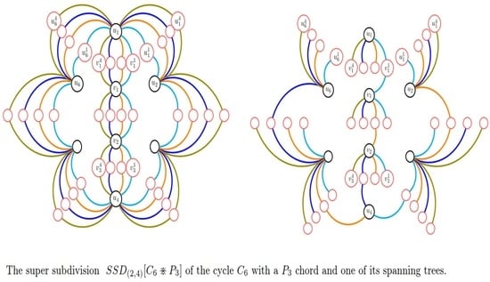
One important algebraic invariant in networks (graphs) nowadays is complexity. This invariant informs us of the total number of acyclic networks in the initial network, which ultimately ensures the accuracy and dependability underlying the network. The super subdivision operation produces a more complex network. In the above work, by using the characteristics of the block matrix, we discovered straightforward and explicit formulas for determining the complexity of the super subdivision of the following graphs: the cycle $C_n$, where $n=3,4,5,6$; the dumbbell graph $D{b}_{m,n}$; the dragon graph $P_m\left(C_n\right)$; the prism graph ${\Pi }_n$, where $n=3,4$; a cycle $C_n$ with a $P_{\frac{n}{2}}$-chord, where $n=4,6$; and the complete graph $K_4$. Finally, the outcomes of our investigation were presented using 3D graphics.

References

1. Bondy, J.A.; Murty, U.S.R. Graph Theory; Springer: New York, NY, USA, 2008. [Google Scholar]
2. Jota, D.-M.; Jäntschi, L. Extending the Characteristic Polynomial for Characterization of C20 Fullerene Congeners. Mathematics 2017, 5, 84. [Google Scholar] [CrossRef] [Green Version]
3. Nikolić, S.; Tolić, I.M.; Trinajstić, N. On the complexity of molecular graphs. Commun. Math. Comput. Chem. 1999, 40, 187–201. [Google Scholar]
4. Nikolić, S.; Trinajstić, N. Complexity of molecules. J. Chem. Int. Commun. Comput. Sci. 2000, 40, 920–926. [Google Scholar]
5. Jane<i>z</i>ˇi<i>c</i>ˇ, D.; Mili<i>c</i>ˇević, A.; Nikolić, S.; Trinajstić, N. Topological Complexity of Molecules. In Encyclopedia of Complexity and Systems Science; Meyers, R., Ed.; Springer: Berlin/Heidelberg, Germany, 2018. [Google Scholar]
6. Gao, Y.; Chen, S.; Tong, J.; Fu, X. Topology-enhanced molecular graph representation for anti-breast cancer drug selection. BMC Bioinform. 2022, 23, 382. [Google Scholar] [CrossRef] [PubMed]
7. Manzoor, S.; Siddiqui, M.K.; Ahmad, S. On entropy measures of molecular graphs using topological indices. Arab. J. Chem. 2020, 13, 6285–6298. [Google Scholar] [CrossRef]
8. Bapat, R.B. Graphs and Matrices; Springer: New York, NY, USA; London, UK, 2010. [Google Scholar]
9. Biggs, N.L. Algebraic Graph Theory, 2nd ed.; Cambridge University Press: Cambridge, UK, 1993. [Google Scholar]
10. Temperley, H.N.V. Graph Theory and Applications; Ellis Horwood Series in Mathematics and its Applications; Ellis Horwood Ltd.: Chichester, UK; Halsted Press: Ultimo, NSW, Australia; John Wiley and Sons, Inc.: New York, NY, USA, 1981. [Google Scholar]
11. Brownaj, T.J.N.; Mallion, R.B.; Pollak, P.; Rothb, A. Some methods for counting the spanning trees in labelled molecular graphs, examined in relation to certain fullerenes. Discret. Appl. Math. 1996, 67, 51–66. [Google Scholar] [CrossRef] [Green Version]
12. Kirby, E.C.; Klein, D.J.; Mallion, R.B.; Paul Pollak, P.; Sachsd, H. A theorem for counting spanning trees in general chemical graphs and its particular application to toroidal fullerenes. Croat. Chem. Acta 2004, 77, 263–278. [Google Scholar]
13. Daoud, S.N. The deletion-contraction method for counting the number of spanning trees of graphs. Eur. Phys. J. Plus 2015, 130, 217. [Google Scholar] [CrossRef]
14. Zhang, Z.; Liu, H.; Wu, B.; Zou, T. Spanning trees in a fractal scale—Free lattice. Phys. Rev. E Stat. Nonlinear Soft Matter 2011, 83, 016116. [Google Scholar] [CrossRef]
15. Teufl, E.; Wagner, S. Determinant identities for Laplace matrices. Linear Algebra Appl. 2010, 432, 441–457. [Google Scholar] [CrossRef] [Green Version]
16. Daoud, S.N.; Saleha, W. Complexity trees of the sequence of some nonahedral graphs generated by triangle. Heliyon 2020, 6, e04786. [Google Scholar] [CrossRef] [PubMed]
17. Zeen El Deen, M.R.; Aboamer, W.A. Complexity of some duplicating networks. IEEE Access 2021, 9, 56736–56756. [Google Scholar] [CrossRef]
18. Zeen El Deen, M.R.; Aboamer, W.A. Complexity of some graphs generated by a square. J. Math. Comput. Sci. 2021, 11, 4248–4283. [Google Scholar]
19. Zeen El Deen, M.R. Enumeration of spanning trees in prisms of some graphs. Proyecciones J. Math. 2023, 42, 339–391. [Google Scholar] [CrossRef]
20. Sun, W.G.; Wang, S.; Zhang, J. Counting spanning trees in a prism and anti-prism graphs. J. Appl. Anal. Comput. 2016, 6, 65–75. [Google Scholar]
21. Shirdareh Haghighi, M.H.; Bibak, K.H. The number of spanning trees in some classes of graphs. Rocky Mt. J. Math. 2012, 42, 1183–1195. [Google Scholar]
22. Liu, J.-B.; Daoud, S.N. The complexity of some classes of pyramid graphs created from a gear graph. Symmetry 2018, 10, 689. [Google Scholar] [CrossRef] [Green Version]
23. Liu, J.-B.; Daoud, S.N. Number of spanning trees in the sequence of some graphs. Complexity 2019, 2019, 4271783. [Google Scholar] [CrossRef] [Green Version]
24. Daoud, S.N. Generating formulas of the number of spanning trees of some special graphs. Eur. Phys. J. Plus 2014, 129, 146. [Google Scholar] [CrossRef]
25. Afzal, H.U.; Javaid, M.; Ovais, A.; Alam, M.N. Computation of the complexity of networks under generalized operations. Complexity 2022, 2022, 6288054. [Google Scholar] [CrossRef]
26. Daoud, S.N.; Mohamed, K. The complexity of Some Families of Cycle-Related Graphs. J. Taibah Univ. Sci. 2017, 11, 205–228. [Google Scholar] [CrossRef] [Green Version]
27. Zhang, F. Matrix Theory; Springer: New York, NY, USA, 2011. [Google Scholar]
28. Marcus, M. A Survey of Matrix Theory and Matrix Inequalities; Unvi. Allyn and Bacon, Inc.: Boston, MA, USA, 1964. [Google Scholar]
29. Gross, D.J.; Saccoman, T.J.; Suffel, L.C. Spanning Tree Results For Graphs Furthermore, Multigraphs: A Matrix-Theoretic Approach; World Scientific Publishing Company: Singapore, 2014. [Google Scholar]
30. Balakrishnan, R.; Ranganathan, K. A Textbook of Graph Theory; Springer Science and Business Media: New York, NY, USA, 2012. [Google Scholar]
Figure 1. Super subdivision S S D ( 2 , t ) ( C 3 ) of the cycle C 3 .
Computation 11 00162 g001
Figure 2. Super subdivision S S D ( 2 , t ) ( D b 4 , 6 ) of the dumbbell graph D b 4 , 6 .
Computation 11 00162 g002
Figure 3. Super subdivision S S D ( 2 , t ) [ P m ( C n ) ] of the dragon graph P m ( C n ) .
Computation 11 00162 g003
Figure 4. Super subdivision S S D ( 2 , t ) ( Π 3 ) of the prism Π 3 .
Computation 11 00162 g004
Figure 5. Super subdivision S S D ( 2 , t ) [ C n P n 2 ] of the cycle C n with a P n 2 chord.
Computation 11 00162 g005
Figure 6. Super subdivision S S D ( 2 , t ) ( K 4 ) of the complete graph K 4 .
Computation 11 00162 g006
Figure 7. Variations in the enumerated complexities of the super subdivision graphs.
Computation 11 00162 g007
Disclaimer/Publisher’s Note: The statements, opinions and data contained in all publications are solely those of the individual author(s) and contributor(s) and not of MDPI and/or the editor(s). MDPI and/or the editor(s) disclaim responsibility for any injury to people or property resulting from any ideas, methods, instructions or products referred to in the content.