The Multi-Maximum and Quasi-Maximum Common Subgraph Problem

Abstract

The Maximum Common Subgraph problem has been long proven NP-hard. Nevertheless, it has countless practical applications, and researchers are still searching for exact solutions and scalable heuristic approaches. Driven by applications in molecular science and cyber-security, we concentrate on the Maximum Common Subgraph among an indefinite number of graphs. We first extend a state-of-the-art branch-and-bound procedure working on two graphs to N graphs. Then, given the high computational cost of this approach, we trade off complexity for accuracy, and we propose a set of heuristics to approximate the exact solution for N graphs. We analyze sequential, parallel multi-core, and parallel-many core (GPU-based) approaches, exploiting several leveraging techniques to decrease the contention among threads, improve the workload balance of the different tasks, reduce the computation time, and increase the final result size. We also present several sorting heuristics to order the vertices of the graphs and the graphs themselves. We compare our algorithms with a state-of-the-art method on publicly available benchmark sets. On graph pairs, we are able to speed up the exact computation by a 2× factor, pruning the search space by more than 60%. On sets of more than two graphs, all exact solutions are extremely time-consuming and of a complex application in many real cases. On the contrary, our heuristics are far less expensive (as they show a lower-bound for the speed up of 10×), have a far better asymptotic complexity (with speed ups up to several orders of magnitude in our experiments), and obtain excellent approximations of the maximal solution with 98.5% of the nodes on average.

1. Introduction

Graphs are incredibly flexible data structures that can represent information through vertices and relations through edges, allowing them to model various phenomena with easily machine-readable structures. We can adopt graphs to represent the relationship between functions in programs, electronic logic devices in synthesis, connections between atoms, and molecules in biology, etc.

Understanding whether two graphs represent the very same object, that is, determining if the two graphs are isomorphic, belongs to the class of NP-complete problems. Scholars are still not sure whether it can be improved, but existing algorithms for solving this problem have exponential complexity [1]. Given two graphs, i.e., $G_1$ and $G_2$, finding the largest graph simultaneously isomorphic to two subgraphs of the given graphs, i.e., $G=MCS(G_1,G_2)$, is even more challenging; it is usually known as the Maximum Common Subgraph (MCS) problem. Nevertheless, this problem is the key step in many applications, such as studying “small worlds” in social networks [2,3], searching the web [4], analyzing biological data [5], classifying large-scale chemical elements [6], and discovering software malwares [7]. Algorithms to find the MCS have been presented in the literature since the 70s [8,9]. Among the most significant approaches, we would like to mention the conversion to the Maximum Common Clique problem [10], the use of constraint programming [11,12] and integer linear programming [13], the extraction of subgraphs guided by a neural network model [14,15], the adoption of reinforcement learning [16], and even multi-engines and GPU-based many-core implementations [17].

This paper proposes a set of algorithms and related heuristics to assess the similarity of a set of graphs and determine how akin each of these graphs is to the whole group. More specifically, we approach the so-called Multi-MCS problem [6,18], i.e., we focus on finding the MCS or a quasi-MCS (one good approximation of the MCS) among N (usually more than two) graphs. Notice that a possible solution to this problem consists of the iterated application of a standard MCS procedure to find the MCS between two graphs, i.e., $MCS(G_1,G_2)$, to a set of N graphs $\{G_1,G_2,\dots ,G_N\}$. Unfortunately, to apply this strategy, we need to fully parenthesize the set of graphs, and the number of possible parenthesizations is exponential in N, i.e., $\Omega \left(2^n\right)$ [19]. Moreover, as each computation $MCS(G_1,G_2)$ potentially has several equivalent solutions, not all parenthesizations deliver the same results. For example, given three graphs $\{G_1,G_2,G_3\}$, computing $MCS(MCS(G_1,G_2),G_3\}$ may give optimal results, whereas computing $MCS(G_1,MCS(G_2,G_3))$ may even deliver an empty solution.

To analyze this problem, we examine the work by McCreesh et al. [20]. This work introduces McSplit, i.e., an efficient branch-and-bound recursive procedure that, given two graphs, $G_1$ and $G_2$, finds one of their MCSs, i.e., $MCS(G_1,G_2)$. The process is based on an intelligent invariant that, given a partial mapping between the vertices of the two graphs, considers a new vertex pair only if the vertices within the pair share the same label. Labels are defined based on the interconnections between vertices. Two vertices only share the same label if they are connected in the same way to all previously mapped nodes. The algorithm also adopts an effective bound prediction that, given the current mapping and the labels of yet-to-map vertices, computes the best MCS size the current recursion path can achieve. In practice, the algorithm prunes all paths of the tree search that are not promising enough; thus, it drastically reduces the search space once a good-enough solution has been found. Unfortunately, even if the constraining effect may be fairly effective, pruning depends on the vertex selection order, which is statically computed at the beginning of the process and is one of the most impairing elements of McSplit. Indeed, the static node-degree heuristic may be sub-optimal, generate many ties on large graphs, and include no strategy to break those ties.

We extend this algorithm in different directions. We first generalize the original approach to handle N graphs simultaneously, i.e., $\{G_1,G_2,\dots ,G_N\}$, and find their MCS, i.e., $MCS(G_1,G_2,\dots ,G_N)$. This algorithm finds maximal common subgraphs, is purely sequential, and extends the recursive process of the original function to generate (and couple) the simple permutations of $(n-1)$ sets of vertices. To maintain the original compactness and efficiency considering N graphs, we revisit the algorithmic invariant, the original bound computation, and the data structure used to store partial information. This algorithm also introduces a domain-sorting heuristic that speeds up the original McSplit procedure on a pair of graphs by more than a 2× factor and delivers even better improvements (up to 10×) when it is applied to more than two graphs.

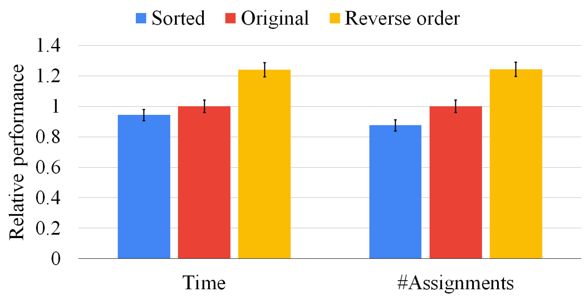
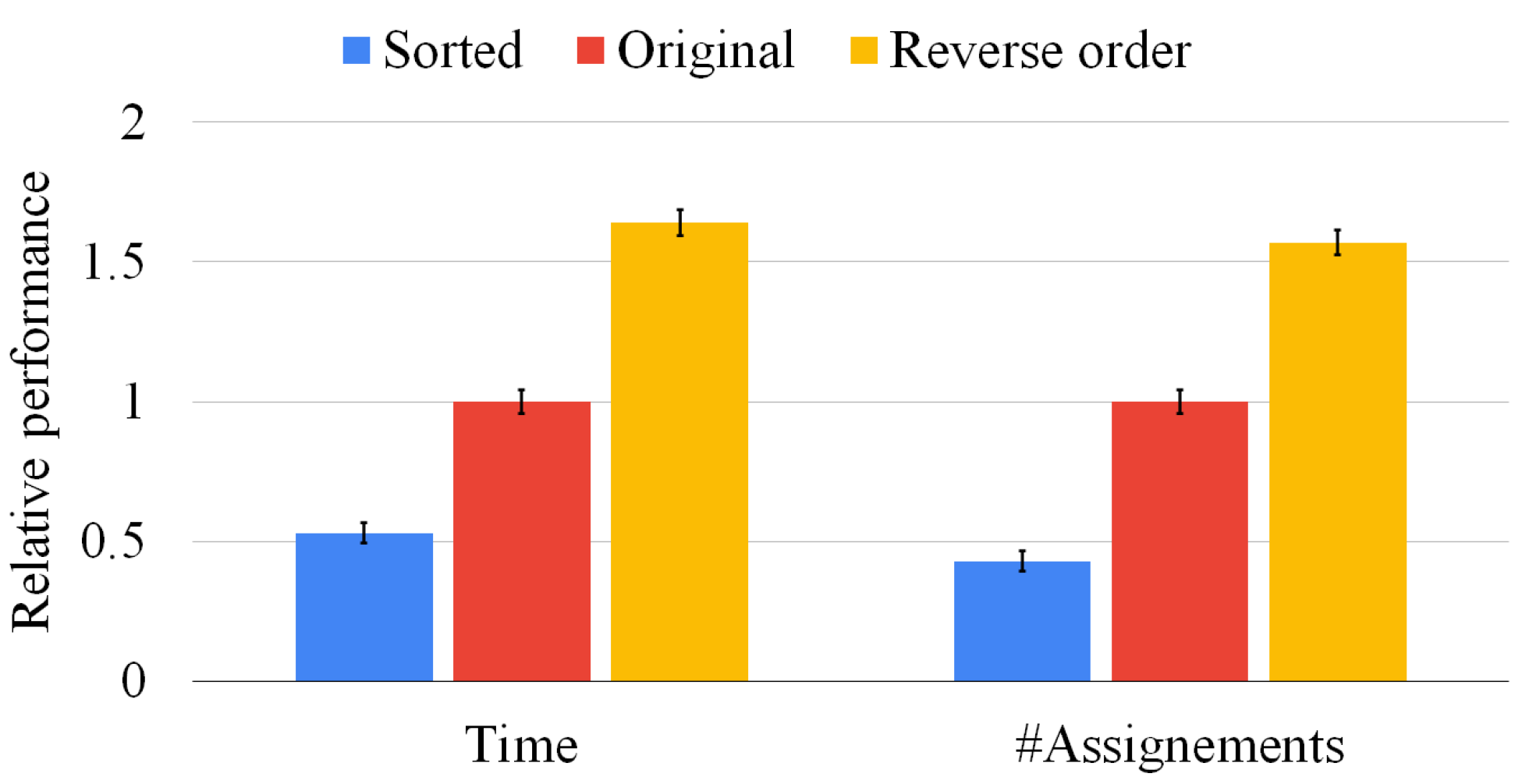
This work is then extended to a parallel multi-core CPU-based procedure to improve its efficiency following the work by Quer et al. [17]. We divide the work into independent tasks and assign these tasks to a thread pool, minimizing the contention among threads, and trying to balance the workload as much as possible, even though the problem remains an intrinsically unbalanced one. Although it is well known that the order in which nodes are processed greatly influences the execution time, we discovered that the order of the graphs also significantly impacts the speed of our procedure (up to over an order of magnitude) without any apparent drawback. As a consequence, we run experiments with different graph sorting heuristics, and we compare these heuristics in terms of computation time and memory used.

Unfortunately, even if the two previous strategies find maximal solutions and sorting heuristics can considerably improve running times, they can only manage a tiny number of medium-size graphs when faced with a timeout of 1000 s. As computation time is the main constraining factor as memory usage is usually not critical in this computation, several applications that produce non-exact solutions requiring only a fraction of the computation time can benefit from algorithms. By trading off computational costs and accuracy, we propose three heuristics to find the closest-possible maximal solution (a quasi-MCS). Moreover, we compare them in complexity, efficiency, and result size. The first strategy, which we call the “waterfall approach”, manipulates the N graphs linearly, such that the MCS of any two graphs, e.g., $MCS(G_1,G_2)$, is compared with the following graph in the list, e.g., $MCS\left(MCS(G_1,G_2),G_3\right)$. The second strategy, which we call the “tree approach”, manipulates the N graphs pair-by-pair in a tree-like fashion, e.g., $MCS\left(MCS(G_1,G_2),MCS(G_3,G_4)\right)$. It is potentially far more parallelizable than the waterfall scheme and can be managed by a distributed approach in case of a high enough number of graphs. At the same time, the quality of its solutions is often limited by the choices performed in the higher nodes of the tree.

Finally, to show the scalability of the tree approach, we call a GPU unit and distribute the branches of the tree-like approach between the two devices leveraging a multi-threading CPU and a many-threading GPU unit. Although the GPU implementation cannot outperform the CPU version in speed, since the implementation deals with an inherently unbalanced problem, the presence of a second device allows us to reduce the execution time when applied to the tree approach.

Our experimental results show the advantages and disadvantages of our procedures and heuristics. We take into consideration the asymptotic complexity and the elapsed time of our tools, and, as some of our strategies sacrifice optimality in favor of applicability, we also consider the result size as an essential metric to compare them. We prove that the heuristic approaches are orders of magnitude faster than the exact original implementations. Even if they cannot guarantee the maximality of their solution, we prove that their precision loss is shallow once the proper countermeasures are implemented.

To sum up, this paper presents the following contributions:

• An extension of a state-of-the-art MCS algorithm to solve the Multi-MCS problem adopting both a sequential and a parallel multi-threaded approach. These solutions manipulate the N-graphs within a single branch-and-bound procedure.
• A revisitation of the previous multi-threaded approach to solving the Multi-quasi-MCS problem, trading-off computation time and accuracy. In these cases, our solutions deal with the N-graphs on a graph-pair basis with different logic schemes.
• A mixed parallel multi-core (CPU-based) and many-core (GPU-based) extension of the previous algorithms for a non-exhaustive search to further reduce the computational time distributing the effort on different computational units.
• An analysis of sorting heuristics applicable to vertex bidomains, graph pairs, and set of graphs able to significantly improve the solution time with a minimal increase in the algorithmic complexity.

As far as we know, this is the first work facing the Multi-MCS (and the Multi-quasi-MCS) problem consistently, presenting both exact (maximal) and approximated (quasi-maximal) algorithms to solve it.

The paper is organized as follows. Section 2 reports some background on multi-graph isomorphism and introduces McSplit. Section 3 describes our sequential and parallel multi-core McSplit extensions to handle the Multi-MCS problem. Section 4 shows our implementations of the Multi-quasi-MCS problem tackled as a linear (sequential) or tree (parallel) series of MCS searches. Section 5 introduces the proposed sorting heuristics. Section 6 reports our findings in terms of result size, computation time, and memory used. Section 7 draws some conclusions and provides some hints on possible further developments.

2. Background and Related Works

2.1. Graphs and Notation

In our work, we consider unweighted, directed, or undirected graphs $G=(V,E)$, where V is a finite set of vertices and E is a binary relation on V representing a finite set of edges. We indicate the number of vertices $v\in V$ with n, or $\left|V\right|$, and the number of edges $e\in E$ with m, or $\left|E\right|$. For undirected graphs, E consists of unordered pairs of vertices rather than ordered pairs. We consider graphs as unlabeled even if labels are reported in our examples to describe the logic of our algorithms.

The Maximum Common Subgraph (MCS) problem has received multiple definitions, depending on what we try to maximize. The two main versions of this problem aim to find the “maximum number of nodes” or the “maximum number of edges” that the subgraph must preserve. We mainly refer to the former case in this paper, i.e., given a pair of graphs $G_1$ and $G_2$, the $MCS(G_1,G_2)$ is a graph containing the maximum number of vertices while still being isomorphic to an induced subgraph of both $G_1$ and $G_2$. Figure 1 shows a graphical example of two graphs and some possible MCSs. Notice again that node labels, i.e., $\{1,2,3,4,5\}$ and $\{a,b,c,d,f\}$, are reported to identify all vertices and their pairing uniquely but are of no use to match vertices.

In this paper, we often consider a set of graphs $\{G_1,G_2,\dots ,G_N\}$. In this case, we indicate the number of vertices and edges of $G_i$ with $n_i$ and $m_i$, respectively. N indicates the number of graphs in the set. The previous definition of the MCS can be easily extended to a set of N graphs.

2.2. The McSplit Procedure

McSplit [20] is a branch-and-bound procedure that finds the MCS of a pair of graphs using a depth-first search. To illustrate its main ideas, we apply McSplit to the two graphs, $G_1$ and $G_2$, represented in Figure 2a,b.

Starting from an empty mapping M between the vertices of $G_1$ and $G_2$, McSplit adds a vertex pair to M at each recursion level. During the first recursion step, let us suppose the procedure selects vertex 1 in $G_1$ and vertex b in $G_2$; that is, $M=\{1,a\}$. After that, the function labels each unmatched vertex in $G_1$ according to whether it is adjacent to vertex 1, and it labels each unmatched vertex in $G_2$ according to whether it is adjacent to vertex a. Adjacent vertices have a label of 1, and non-adjacent vertices have a label of 0. Table 1a shows these labels just before the second recursion level.

Table 1. Labels (L) on the non-mapped vertices (v) of $G_1$ and $G_2$.

a  M = {1,a}							b  M = {13,ab}							c  M = {132,abc}
${\mathit{G}}_1$		${\mathit{G}}_2$					${\mathit{G}}_1$		${\mathit{G}}_2$					${\mathit{G}}_1$		${\mathit{G}}_2$
$\mathit{v}$	$\mathit{L}$	$\mathit{v}$	$\mathit{L}$				$\mathit{v}$	$\mathit{L}$	$\mathit{v}$	$\mathit{L}$				$\mathit{v}$	$\mathit{L}$	$\mathit{v}$	$\mathit{L}$
2	1	b	1				2	11	c	11				4	110	d	111
3	1	c	1				4	11	d	11
4	1	d	1

Table 1. Labels (L) on the non-mapped vertices (v) of $G_1$ and $G_2$.

a  M = {1,a}							b  M = {13,ab}							c  M = {132,abc}
${\mathit{G}}_1$		${\mathit{G}}_2$					${\mathit{G}}_1$		${\mathit{G}}_2$					${\mathit{G}}_1$		${\mathit{G}}_2$
$\mathit{v}$	$\mathit{L}$	$\mathit{v}$	$\mathit{L}$				$\mathit{v}$	$\mathit{L}$	$\mathit{v}$	$\mathit{L}$				$\mathit{v}$	$\mathit{L}$	$\mathit{v}$	$\mathit{L}$
2	1	b	1				2	11	c	11				4	110	d	111
3	1	c	1				4	11	d	11
4	1	d	1

At this point, the procedure recurs to extend M with a new pair in which each vertex shares the same label. If during the second recursion step, McSplit extends M with pair 2 and c, it obtains the new mapping $M=\{12,ab\}$ and the new label set is represented in Table 1b. The third step consists of extending M with 3 and a, which is, at this point, the only remaining possibility. The process obtains $M=\{123,abc\}$ and the label set of Table 1c. The last two vertices 4 and d cannot be inserted in M because they have different labels. Then, the recursive procedure backtracks, searching for another (possibly longer) match M.

Notice that within a class of vertices sharing the same label, i.e., belonging to the same domain, McSplit heuristically gives the highest priority to the nodes with the highest degree. Moreover, to reduce the computation effort, McSplit computes a bound to prune the space search and avoid exhaustive searches effectively. In practice, while parsing a branch, McSplit evaluates the following bound:

$$bound=\left|M\right|+\sum _{l\in L}min\left(\right|\{v\in G_1\backslash M:label\left(v\right)=l\}|,|\{v\in G_2\backslash M:label\left(v\right)=l\}\left|\right)$$

(1)

where $\left|M\right|$ is the cardinality of the greatest mapping found so far and L is the actual set of labels. If the bound is smaller than the size of the current mapping, there is no reason to follow that path, as it is not possible to find a matching set longer than the current one along it. In this case, the algorithm prunes the branch of the decision tree, drastically reducing the computation effort, and it moves to the next tree path.

2.3. Related Works

MCS problems are common in many fields and have been widely studied [11,12,21,22,23,24,25,26,27]. For that reason, we discuss only the works closest to ours and dealing with branch and bound, constraint programming methods, and the Multi-MCS problem.

McGregor [21] proposes a branch and bound approach in which each node of a searching tree is paired with two graph nodes. To make the visit efficient, when he visits the tree, he prunes branches that cannot improve the current best solution. Vismara et al. [11] associate each vertex of the first graph with each viable vertex of the second graph using a constraint programming approach. This approach was later improved upon by Ndiaye and Solnon [24]. McCreesh et al., in a series of publications [12,20,28], propose to run a similar constraint programming approach in parallel on multiple cores, significantly reducing the time needed to reach a solution.

The Multi-MCS problem has been left largely unexplored because of its overwhelming complexity. However, a few researchers have proposed methods to approach it, even if none compare the approach with an exact solution. Hariharan et al. [18] discuss how the approaches that try to solve the Multi-MCS problem by finding the MCS between pairs of graphs struggle to find large MCS between multiple graphs in a timely manner. Moreover, they show that many of the heuristics that produce good results on pair of graphs are either non-applicable or ineffective when extended to multiple graphs. As a consequence, they propose an approach based on computing the correspondence graphs between the main graph, referred to as pivot, and all other graphs. Then, they compute the maximum cliques on each of the correspondence to find all connected substructures shared by graph pairs. Finally, they compute the intersection among all substructures and return this intersection as the MCS between the N graphs. Following this work, Dalke et al. [6] proposed FMCS, a heuristic approach based on subgraph enumeration and isomorphism. While exact strategies use algorithms that are computationally very expensive, their approach, although heuristic, produces results competitive with exact methods.

Larsen et al. [29] focused on the maximum common edge subgraph variant. They proposed a heuristic method to optimize the conservation of the maximum number of edges in a set of graphs. Their method relies on repeated local searches for an MCS interleaved with a perturbation step to leave possible local maxima and cover a greater variety of pairings. Their local search is based on a fitness function that identifies the sets of nodes with a good similarity and quickly converges to the final solution. Although the code for this study is freely available, we do not report any direct comparison with it since it maximizes the number of edges in the solution and not the number of nodes. As a consequence, their algorithm prefers smaller but denser solutions to larger but sparser subgraphs.

3. The Multi-MCS Approach

While the MCS problem has multiple applications in different scenarios, Multi-MCS has been mainly studied in molecular science and cyber-security due to its extremely high costs. Surely, more efficient algorithms would push forward its applicability in other research sectors. For this reason, in this section, we present two algorithms extending McSplit [20] to directly consider a set of N graphs $\{G_1,G_2,\dots ,G_N\}$. The first version is purely sequential, whereas the second one is its multi-core CPU-based parallel variation. The efficiency of both versions strongly depends on the graph order. As a consequence, we dedicate the last subsection of this part to describing our sorting heuristics.

3.1. The Sequential Approach

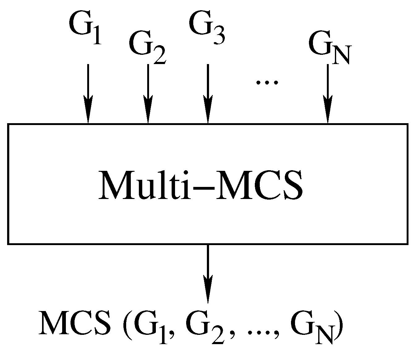
Our first contribution is to rewrite the McSplit algorithm in a sequential form and in such a way that it can handle any number of graphs. A single call to our branch-and-bound procedure Multi-MCS ($G_1,G_2,\dots ,G_N$) computes the MCS of N graphs $\{G_1,G_2,\dots ,G_N\}$. Figure 3 illustrates the inputs and outputs of the function, and Algorithm 1 reports its pseudo-code.

To obtain an efficient implementation, we modify a few core steps of the original algorithms, maintaining the main perks of the logic flow together with its overall memory and time efficiency.

Algorithm 1 The sequential Multi-MCS function: A unique recursive branch-and-bound procedure that given N graphs $\{G_1,G_2,\dots ,G_N\}$ and computes $MCS\{G_1,G_2,\dots ,G_N\}$

1: Multi-MCS ($\{G_1,G_2,\dots ,G_N\}$) 2: $C=S=\varnothing$ 3: level = 0 4: domains = initial domains 5: selectFirstNode ($\{G_1,G_2,\dots ,G_N\}$, C, S, level, domains) 6: return S

7: selectFirstNode ($\{G_1,G_2,\dots ,G_N\}$, C, S, level, domains) 8: if ($\left|C\right|>\left|S\right|$) then 9:    $S=C$ 10: end if 11: while $domains\ne \varnothing$do 12:    bound = computeBound ($\{G_1,G_2,\dots ,G_N\}$, C) 13:    if (bound ≤$\left|S\right|$) then 14:    return 15:    end if 16:    domain = selectLabelClass ($\{G_1,G_2,\dots ,G_N\}$, domains) 17:    v = selectVertex (domain) 18:    $G_1=G_1\backslash v$ 19:    $C=C\cup v$ 20:    selectNextNode ($\{G_1,G_2,\dots ,G_N\}$, C, S, level + 1, domains, domain) 21:    $C=C\backslash v$ 22: end while

23: selectNextNode ($\{G_1,G_2,\dots ,G_N\}$, C, S, level, domains, domain) 24: $H=G_{(level\%N)}$ 25: for all u ∈ domain[H] do 26:    $H=H\backslash u$ 27:    $C=C\cup u$ 28:    if ((level % N) == N − 1) then 29:    new_domains = filterDomains ($\{G_1,G_2,\dots ,G_N\}$, C, domains) 30:    // Select new domain on first graph 31:    selectFirstNode ($\{G_1,G_2,\dots ,G_N\}$, C, S, level + 1, new_domains) 32:    else 33:    // Select node from another graph 34:    selectNextNode ($\{G_1,G_2,\dots ,G_N\}$, C, S, level + 1, domains, domain) 35:    end if 36:    $H=H\cup u$ 37:    $C=C\backslash u$ 38: end for

The algorithm selects a node of the first graph and a node of the second graph so that each edge and non-edge toward nodes belonging to the current solution is preserved. After selecting each new node pair, the algorithm divides the “remaining” nodes into sub-sets. These sub-sets are called “domains” in the original formulation, are created by function filterDomains, and group nodes sharing the same set of adjacency and non-adjacency toward the nodes in the current solution. Two domains belonging to different graphs that share the same adjacency rules to nodes in their respective graphs are then paired in what is called a “bidomain”. The nodes within a bidomain are thus compatible and can be matched. For each bidomain, the size of the smallest domain is used by function computeBound to compute how many nodes can still be added to the solution along that specific path, pruning the search whenever possible.

In our implementation, to handle more than two graphs and maintain the original algorithmic efficiency, we revise both the logic and the data structure of the algorithm. Our Multi-MCS procedure begins by initializing its variables C (representing the current solution), S (the best solution found) with an empty solution, and the variable level (representing the number of nodes already selected) to zero. Finally, it assigns an initial value to the variable domains, which depends on the nature of the graph: when the graph has no label, all nodes in the graph belong to a single domain; otherwise, the initial number of domains is equal to the number of different labels. Then, the algorithm performs the selection of a node from the first and a node from the second graph in two steps. Function selectFirstNode, called in line 4, selects the multi-domain (a bidomain extended to multiple graphs) from which the nodes is chosen to be added to our solution, and it selects the node of the first graph. Function selectNextNode, called in line 20, works on the same multi-domain until it has selected a node from each of the other graphs.

The function selectFirstNode first updates the current best solution (lines 8–10). Then, it computes the current bound using the function computeBound (line 12). If the bound proves that we will not be able to improve the current best solution, we return (line 14) and try to select a different set of nodes in order to reach a better solution. If we can still improve the current best solution, we then choose the multi-domain from which to select the vertices. This step is performed by function selectLabelClass (line 16). While different node sorting heuristics can improve the performance of the algorithm, we followed the same logic used in the McSplit algorithm, preferring a fail-first approach. This method entails that the function always selects the smallest multi-domain to quickly check all possible matchings, and therefore, it allows us to definitely remove them from the current branch of execution. From the selected multi-domain, we select the node with the highest number of neighboring nodes (another heuristic borrowed from McSplit), we add it to our current solution, and we remove it from the list of non-selected nodes. In line 20, we call selectNextNode to proceed to the other graphs. When all possible matchings have been checked, we remove the selected node from the solution and try to improve on the current one by avoiding the selection of the node just discarded. The standard C-like implementation proceeds with dynamically allocated data structures for the domains and bidomains. Nevertheless, in some cases, dynamic allocation may drastically influence performance. As a consequence, in Section 3.2, we also discuss the possibility of adopting pre-allocated (static) memory to reduce overheads, even if this solution somehow limits the flexibility of the algorithm.

The function, selectNextNode, is a much simpler function. It works on the already chosen multi-domain and selects a vertex from each of the remaining graphs (i.e., $\{G_2,\dots ,G_N\}$)—more specifically, from the domains belonging to the same multi-domain. In this function, we refer to the set of all graphs $\{G_1,\dots ,G_N\}$ with G. Since, as we have already discussed, the vertices belonging to the same multi-domain can be paired without producing conflicts, this is a pretty straightforward task. Once again, the order of selection is unsophisticated, as we chose the vertices by sorting them by the number of respective adjacency. Once we have selected a node from each graph, we call the function filterDomains (line 29) to update the domains previously computed, and we recur on the next multi-domain (line 31).

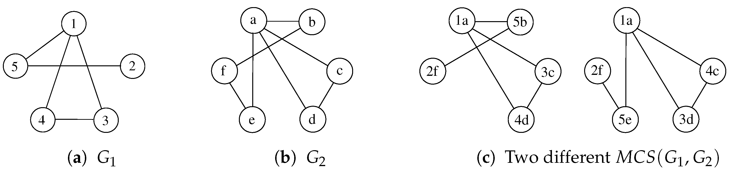
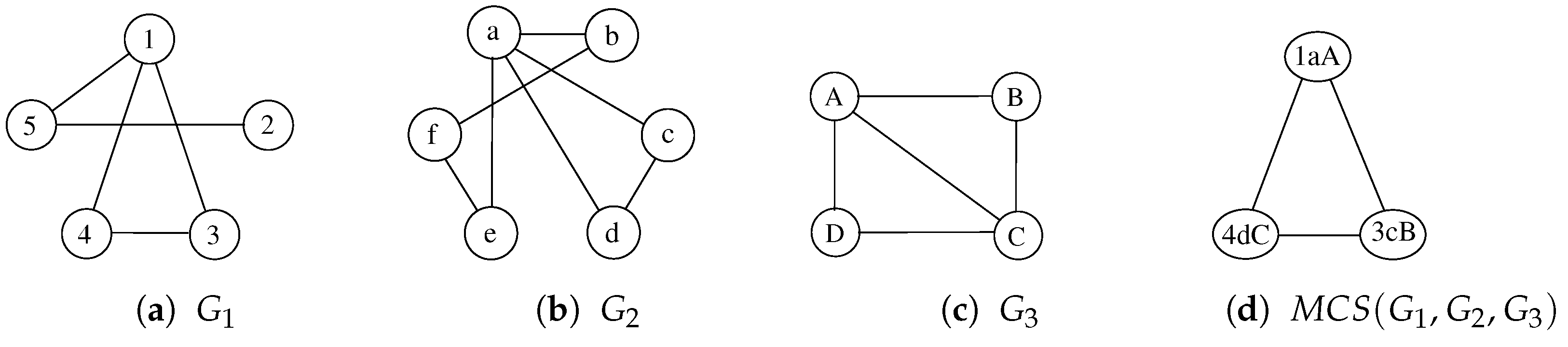
To better describe our procedure, following Figure 2 and Table 1, we illustrate a possible sequence of node selection and node labeling with three graphs in Figure 4 and Table 2. For the sake of simplicity, Table 2 does not represent the actual execution steps performed by the algorithm since a correct execution of the procedure finds multiple non-maximal solutions from which it has to backtrack before gathering the MCS. As a consequence, we select a sequence of three steps that lead to one of the admissible MCS, showing the node selection process and the evolution of the labels. The example starts by selecting the nodes 1, a, and A from graphs $G_1$, $G_2$, and $G_3$, respectively. Starting from this partial solution, the function separates the other nodes into two domains, depending on their adjacency with the selected nodes. During the second step, the procedure selects the nodes 3, c, and B from the adjacent domain, creating three new domains. Finally, during the third step, function Multi-MCS selects the nodes 4, d, and C. None of the resulting domains appears in all three graphs; thus, the algorithm backtracks to look for a better solution.

Table 2. Labels on the non-mapped vertices of $G_1$, $G_2$ and $G_3$.

a  M = {1,a,A}							b  M = {13,ac,AB}									c  M = {134,acd,ABC}
${\mathit{G}}_1$		${\mathit{G}}_2$		${\mathit{G}}_3$			${\mathit{G}}_1$		${\mathit{G}}_2$		${\mathit{G}}_3$					${\mathit{G}}_1$		${\mathit{G}}_2$		${\mathit{G}}_3$
$\mathit{v}$	$\mathit{L}$	$\mathit{v}$	$\mathit{L}$	$\mathit{v}$	$\mathit{L}$		$\mathit{v}$	$\mathit{L}$	$\mathit{v}$	$\mathit{L}$	$\mathit{v}$	$\mathit{L}$				$\mathit{v}$	$\mathit{L}$	$\mathit{v}$	$\mathit{L}$	$\mathit{v}$	$\mathit{L}$
2	0	b	1	B	1		2	00	b	10	C	11				2	000	b	100	D	001
3	1	c	1	C	1		4	11	d	11	D	00				5	100	e	100
4	1	d	1	D	0		5	10	e	10								f	00
5	1	e	1						f	000
		f	0

Table 2. Labels on the non-mapped vertices of $G_1$, $G_2$ and $G_3$.

a  M = {1,a,A}							b  M = {13,ac,AB}									c  M = {134,acd,ABC}
${\mathit{G}}_1$		${\mathit{G}}_2$		${\mathit{G}}_3$			${\mathit{G}}_1$		${\mathit{G}}_2$		${\mathit{G}}_3$					${\mathit{G}}_1$		${\mathit{G}}_2$		${\mathit{G}}_3$
$\mathit{v}$	$\mathit{L}$	$\mathit{v}$	$\mathit{L}$	$\mathit{v}$	$\mathit{L}$		$\mathit{v}$	$\mathit{L}$	$\mathit{v}$	$\mathit{L}$	$\mathit{v}$	$\mathit{L}$				$\mathit{v}$	$\mathit{L}$	$\mathit{v}$	$\mathit{L}$	$\mathit{v}$	$\mathit{L}$
2	0	b	1	B	1		2	00	b	10	C	11				2	000	b	100	D	001
3	1	c	1	C	1		4	11	d	11	D	00				5	100	e	100
4	1	d	1	D	0		5	10	e	10								f	00
5	1	e	1						f	000
		f	0

3.2. The Parallel Approach

To improve the efficiency of Algorithm 1 and following Quer et al. [17], we modified the previous procedure to handle tasks in parallel. Algorithm 2 reports the new pseudo-code. Functions selectFirstNode and selectNextNode are not reported as they are identical to the ones illustrated in Algorithm 1.

Algorithm 2 The parallel many-core CPU-based Multi-MCS Function: A unique recursive function that, given N graphs $\{G_1,G_2,\dots ,G_N\}$, computes $MCS\{G_1,G_2,\dots ,G_N\}$ running several tasks

1: Multi-MCS ($\{G_1,G_2,\dots ,G_N\}$, C, S, level, domain) 2: if (level % N) == 0 then 3:    if ($level\le PART\_LEVEL$) then 4:    $task$ = { $\{G_1,G_2,\dots ,G_N\}$, C, S, level } 5:    enqueue (selectFirstNode, $task$) 6:    else 7:    selectFirstNode ($\{G_1,G_2,\dots ,G_N\}$, C, S, level) 8:    end if 9: else 10:    selectNextNode ($\{G_1,G_2,\dots ,G_N\}$, C, S, level, domain) 11: end if

The parallelization of the algorithm is achieved by dividing the workload among a pool of threads. Each thread waits on a synchronized queue which is filled with new tasks as represented in line 5 of the pseudo-code. Two objects are loaded into the queue: the pointer to the function to be executed, i.e., function selectFirstNode; and the data block needed for the execution, i.e., the variable $task$. Once an item has been placed in the queue, the first available (free) thread will start working independently from the others, thus allowing a high level of parallelism. Since synchronization among threads often requires a significant amount of time, we only divide the work between various threads if the variable $level$ is less than a threshold ($PART\_LEVEL$) whose value can be selected experimentally. After this level, the rest of the execution takes place similarly to Algorithm 2, so that all threads are independent from each other.

The main problem of this function is due to the use of variable-sized arrays. A detailed code implementation showed that the compiler could not optimize the memory allocation of the new data structures, and this inefficiency resulted in a significant slowdown of the program when compared to the original implementation on graph pairs. To address this issue, we then implemented a second version of the algorithm where the main data structures were allocated statically of an oversize dimension. This second version showed significant speed ups compared to the original one both in the MCS (where it has achieved the performances of the original function) and in the multi-MCS problem.

3.3. Conclusions on Exact Multi-MCS Approaches

To understand the complexity of the Multi-MCS problem, we borrow some definitions from the world of combinatorics. When we consider two graphs, $G_1$ and $G_2$, excluding any possible optimization, the number of possible matches between the nodes of $G_1$ (with $n_1$ nodes) and the nodes of $G_2$ (with $n_2$ nodes) equals the number of injective functions from the set of vertices $V_1$ and the set of vertices $V_2$. If we call i the number of elements of the smaller set that we will not pair with one of the second set, it is sufficient to compute the following to obtain the number of these functions:

$$\begin{array}{ccc}\hfill (n_2\ge n_1)& \to & {\sum }_{i=0}^{n_1-1}\left\{\frac{n_2!}{[n_2-(n_1-i)]!}·\frac{n_1!}{(n_1-i)!i!}\right\}\hfill \end{array}$$

(2)

To understand the previous equation, let us start by focusing separately on the two fractions. The first element of the equation represents the number of permutations of $(n_1-i)$ elements of the $n_2$ elements of the second set, whereas the second fraction represents the number of combinations of the $(n_1-i)$ elements of the $n_1$ elements of the first set. The permutations represent, given a set of $(n_1-i)$ elements of the first graph, all possible distinct pairings one can achieve using the $n_2$ elements of the second graph. The combinations represent all possible distinct sets of $(n_1-i)$ elements that we can select from the first graph. To conclude, we need to compute the summation that goes from zero (when we take all the elements of the first graph) to $n_1$, when we do not take any elements. We consider only the empty set.

When we add a third graph, or a third set, the equation remains largely unchanged, even if we need to add a new factor:

$$\begin{array}{ccc}\hfill (n_3\ge n_1,n_2\ge n_1)& \to & {\sum }_{i=0}^{n_1-1}\left\{\frac{n_3!}{[n_3-(n_1-i)]!}·\frac{n_2!}{[n_2-(n_1-i)]!}·\frac{n_1!}{(n_1-i)!i!}\right\}\hfill \end{array}$$

(3)

Although the algorithm is extremely efficient, it cannot deal with the complexity of the Multi-MCS problem in a timely manner when comparing even small graphs in a large enough number. For this reason, in the following section, we discuss the Multi-quasi-MCS problem, introducing non-exact methodologies able to solve the problem by visiting only a fraction of the search tree. Since the MCS problem is difficult to approximate with algorithms with lower complexity than those able to compute an exact solution, our approach inevitably fails to find the MCS, but we discuss features added to the code to lower the probability of such a problem presenting itself.

4. The Multi-Quasi-MCS Approach

Due to the extremely long time required to solve the multi-MCS problem, we decided to trade off time and maximality. Section 4.1 illustrates a first approach considering the sequence of all graphs in pairs. Section 4.2 shows an attempt to improve the maximality of the previous approach without increasing the complexity of the algorithm too much. Section 4.3 illustrates an alternative approach that allows a greater degree of parallelization.

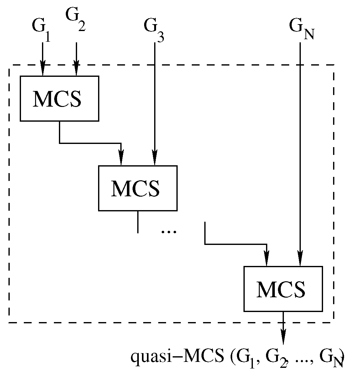
4.1. The Waterfall Approach

Our first Multi-quasi-MCS approach follows the logic illustrated in Figure 5, and Algorithm 3 reports its pseudo-code. Due to the order in which the graphs are considered, we refer to this method as the “waterfall” approach.

Algorithm 3 The trivial multi-graph, i.e., Multi-quasi-MCS $\left(\{G_1,G_2,G_3,\dots ,G_N\}\right)$, branch-and-bound procedure

1: Multi-quasi-MCS ($\{G_1,G_2,G_3,\dots ,G_N\}$) 2: sol = Solve ($G_1$, $G_2$) 3: for all g in $\{G_3,G_4,\dots ,G_N\}$ do 4:    $sol$ = Solve ($sol$, g) 5: end for 6: return $sol$

The waterfall approach consists of finding the MCS between two graphs through the original McSplit algorithm. Then, the computed subgraph is used as a new input to solve the MCS problem with the next graph.

In our implementation (Algorithm 3, lines 2 and 4), we adopt a parallel version of McSplit (for pairs of graphs) to implement the function Solve. However, from a high-level point of view, the approach is structurally sequential as it manipulates a graph pair at each stage, and parallelism is restricted to every single call to the Solve function. Indeed, we present an approach that increases the level of parallelism in Section 4.3. As a final observation, please notice that it is possible to implement several minor variations of Algorithm 3 by changing the order in which the graphs are considered. For example, we can easily insert graphs in a priority queue (i.e., a maximum or minimum heap) using the size of the graphs as the priority. In this case, we can extract two graphs from the queue just before calling the function Solve in line 4 and insert the result, sol, in the same queue after this call. The main difference with the original algorithm is the design of the data structure necessary to store intermediate solutions and the logic used to store in it all intermediate results.

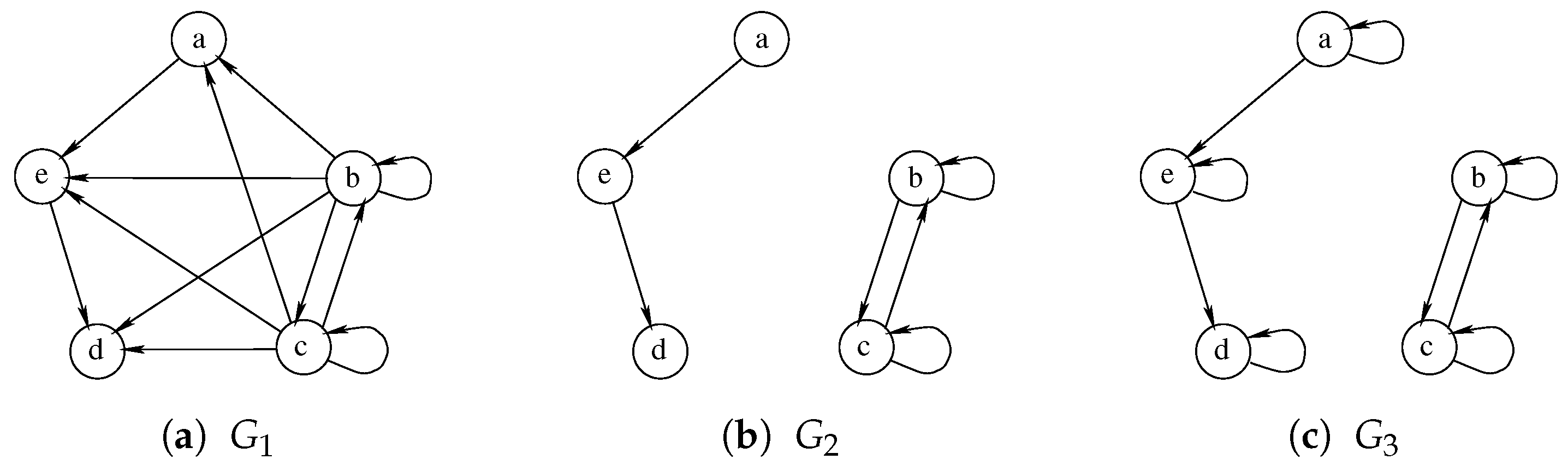
Albeit being very simple, Hariharan et al. [18] prove that a similar approach may not be able to guarantee the quality of the solution and could even return a zero-sized solution where better ones exist. Furthermore, the size of the final solution is strictly dependent on the order in which the graphs are considered, making some ordering strictly better than others. For example, Figure 6 illustrates an example with three graphs on which, using the order $\{G_1,G_2,G_3\}$, the waterfall approach returns an empty solution. The algorithm correctly identifies the MCS between graph $G_1$ and $G_2$, selecting the nodes a, d, and e on both of them. Unfortunately, the MCS between this solution and $G_3$ is an empty graph as all nodes of $G_2$ have self-loops, while none of the nodes of the intermediate solution share this characteristic. On the contrary, the exact approach, by analyzing all the graphs simultaneously, can select the nodes b and c as a Multi-MCS of the graphs $\{G_1,G_2,G_3\}$.

As previously mentioned, considering the graphs in different orders would allow us to obtain different and possibly better solutions. If we solved the triplet of graphs in reverse order $\{G_3,G_2,G_1\}$, the solution between $G_3$ and $G_2$ would return nodes b and c, which possess both the self-loop and a double edge. Then, calculating the MCS between this solution and $G_1$, both nodes b and c would be preserved, leading us to the exact solution.

Despite the above problems, the complexity of this solution is orders of magnitude smaller than the one of Section 3. Let us designate the number of nodes of $G_1$, $G_2$ and $G_3$ to be $n_1$, $n_2$ and $n_3$, respectively; let us call $\alpha$ the size of the MCS of the first two graphs. Then, the complexity of solving three graphs can be evaluated as

$$\begin{array}{ccc}\hfill (n_3\ge n_2\ge n_1)& \to & {\sum }_{i=0}^{n_1-1}\left\{\frac{n_2!}{[n_2-(n_1-i)]!}·\frac{n_1!}{(n_1-i)!i!}\right\}+{\sum }_{i=0}^{\alpha -1}\left\{\frac{n_3!}{[n_3-(\alpha -i)]!}·\frac{\alpha !}{(\alpha -i)!i!}\right\}\hfill \end{array}$$

(4)

Which amounts to a significant improvement over Equation (3), where the two summations were multiplied by each other.

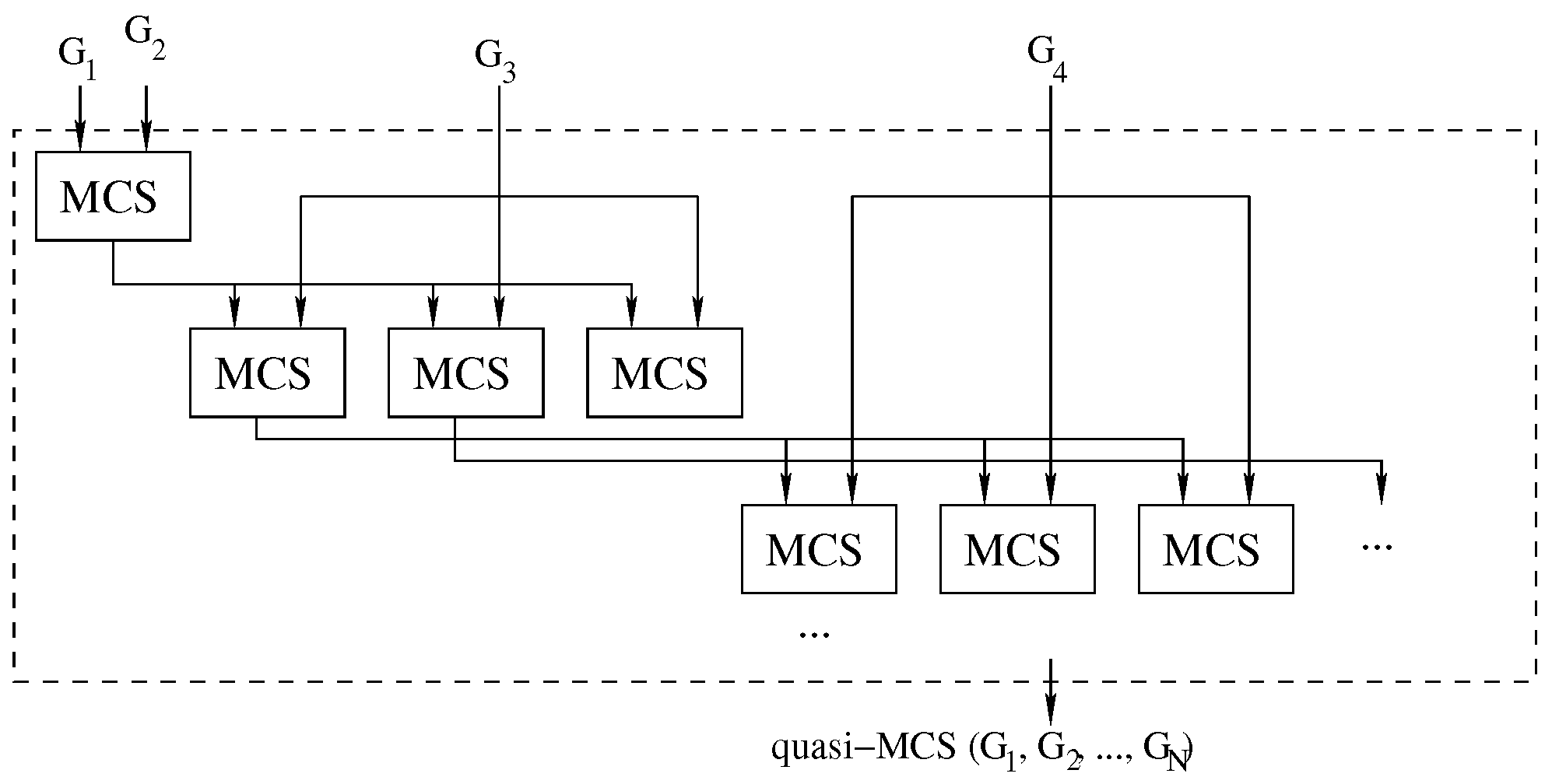
4.2. The Multi-Way Waterfall Approach

To improve the quality of the solutions delivered by the waterfall approach, we modified it using the logic illustrated in Figure 7.

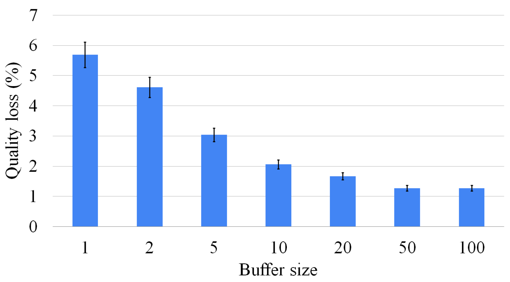
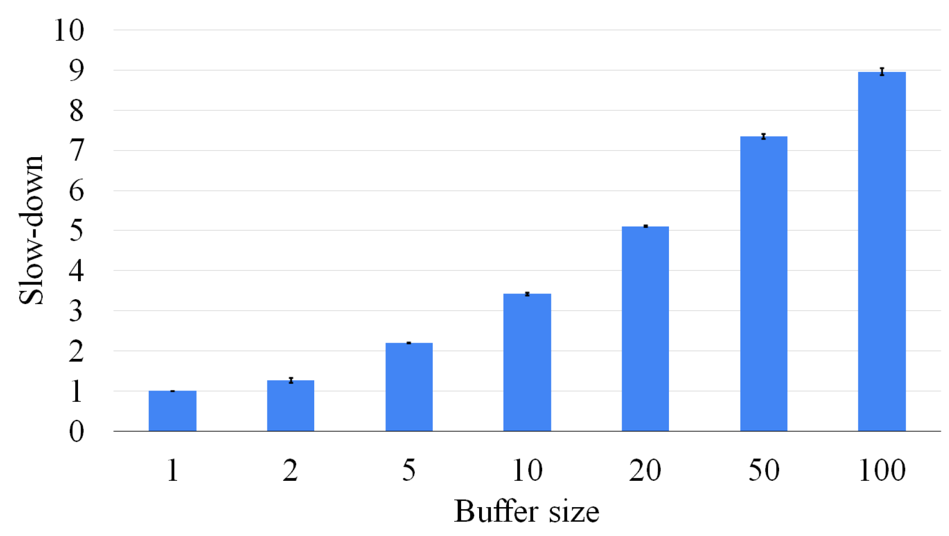
To reduce the impact of selecting an “unfortunate” MCS solution, which means that using it as input for future MCS searches would inevitably lead to a “small” final common subgraph, we have opted to store an arbitrary number of solutions at each intermediate step. To avoid an exponential tree-like explosion in the number of considered solutions, we heuristically set this number to a constant value $\widehat{N}$. As a consequence, in each phase of the search, we consider the $\widehat{N}$ most promising solutions collected in the previous step, and we generate $\widehat{N}$ new best solutions for the next stage. The process is repeated until no graphs are left, as illustrated in Figure 7.

One of the problems with the multi-way waterfall approach is that several intermediate solutions are isomorphic, making the entire process somehow redundant. To rectify this problem, for each MCS call, we insert a post-processing step checking for each new solution whether the selected nodes differ with respect to the ones chosen for the previous solution. This process flow avoids the simplest case of isomorphism. Although verifying the node selection is a very unreliable and approximate way of checking whether two solutions are isomorphic, it is extremely fast, does not slow down the execution, and improves the final result’s size in many cases. Indeed, in Section 6, we prove that over hundreds of executions, the size difference between the MCS and our solution is really small, usually consisting of only one vertex and occasionally two on MCS of the order of 10–25 vertices. Considering all experiments, the average error is under one vertex.

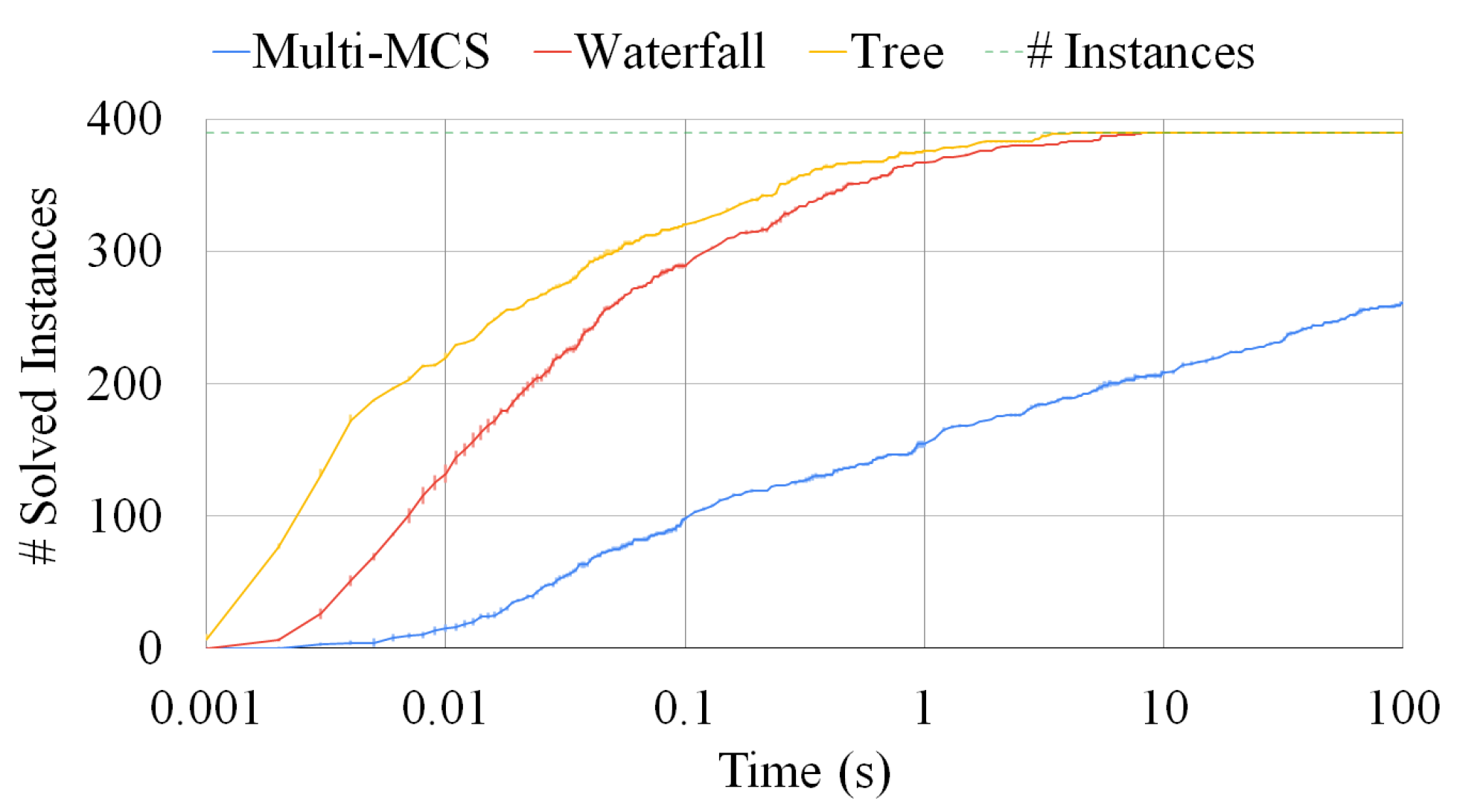
If we increase the number of intermediate solutions considered, the average error decreases, even if the reduction is limited if we consider more than five intermediate solutions. Overall, the multi-way waterfall approach is not only orders of magnitude faster than the exact approach, but the complexity of solving harder problems is slow-growing. For example, there are cases in which the exact approach cannot find a solution after 1000 s, and it returns only a partial solution, whereas this approach finds a larger solution within hundredths of a second.

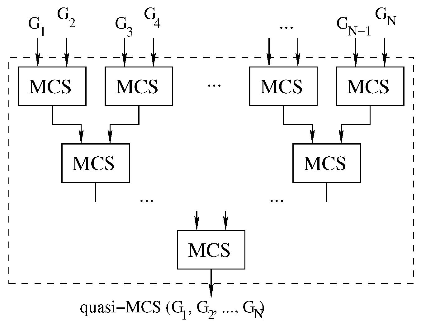
4.3. The Tree Approach

To further increase the parallelism of the approach, it is possible to consider pairs of graphs in a tree-like fashion until the final solution is discovered, as shown in Figure 8.

Algorithm 4 shows a simple implementation of this approach. Due to the order in which the process is structured, we will refer to this implementation as the “tree” approach.

Algorithm 4 The tree approach: increasing the parallelism of the waterfall strategy

1: Multi-quasi-MCS ($\{G_1,G_2,G_3,\dots ,G_N\}$) 2: for $counter\leftarrow 0$ to $ceil\left(lo{g}_2\left(N\right)\right)$ do 3:    for $i\leftarrow 0$ to $N/2$ do 4:    $G_1=G\left[i\right]$ 5:    $G_2=G[N-1-i]$ 6:    $sol.push\_back$ (Solve ($G_1$, $G_2$)) 7:    end for 8:    if $N\%2==1$ then 9:    $sol.push\_back$($G[N/2]$) 10:    end if 11:    $G=sol$ 12:    $sol.clear$ 13: end for 14: return G

Algorithm 4 contains two main cycles. The loop in line 3 selects the pairs of graphs to be solved. Experimentally, we discovered that running the graphs by pairing the smallest and largest available graph at each iteration is more efficient. If the number of graphs present at a given loop is odd, the instruction at line 8 is meant to carry the graph over to the next iteration of the for cycle. Finally, the main loop (the one beginning at line 2) is in charge of repeating the main body of the function until only one graph remains.

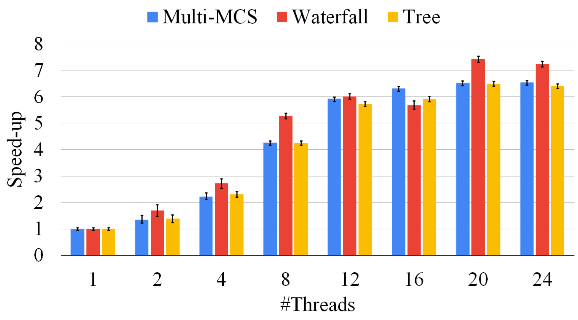
Compared to the two waterfall strategies previously analyzed, the tree approach has the advantage of allowing separate computing units to work on different graph pairs. In the waterfall approach, due to the inherently unbalanced nature of the problem, doubling the number of threads does not always imply halving the solution time. On the contrary, solving graph pairs in parallel, as in the tree approach, reduces contention and provides better speed ups compared to the case in which the effort of all threads focuses on the same graph pair. In other words, instead of adding more computational power to a single pair of graphs as the waterfall approach, the tree strategy solves multiple graph pairs in parallel, improving the scalability of the method thanks to the presence of unrelated tasks. This also allows us to include a GPU (or multiple computers) in the computation without the necessity of introducing any sort of advanced synchronization. The disadvantage of the tree strategy is that we only consider one solution for each MCS problem, discarding a larger portion of the search space and potentially reducing the size of the final result. Furthermore, although the approach allows for better scaling, it does not guarantee that, given the same number of threads, it will outperform the previous method. We observed multiple times that the previous approach was both faster and produced a larger common subgraph. This behavior is caused by the fact that we wait for all graph pairs to be solved before generating the pairs from their solutions. This choice means that the time to be spent on a group of graphs is bound by the time spent to solve the pair of graphs that takes the longest. To mitigate this problem, we introduced a unified thread pool that allowed for any single threads to move from one pair of graphs to another; while this feature reduced the independence of the different MCSs, it allowed for a quicker run time on a single machine.

4.4. A Mixed CPU-GPU Tree Approach

To improve the performances of our algorithms, we ran some experiments adding a GPU to the standard power computation of the CPU. We explored two main approaches:

• Using the GPU as an additional computational unit in the thread pool of the waterfall approach.
• Using the GPU as a separate computing unit to offload some of the graph pairs in the tree method.

The first approach consists in dedicating a portion of the CPU computation power to produce partial problems to transfer to the GPU. The GPU, having at its disposal thousands of threads, can then solve each problem independently. While the GPU is busy with this work, the CPU can work on other instances following the original McSplit logic. Unfortunately, this approach does not bring relevant advantages to the overall computation time; on the fastest run, it usually marginally slows down the process. More specifically, this algorithm only shows significant speed ups when the workload is evenly distributed between threads, but cannot improve under a significant workload unbalance. Unfortunately, a medium-to-strong unbalanced workloads is present in the vast majority of the cases.

The second approach shows the ability of splitting the process among different computational units along the tree approach. Instead of letting the CPU solve all of the graph pairs, we move one pair to the GPU to reduce the workload on the CPU and improve the overall performance. However, the setup (and data loading phase) required to run the GPU take quite a long time, and as such, the process is unfit for the solution of small graph pairs. Nonetheless, this approach shows significant improvements in the more challenging instances, decreasing the solution time up to a factor of two.

The GPU version mentioned in this section is an extension of the one discussed by Quer et al. [17]. The original version received two main extensions to improve its efficiency:

• Since the original version had a tendency to take a significant amount of time to resolve stand-alone instances of graph pairs, we created a buffer of problems to pass to the GPU. In this way, the GPU kernel can process several high-complex sub-problems before needing new data or instructions from the CPU.
• To increase the collaboration among GPU threads, we use the global memory to share some information, such as the size of the MCS found up to that moment. This value tends to change with a quite low frequency. It can therefore be easily maintained and updated in the device cache.

5. Sorting Heuristics

This section is divided into two parts. Section 5.1 describes a heuristic, suited for any number of graphs, to sort multi-domains, domains, and vertices. Section 5.2 reports some techniques to sort graphs when multiple graphs are involved.

5.1. Domains Sorting Heuristics

In this section, we propose a sorting heuristic taking into considerations bidomains (or multi-domains), domains, and vertices (please, see Section 3.1 for the definition of these objects). Our heuristic can be applied to all our approaches and implies only minor modification to the original procedure written by McCreesh et al. [28]. However, for the sake of simplicity, we mainly focus on graph pairs and describe how to extend the heuristics to multiple graphs.

To quickly prune the solution space, function selectFirstNode (please, see Algorithm 1) selects a new vertex pair in two steps. It first chooses the bidomain in which the largest domain includes the smallest number of nodes. Then, it selects the vertex with the smaller degree in the first graph and tries to pair it with each node in the second graph belonging to the same bidomain. Since the target is to prune the search as soon as possible, discarding a node from the solution reduces the bound only if the node belongs to the smallest domain of the bidomain. Consequently, once we have selected a bidomain, we rearrange its domains to proceed on the graph with the smallest domain. This heuristic can be trivially extended to multiple graphs, as its reasoning remains unchanged. Instead of selecting a bidomain, the algorithm chooses a multi-domain from which to select subsequent vertices. As in the example with two graphs, we still want to rearrange the domains in such a way that the first one to be solved is the smallest of the group since it will be the one to have the more significant impact on the bound computation. The more prominent the difference between the sizes of the two domains, the more significant effect this variation has. We perform several experiments using this strategy with different heuristics to select the bidomain. We experimented with both the original strategy and some variations; thus, we select the bidomain with the largest domain, the one with the smallest domain, the one with the minimum product between domain sizes, and the minimum sum of domain sizes. In almost all the tests carried out, the original strategy proved to be the most effective. Therefore, all the tests in the following sections are carried out using it.

Table 3 shows how selecting the right domain from a bidomain can change the bound computation. Table 3a illustrates the initial bidomain configuration for graphs $G_1$ and $G_2$. Table 3b shows the case in which we select the domain of $G_1$. We try to pair all vertices of $G_1$ with all vertices of $G_2$. In this way, we remove one vertex from the first domain every two recursive calls, one for each node contained in the second domain. Consequently, the bound only changes after nine recursive calls since the smallest of the two domains still includes two nodes. In Table 3c, we select the domain on the second graph, which is the smallest of the two. At first sight, this is a worse sequence of tests since it takes five steps instead of two to remove a vertex from the domain. Nonetheless, as soon as the vertex a is discarded, at step six, the smallest of the two domains counts only one vertex; therefore, the bound is decreased by one after six recursive calls.

Table 3. An example to illustrate the pruning effect of a smart bidomain sorting heuristic.

a  Bidomain

b  Matchings without sorting domains

c  Matchings on sorted domains

${\mathit{G}}_1$

${\mathit{G}}_2$

Step

Nodes

Match

Bound

Step

Nodes

Match

Bound

$\mathit{v}$

$\mathit{L}$

$\mathit{v}$

$\mathit{L}$

1

$G_1$ = {1, 2, 3, 4, 5} $G_2$ = {a, b}

1 - a

2

1

$G_2$ = {a, b} $G_1$ = {1, 2, 3, 4, 5}

a - 1

2

1

x

a

x

2

$G_1$ = {1, 2, 3, 4, 5} $G_2$ = {a, b}

1 - b

2

2

$G_2$ = {a, b} $G_1$ = {1, 2, 3, 4, 5}

a - 2

2

2

x

b

x

3

$G_1$ = {2, 3, 4, 5} $G_2$ = {a, b}

2 - a

2

3

$G_2$ = {a, b} $G_1$ = {1, 2, 3, 4, 5}

a - 3

2

3

x

4

$G_1$ = {2, 3, 4, 5} $G_2$ = {a, b}

3 - b

2

4

$G_2$ = {a, b} $G_1$ = {1, 2, 3, 4, 5}

a - 4

2

4

x

5

$G_1$ = {3, 4, 5} $G_2$ = {a, b}

3 - a

2

5

$G_2$ = {a, b} $G_1$ = {1, 2, 3, 4, 5}

a - 5

2

5

x

6

$G_1$ = {3, 4, 5} $G_2$ = {a, b}

3 - b

2

6

$G_2$ = {b} $G_1$ = {1, 2, 3, 4, 5}

…

1

7

$G_1$ = {4, 5} $G_2$ = {a, b}

4 - a

2

8

$G_1$ = {4, 5} $G_2$ = {a, b}

4 - b

2

9

$G_1$ = {5} $G_2$ = {a, b}

…

1

Table 3. An example to illustrate the pruning effect of a smart bidomain sorting heuristic.

a  Bidomain

b  Matchings without sorting domains

c  Matchings on sorted domains

${\mathit{G}}_1$

${\mathit{G}}_2$

Step

Nodes

Match

Bound

Step

Nodes

Match

Bound

$\mathit{v}$

$\mathit{L}$

$\mathit{v}$

$\mathit{L}$

1

$G_1$ = {1, 2, 3, 4, 5} $G_2$ = {a, b}

1 - a

2

1

$G_2$ = {a, b} $G_1$ = {1, 2, 3, 4, 5}

a - 1

2

1

x

a

x

2

$G_1$ = {1, 2, 3, 4, 5} $G_2$ = {a, b}

1 - b

2

2

$G_2$ = {a, b} $G_1$ = {1, 2, 3, 4, 5}

a - 2

2

2

x

b

x

3

$G_1$ = {2, 3, 4, 5} $G_2$ = {a, b}

2 - a

2

3

$G_2$ = {a, b} $G_1$ = {1, 2, 3, 4, 5}

a - 3

2

3

x

4

$G_1$ = {2, 3, 4, 5} $G_2$ = {a, b}

3 - b

2

4

$G_2$ = {a, b} $G_1$ = {1, 2, 3, 4, 5}

a - 4

2

4

x

5

$G_1$ = {3, 4, 5} $G_2$ = {a, b}

3 - a

2

5

$G_2$ = {a, b} $G_1$ = {1, 2, 3, 4, 5}

a - 5

2

5

x

6

$G_1$ = {3, 4, 5} $G_2$ = {a, b}

3 - b

2

6

$G_2$ = {b} $G_1$ = {1, 2, 3, 4, 5}

…

1

7

$G_1$ = {4, 5} $G_2$ = {a, b}

4 - a

2

8

$G_1$ = {4, 5} $G_2$ = {a, b}

4 - b

2

9

$G_1$ = {5} $G_2$ = {a, b}

…

1

In general, our heuristic works at its best when the domains with the same label have a different size. As a consequence, it generates better results when applied to larger instances, where less homogeneous domain sizes could be found, and to graph sets where the graphs have different numbers of nodes.

5.2. Graph Sorting Heuristics

The efficiency of the sequential and the parallel approaches directly depends on the structure of the graphs. At the same time, the pruning effect is proportional to the ability of the procedure to find large common subgraphs quickly. As a consequence, the execution time of all strategies is strongly influenced by the order in which the graphs are considered. With graphs of different sizes, their relative order can significantly impact the solution time.

Given the set of graphs $\{G_1,G_2,\dots ,G_N\}$, we conducted experiments using various heuristics:

• We consider them in random order.
• We sort them based on the number of vertices in ascending and descending order.
• We sort them based on the number of vertices. Then, we select one graph at each extreme of the list, i.e., we start with the smallest graph, followed by the biggest, then by the second smallest, the second biggest, etc.

These sorting techniques perform differently on the different strategies (i.e., Multi-MCS, waterfall, multi-way waterfall, tree, etc.), and we analyze each of them in the following subsections.

5.2.1. Heuristics for the Exact Approaches

For the exact approaches (either the sequential or the parallel one) and pairs of graphs, it is sufficient to use the graph with the smallest number of nodes as the first element of the algorithm to see a substantial increase in performance. To handle more graphs, the number of possible permutations increases very rapidly. As for pairs of graphs, it is essential to ensure that the first graph is the one of minimum size, as this strategy alone may reduce the execution time to more than an order of magnitude. Changing the order of subsequent graphs has a minor effect until it becomes negligible after the first four to five graphs. Our first attempt was to sort graphs considering their size in ascending order. A closer analysis showed that this assumption was incorrect and that selecting one graph at each extreme of the list (i.e., starting with the smallest graph, followed by the biggest, then by the second smallest, the second biggest, etc.) delivers the best results. It is essential to notice that the graph order is important even when dealing with graphs of the same size, even if we were unable to find any heuristic able to produce consistently better results than a random sorting.

5.2.2. Heuristics for the Waterfall Approach

The waterfall approach is the methodology for which an optimal sorting can bring the most significant benefits regarding execution time and solution size. Unlike the exact approaches, with the waterfall strategy, there is no advantage in sorting the graphs in an oscillating order (minimum size, maximum, second minimum, etc.) and a simple sorting by increasing size is the best option. From our results, the earlier the most extensive graphs are used along the computation, the smaller the final solution. Consequently, considering the largest graphs before the others not only slows down the process but also degrades the quality of the final solution. We theorized that this behavior is due to the fact that the largest graphs are also the ones that have the highest probability of preserving the size of the solution returned by the previous steps. Therefore, using one of these graphs in the first steps of the solution is equivalent to a rapid loss of information that will, on average, lead to a deterioration of the final solution. At the same time, finding a solution between two small graphs (or between a small and a large graph) takes exponentially less time than considering two large graphs; thus, following an increasing ordering combines both of these advantages.

5.2.3. Heuristics for the Tree Approach

Since the tree approach is based on finding solutions for pairs of graphs, many of the considerations reported in the previous subsection can be repeated for this algorithm. Nonetheless, some key considerations must be made concerning the order in which the solutions must be considered. Since all graphs, including the largest ones, must be examined at each step, we cannot keep any graph aside to preserve the solution quality. Therefore, we tested two possibilities, pairing:

• The smallest graph with the largest graph, the second smallest with the second largest, etc.
• The smallest graph with the second smallest, the third smallest with the fourth smallest, etc.

Although the second approach generates larger solutions on average, improvements are marginal. However, at the same time, it is also drastically worse in terms of execution time as it considers the largest graphs together. As a consequence, we test the tree approach with the first order, favoring a much shorter solution time over the occasional improvement in the size of the reported solution.

6. Experimental Results

In this section, we first present our experimental setting in terms of hardware, software, and benchmarks used (Section 6.1). Then, we evaluate our sorting (bidomain and graph-oriented) heuristics (Section 6.2). Finally, we present our results on the Multi-MCS and Multi-quasi-MCS problem (Section 6.3).

6.1. Setting

We ran all tests on a workstation equipped with a CPU Intel Core i9-10900KF (with 10 cores and 20 threads), 64 GB DDR4 of RAM, and a GPU NVidia GeForce RTX 3070. We wrote all our code in C++ (compiled with gcc 9.4.0), and we used CUDA (version 11.6) for the GPU implementation.

We tested our code using the ARG benchmark graphs generated by Foggia et al. [30] and De Santo et al. [31]. This database is composed of several classes of graphs, randomly generated according to six different strategies with various characteristics, such as size, density, topology, similarity, etc. The result is a huge data set [32] of 168 different types of graphs and a total of 166,000 different graphs. In our experimental setup, we only consider a subset of this data set, limited to about 500 graph sets, and we select it randomly from the original set.

In all experiments involving graph pairs, we adopt a timeout of 100 s. On sets of graphs of increasing size, we extend our timeout to 1000 s or 3600 s (i.e., one hour). As the scheduling (and context switching) of the operating system may vary the way in which threads are executed, we run each test ten times, and we present the average result and its standard deviation in each case.

In all tests, the memory used is always limited to 10 MBytes, posing no issue on modern hardware architectures. Since this value does not change significantly, not even in the multi-threaded versions, we will not further report considerations on the memory used by our applications.

All our functions (in the C and C++ languages), all benchmarks, experimental settings, and results are available on GitHub [33].

6.2. Sorting Results

In this section, we compare the sorting heuristic of Section 5.1 with the original strategy adopted by McSplit. Moreover, to evaluate an upper-bound for the speed up the heuristic can generate, we compare it with a version of McSplit adopting a reverse order, i.e., the one in which we select bidomains (or multi-domains) starting from the largest (not the smallest) number of nodes.

In Figure 9, we present experiments on 500 graph pairs in which the 2 graphs have the same size. We extract the graphs from the whole data set, sampling each class of graphs as uniformly as possible. Figure 9 reports two histograms. On the left-hand side, we compare the average solution time against the original algorithm and the one using the reverse order. On the right-hand side, we compare the number of vertex pairs considered by the same three heuristics. Both histograms are normalized with respect to the original time and the number of vertices considered, respectively. The left-hand plot shows that our heuristic outperforms the state-of-the-art approach by around 10% on average. On the contrary, by sorting the domains in reverse order, the figure shows a slowdown by about 20%. The right-hand plot shows that our heuristic also prunes the state space visited (i.e., it reduces the number of pairs checked) of about 15% when compared to the state-of-the-art approach and 25% when compared with the reverse order. In all cases, the standard deviation indicated on the top of each bar shows that data are clustered around the mean value. We found very similar results for sets of three, four, and five graphs; however, we do not report the plots for the sake of space. The reason to explain why our sorting heuristic prunes the solution space more efficiently lies in the bound computation strategy. McSplit is a “fail-first” algorithm that checks the vertex pairs that most likely will quickly prune the solution space before the others. As shown in Section 2, the bound is computed as the sum of the dimensions of the smallest domain belonging to each bidomain. After attempting every possible match with a certain node, the original algorithm tries to proceed without selecting it as part of the solution, thus, reducing the size of the respective domain. However, as all nodes of the first of the two graphs are considered, only the domains of the first graph decrease in size as the execution proceeds. Our heuristic ensures that the first of the domains is always the smallest and, consequently, the one that affects the bound calculation more effectively. Thus, our strategy improves the bound computation and discards superfluous portions of the search space more efficiently.

Although Figure 9 focuses on graphs of the same size, our sorting heuristic may have a larger impact on graph pairs of different sizes. For that reason, Figure 10 presents the same set of experiments of Figure 9 on 500 graph pairs randomly selected, i.e., without ensuring that the graphs have the same size. In this situation, the average execution time is reduced by more than 50%, and the state space is pruned by more than 60%. The reverse sorting slows down the average execution time by almost 50%. Moreover, the heuristic works better when the difference between the graph size is larger and the graphs are larger. As in the previous experiment, notice that the standard deviation is close to zero in all cases, proving that data are clustered around the mean value and that multi-threading returns consistent results. As for Figure 9, we found very similar results for sets of three, four, and five graphs; however, we do not report the plots for the sake of space. These results prove that our heuristic is quite general and beneficial in all conditions.

6.3. Results on the Multi-MCS Problem

In this section, we first analyze how parallelization can improve the performance of our algorithms when we use an increasing number of threads (Figure 11). Then, we show how the three main approaches scale on graph sets formed by more than two graphs (Figure 12, Figure 13 and Figure 14). Finally, considering the waterfall approach the most meritorious, we show how varying the number of intermediate solutions retained affects both the execution time and the quality of the final solution (Figure 15 and Figure 16).

Figure 11 shows the speed ups we can obtain by increasing the parallelism level of our procedures. Similarly to the previous section, we run our experiments on 500 graph pairs of different sizes. For each pair, we present average results over ten runs. Figure 11 shows that all the approaches scale similarly. However, we notice that even if they converge to similar results, solving harder graphs brings a larger degree of variability, since a single thread could be stuck on an extremely hard and lengthy branch of the exploration, defeating the advantages of having a large number of threads. Notice that the parallel implementations are far from their ideal behavior, and the computation time does not linearly scale with the number of threads. We can obtain an average speed up slightly higher than 6 with 24 threads. This behavior is mainly due to the fact that the MCS problem is innately unbalanced. The original McSplit algorithm also suffers from the same problem when dealing with graph pairs. As a final consideration, we point out that even if the tree approaches should scale better than the other methods, Figure 11 seems to show that this is not true. This behavior is due to the fact that we divide multiple problems over the cores of a single workstation, whereas we could distribute the same workload over a significantly larger number of machines. Moreover, the same methodology would be inapplicable to the other approaches since they run a single MCS at a time. In all the following experiments, we adopt 12 threads, as this looks like the configuration with the better trade off between the number of threads and performances.

Figure 12 compares the same three strategies, i.e., the Multi-MCS strategy (of Section 3.2) and the Multi-quasi-MCS strategies of waterfall and tree (of Section 4.1 and Section 4.3, respectively), reporting the number of instances solved. We focus on 390 triples of graphs and, as in the previous sections, we run each experiment ten times. The y-axis indicates the number of instances solved as a function of the time passed. Small fluctuations on this axis are due to the representation of the standard deviation, that, as in the previous experiments, is always very low and indicates that all runs are close to the mean one. For these tests, we set the time limit to 100 s, since most of the instances required a limited solution time. As far as the elapsed time is concerned, the graphic clearly shows that the two Multi-quasi-MCS approaches are orders of magnitude faster than the Multi-MCS algorithm. As depicted in Figure 12, the performance gap actually increases with the larger graph triplets, as already assumed in Section 4.1 and Section 4.3, where we discussed the complexity of those approaches. As mentioned in Section 4.3, the tree approach is faster than the waterfall procedure. However, the tree approach is also the one finding the smaller solutions. On 390 graph triplets, the tree approach returns results with approximately 0.37 fewer nodes than the waterfall procedure on average. Similarly, the waterfall approach returns results with approximately 0.24 fewer nodes than the exact Multi-MCS procedure on average. Since the exact MCS has an average size of 15.56 nodes, we can estimate that the waterfall approach can approximate the exact solution with 98.5% accuracy, while the tree approach can reach 96.3% accuracy.

Figure 13 extends the previous analysis to sets of six graphs. To show the flexibility of the tree approach, we test it by adding a GPU as a secondary computing unit, offloading a portion of the work from the CPU. As already explained in Section 4.4, our GPU algorithm is not yet ready to substitute the CPU implementation on all instances. For example, the GPU exhibits a moderate initial latency and overhead, especially for smaller instances, as well as a significant increase in the amount of RAM used. These characteristics are also shown by the higher standard deviation of the data obtained and represented by the larger fluctuations of the plot on the y-axis. The communication protocol between the CPU and the GPU causes some latency that can vary significantly between runs. Nonetheless, after the initial delay, the coordinated effort of more computational units, thanks to its optimized workload distribution, managed to catch up to the CPU-only version. Moreover, we managed to run all tests in less than 500 MBytes. Figure 13 clearly shows that an exact approach is an extremely challenging computational problem in the more problematic instances. As far as the accuracy of our approaches is concerned, if we compare the size of the solution for those cases in which all procedures managed to finish before the timeout of 1000 s, we see that the waterfall approach reaches a 98.5% accuracy, whereas the tree approach plummeted to only 65.4%.

To further deepen our analysis, Figure 14 extends Figure 12 and Figure 13, considering an increasing number of graphs, varying from two to twelve. The x-axis reports the number of graphs. The y-axis indicates the average solution time of each set of graphs of the exact, the waterfall, and the tree approach. We compute the mean value over 50 sets of graphs, and we normalize all data with respect to the resolution time for sets of two graphs. For the y-axis, we also use a logarithmic scale and we extend the timeout to 3600 s (i.e., one hour). The graph shows that the exact approach is definitely unable to manage an increasing number of graphs as, even adopting the pruning of the original McSplit procedure, it must manage huge search spaces. Thus, the exact approach is ${10}^8$ times slower than the approximate approaches for sets with more than eight graphs, and it essentially run out of time. On the contrary, the approximate approaches hardly require a larger average time as the number of graphs increases. This behavior is motivated by the fact that intermediate solutions are smaller than the original graphs and, consequently, extremely fast to compute. As a consequence, our strategies preemptively discard a large portion of the search space; thus, even if we do not wish to ignore the importance of an exact approach, we believe that the only viable option to manage large set of graphs is to exploit approximate algorithms.

As described in Section 4.2, one of the relevant features of the waterfall approach is that it allows us to store multiple intermediate solutions to improve the size of the result. Figure 15 shows how the number of intermediate solutions taken into consideration improves the size of the final result. However, we proved that the higher the number of intermediate solutions considered, the lower the improvement in the final solution. In conclusion, there is no significant benefit to maintaining a huge number of intermediate solutions.

Although the buffer size has a significant impact on the accuracy of the approach, it also has a limited effect on the computation time. Figure 16 plots the number of solved instances as a function of the elapsed time for several different buffer sizes (ranging from 1 to 100). These plots allow us to find the best-desired trade off between accuracy and computation efficiency. Intermediate solutions are saved as adjacency matrices, and only vectors containing partial and temporary information are needed to trace the nodes of the graphs from which the current one was generated. This compact representation hardly significantly affects the limited memory usage. As a consequence, in all cases, the quantity of memory used is limited to 25 MBytes.

7. Conclusions and Future Works

The MCS problem is an intrinsically unbalanced task. This feature is more pronounced with more complex graphs where the exhaustive exploration of a branch can require exceptionally long running times. Although incredibly memory efficient, our proposed exact approaches struggle to solve even minimal graphs when large enough numbers exist. As a consequence, we discuss a set of heuristics to trade off accuracy and computation time. Our waterfall and tree approaches have comparable running times, but, on average, the first finds more extensive final solutions. The tree approach can have some edge over the other methods in more powerful machines or multiple devices. We use a previous GPU implementation working on pairs of graphs to increase parallelization.

Among the future works, both the exact and the waterfall approaches can be further improved by developing the existing GPU implementation to autonomously work on sets of N graphs. In this case, the intrinsic disadvantages of the GPU (i.e., its initial latency and workload unbalance), can be leveraged by the effort on larger tasks. We would also like to work on an implementation able to solve the unbalanced nature of the current algorithm, thus significantly boosting its efficiency. This approach would also allow us to produce, later on, a version of the GPU algorithm that can fully exploit all the cores in the device, reducing its idle time. Moreover, as with an increasing number of graphs, the sorting strategies become more valuable, we would like to study alternative ordering heuristics. In this area, we mention the possibility of investigating the use of different graph properties with their related distributions and similar metrics used in other domains, such as the one of multiple sequence alignment [34].

References

1. Conte, D.; Foggia, P.; Sansone, C.; Vento, M. Thirty Years of Graph Matching in Pattern Recognition. Int. J. Pattern Recognit. Artif. Intell. 2004, 18, 265–298. [Google Scholar] [CrossRef]
2. Milgram, S. The Small World Problem. Psychol. Today 1967, 2, 60–67. [Google Scholar]
3. Watts, D.J. Networks, Dynamics, and the Small-world Phenomenon. Am. J. Sociol. 1999, 105, 493–527. [Google Scholar] [CrossRef] [Green Version]
4. Kleinberg, J.M. Authoritative Sources in a Hyperlinked Environment. J. ACM (JACM) 1999, 46, 604–632. [Google Scholar] [CrossRef] [Green Version]
5. Heymans, M.; Singh, A.K. Deriving Phylogenetic Trees from the Similarity Analysis of Metabolic Pathways. Bioinformatics 2003, 19, i138–i146. [Google Scholar] [CrossRef] [PubMed] [Green Version]
6. Dalke, A.; Hastings, J. FMCS: A Novel Algorithm for the Multiple MCS Problem. J. Cheminform. 2013, 5, O6. [Google Scholar] [CrossRef] [Green Version]
7. Park, Y.; Reeves, D. Deriving Common Malware Behavior through Graph Clustering. In Proceedings of the 6th ACM Symposium on Information, Computer and Communications Security (ASIACCS’11), Hong Kong, China, 22–24 March 2011; pp. 497–502. [Google Scholar] [CrossRef]
8. Bron, C.; Kerbosch, J. Finding All Cliques of an Undirected Graph (algorithm 457). Commun. ACM 1973, 16, 575–576. [Google Scholar] [CrossRef]
9. Barrow, H.G.; Burstall, R.M. Subgraph Isomorphism, Matching Relational Structures and Maximal Cliques. Inf. Process. Lett. 1976, 4, 83–84. [Google Scholar] [CrossRef]
10. Levi, G. A Note on the Derivation of Maximal Common Subgraphs of two Directed or Undirected Graphs. Calcolo 1973, 9, 341–352. [Google Scholar] [CrossRef]
11. Vismara, P.; Valery, B. Finding Maximum Common Connected Subgraphs Using Clique Detection or Constraint Satisfaction Algorithms. In Communications in Computer and Information Science; Springer: Berlin/Heidelberg, Germany, 2008; pp. 358–368. [Google Scholar] [CrossRef]
12. McCreesh, C.; Ndiaye, S.N.; Prosser, P.; Solnon, C. Clique and Constraint Models for Maximum Common (Connected) Subgraph Problems. In Principles and Practice of Constraint Programming, Proceedings of the 22nd International Conference, CP 2016, Toulouse, France, 5–9 September 2016; Lecture Notes in Computer Science; Springer: Cham, Switzerland, 2016; pp. 350–368. [Google Scholar] [CrossRef] [Green Version]
13. Bahiense, L.; Manić, G.; Piva, B.; de Souza, C.C. The Maximum Common Edge Subgraph Problem: A Polyhedral Investigation. Discret. Appl. Math. 2012, 160, 2523–2541. [Google Scholar] [CrossRef] [Green Version]
14. Bai, Y.; Xu, D.; Gu, K.; Wu, X.; Marinovic, A.; Ro, C.; Sun, Y.; Wang, W. Neural Maximum Common Subgraph Detection with Guided Subgraph Extraction. In Proceedings of the International Conference on Learning Representations (ICLR 2020), Addis Ababa, Ethiopia, 30 April 2020. [Google Scholar]
15. Bai, Y.; Xu, D.; Sun, Y.; Wang, W. GLSearch: Maximum Common Subgraph Detection via Learning to Search. In Proceedings of the Machine Learning Research, 38th International Conference on Machine Learning, Virtual Event, 18–24 July 2021; Meila, M., Zhang, T., Eds.; Volume 139, pp. 588–598. [Google Scholar]
16. Liu, Y.; Li, C.M.; Jiang, H.; He, K. A Learning Based Branch and Bound for Maximum Common Subgraph Related Problems. Proc. AAAI Conf. Artif. Intell. 2020, 34, 2392–2399. [Google Scholar] [CrossRef]
17. Quer, S.; Marcelli, A.; Squillero, G. The Maximum Common Subgraph Problem: A Parallel and Multi-Engine Approach. Computation 2020, 8, 48. [Google Scholar] [CrossRef]
18. Hariharan, R.; Janakiraman, A.; Nilakantan, R.; Singh, B.; Varghese, S.; Landrum, G.; Schuffenhauer, A. MultiMCS: A Fast Algorithm for the Maximum Common Substructure Problem on Multiple Molecules. J. Chem. Inf. Model. 2011, 51, 788–806. [Google Scholar] [CrossRef]
19. Cormen, T.H.; Leiserson, C.E.; Rivest, R.L.; Stein, C. Introduction to Algorithms, 4th ed.; The MIT Press: Cambridge, MA, USA, 2022. [Google Scholar]
20. McCreesh, C.; Prosser, P.; Trimble, J. A Partitioning Algorithm for Maximum Common Subgraph Problems. In Proceedings of the Twenty-Sixth International Joint Conference on Artificial Intelligence (IJCAI-17), Melbourne, Australia, 19–25 August 2017; pp. 712–719. [Google Scholar] [CrossRef] [Green Version]
21. McGregor, J.J. Backtrack Search Algorithms and the Maximal Common Subgraph Problem. Softw. Pract. Exp. 1982, 12, 23–34. [Google Scholar] [CrossRef]
22. Balas, E.; Yu, C. Finding a Maximum Clique in an Arbitrary Graph. SIAM J. Comput. 1986, 15, 1054–1068. [Google Scholar] [CrossRef]
23. Raymond, J.W.; Willett, P. Maximum Common Subgraph Isomorphism Algorithms for the Matching of Chemical Structures. J. Comput.-Aided Mol. Des. 2002, 16, 521–533. [Google Scholar] [CrossRef] [Green Version]
24. Ndiaye, S.M.; Solnon, C. CP Models for Maximum Common Subgraph Problems. In Principles and Practice of Constraint Programming (CP 2011); Springer: Berlin/Heidelberg, Germany, 2011; pp. 637–644. [Google Scholar] [CrossRef] [Green Version]
25. Piva, B.; de Souza, C.C. Polyhedral Study of the Maximum Common Induced Subgraph Problem. Ann. Oper. Res. 2012, 199, 77–102. [Google Scholar] [CrossRef] [Green Version]
26. Englert, P.; Kovács, P. Efficient Heuristics for Maximum Common Substructure Search. J. Chem. Inf. Model. 2015, 55, 941–955. [Google Scholar] [CrossRef]
27. Hoffmann, R.; McCreesh, C.; Reilly, C. Between Subgraph Isomorphism and Maximum Common Subgraph. In Proceedings of the Thirty-First AAAI Conference on Artificial Intelligence, San Francisco, CA, USA, 4–9 February 2017; pp. 3907–3914. [Google Scholar]
28. McCreesh, C. Solving Hard Subgraph Problems in Parallel. Ph.D. Thesis, University of Glasgow, Glasgow, UK, 2017. [Google Scholar]
29. Simon, J.; Larsen, J.B. CytoMCS: A Multiple Maximum Common Subgraph Detection Tool for Cytoscape. J. Integr. Bioinform. 2017, 14, 20170014. [Google Scholar] [CrossRef] [Green Version]
30. Foggia, P.; Sansone, C.; Vento, M. A Database of Graphs for Isomorphism and Sub-Graph Isomorphism Benchmarking. In Proceedings of the 3rd IAPR TC-15 International Workshop on Graph-Based Representations, Ischia, Italy, 23–25 May 2001; pp. 176–187. [Google Scholar]
31. De Santo, M.; Foggia, P.; Sansone, C.; Vento, M. A Large Database of Graphs and its Use for Benchmarking Graph Isomorphism Algorithms. Pattern Recogn. Lett. 2003, 24, 1067–1079. [Google Scholar] [CrossRef]
32. Available online: https://mivia.unisa.it/datasets/graph-database/arg-database/ (accessed on 23 March 2023).
33. Available online: https://github.com/stefanoquer/Multi-Maximum-Common-Subgraph (accessed on 23 March 2023).
34. Feng, D.; Doolittle, R. Progressive Sequence Alignment as a Prerequisitetto Correct Phylogenetic Trees. J. Mol. Evol. 1987, 25, 351–360. [Google Scholar] [CrossRef] [PubMed]
Figure 1. Given the graphs G 1 and G 2 represented in (a,b), (c) reports two different admissible MCSs. Labels are shown only to help identify the vertices.
Computation 11 00069 g001
Figure 2. Two undirected and unlabeled graphs G 1 , G 2 , and one possible common subgraph computed by McSplit. Node labels, i.e., { 1 , 2 , 3 , 4 } and { a , b , c , d } , are reported to uniquely identify all vertices.
Computation 11 00069 g002
Figure 3. Computing the MCS of N graphs { G 1 , G 2 , , G N } using a single branch-and-bound recursive function Multi-MCS ( G 1 , G 2 , , G N ).
Computation 11 00069 g003
Figure 4. Three undirected and unlabeled graphs, G 1 , G 2 , G 3 , and one possible common subgraph computed by McSplit. Node labels, i.e., { 1 , 2 , 3 , 4 , 5 } , { a , b , c , d , e , f } , and { A , B , C , D } are reported to uniquely identify all vertices.
Computation 11 00069 g004
Figure 5. The waterfall approach: computing Multi-quasi-MCS ( { G 1 , G 2 , , G N } ) as M C S ( , M C S ( M C S ( G 1 , G 2 ) , G 3 ) , , G N ) .
Computation 11 00069 g005
Figure 6. An example of three graphs { G 1 , G 2 , G 3 } for which the Multi-quasi-MCS waterfall approach finds an empty solution even if Multi-MCS ( { G 1 , G 2 , G 3 } ) has two nodes.
Computation 11 00069 g006
Figure 7. The improved waterfall approach: Each call to the MCS function computes multiple intermediate solutions. For each solution, we run a new sequence of MCS problems. A threshold heuristically limits the expansion tree.
Computation 11 00069 g007
Figure 8. The parallelizable tree approach: we compute Multi-quasi-MCS ( { G 1 , G 2 , , G N } ) as M C S ( M C S ( M C S ( G 1 , G 2 ) , M C S ( G 3 , G 4 ) ) , ) .
Computation 11 00069 g008
Figure 9. Our sorting heuristic against the state-of-the-art order and the reverse one on graph pairs of the same size. We report the mean resolution time (on the left-hand side) and the average number of vertex pairs checked (on the right-hand side) normalized with respect to the original method. The standard deviation of the ten runs is reported on top of each bar.
Computation 11 00069 g009
Figure 10. Our sorting heuristic against the state-of-the-art order and the reverse one on graph pairs of random size. We report the mean resolution time (on the left-hand side) and the average number of vertex pairs checked (on the right-hand side) normalized with respect to the original method. The standard deviation of the ten runs is reported on top of each bar.
Computation 11 00069 g010
Figure 11. Speed up of our algorithms using an increasing number of threads, varying from 1 (purely sequential) to 24. The plot compares the Multi-MCS strategy of Section 3.2, with the Multi-quasi-MCS strategies of Section 4.1, the waterfall strategy, and Section 4.3, the tree approach. We report average resolution times over 10 runs. The standard deviation of the ten runs is reported on top of each bar.
Computation 11 00069 g011
Figure 12. A comparison among the Multi-MCS, the waterfall, and the tree approaches. The plot reports the number of sets composed of three graphs solved as a function of the elapsed time. The fluctuations on the y-axis are due to the representation of the standard deviation over ten runs. The time limit is fixed at 100 s.
Computation 11 00069 g012
Figure 13. A comparison among the Multi-MCS, the waterfall, and the tree approaches. The plot reports the number of sets composed of six graphs solved as a function of the elapsed time. The fluctuations on the y-axis are due to the representation of the standard deviation over ten runs. The time limit is fixed at 1000 s.
Computation 11 00069 g013
Figure 14. A comparison among the Multi-MCS, the waterfall, and the tree approaches on sets of graphs with an increasing number of graphs, varying from two to twelve. The plot reports the average solution time over 50 sets of graphs. The resolution time is normalized with respect to the solution time of pair of graphs. The y-axis adopts a logarithmic scale.
Computation 11 00069 g014
Figure 15. The tree approach: Quality loss (on the y-axis) as a function of the number of intermediate solutions considered (on the x-axis), varying from 1 to 100.
Computation 11 00069 g015
Figure 16. The tree approach: Computation efficiency, i.e., normalized time taken to solve a given set of experiments as a function of the number of intermediate solutions stored (varying from 1 to 100).
Computation 11 00069 g016
Disclaimer/Publisher’s Note: The statements, opinions and data contained in all publications are solely those of the individual author(s) and contributor(s) and not of MDPI and/or the editor(s). MDPI and/or the editor(s) disclaim responsibility for any injury to people or property resulting from any ideas, methods, instructions or products referred to in the content.