Article

Fault-Tolerant Anomaly Detection Method in Wireless Sensor Networks

1
College of Engineering, Huaqiao University, Quanzhou 362000, China
2
Fujian Provincial Academic Engineering Research Centre in Industrial Intellectual Techniques and Systems, Quanzhou 362000, China
*
Authors to whom correspondence should be addressed.
Information 2018, 9(9), 236; https://doi.org/10.3390/info9090236
Submission received: 27 August 2018 / Accepted: 12 September 2018 / Published: 18 September 2018
(This article belongs to the Section Information and Communications Technology)

Abstract

:
A key issue in wireless sensor network applications is how to accurately detect anomalies in an unstable environment and determine whether an event has occurred. This instability includes the harsh environment, node energy insufficiency, hardware and software breakdown, etc. In this paper, a fault-tolerant anomaly detection method (FTAD) is proposed based on the spatial-temporal correlation of sensor networks. This method divides the sensor network into a fault neighborhood, event and fault mixed neighborhood, event boundary neighborhood and other regions for anomaly detection, respectively, to achieve fault tolerance. The results of experiment show that under the condition that 45% of sensor nodes are failing, the hit rate of event detection remains at about 97% and the false negative rate of events is above 92%.

1. Introduction

In recent years, wireless sensor networks (WSN) have been widely used in defense, military, healthcare, environmental monitoring, manufacturing, and many other fields [1,2]. They consist of a large number of nodes distributed in a geographical area, and are usually limited by the energy, storage capacity, computing power, and communication bandwidth. Wireless sensor networks mainly run in harsh, unattended environments where unreliable and dynamic changes often occur. Erroneous information generates a strong side effect on the subsequent control chain, leading to wrong decisions and inappropriate control actions. This paper presents a solution focused on anomaly detection, which include event and fault detection.
In event detection applications, nodes are responsible for determining whether specific events of interest occur within their sensing ranges. Theoretically, all sensor nodes in the event area should report the sensed information to the base station or sink node. In fact, due to environmental interference or hardware failure, sensor readings may be unreliable and may produce some erroneous sensor readings. Sensors may cause false alarms or missing reports, which will reduce the detection quality. One way to improve the event detection capability is to use fault-tolerant event detection schemes.
Many challenges exist to detect events efficiently. Firstly, it is challenging to develop a scheme for reliably detecting the interesting event under the circumstance of faulty nodes due to the fact that the node’s reading is unreliable. Secondly, the quality of event detection degrades rapidly, which motivates us to optimize the fault-tolerant event detection scheme [3].
How to reliably detect an event of interest in an unstable environment is one of the key problems in anomaly detection. Based on this, we propose a fault-tolerant anomaly detection method (FTAD) based on spatial-temporal correlation. The algorithm consists of two parts: the temporal correlation is used to obtain the probability of event and fault through the time-series data of sensor nodes, then we determine the state of sensor nodes. While according to the neighborhood definition, the sensor network is divided into the fault neighborhood, event and fault mixed neighborhoods, event boundary neighborhoods, and other areas, we use the minimum Bayesian risk decision method to distinguish the event nodes and faulty node. Fault tolerance is realized by abnormity detection to different neighborhoods, and experimental results and analysis show that the method can detect events well even under high fault rates.
The contributions of this paper are summarized as follows:
(i)
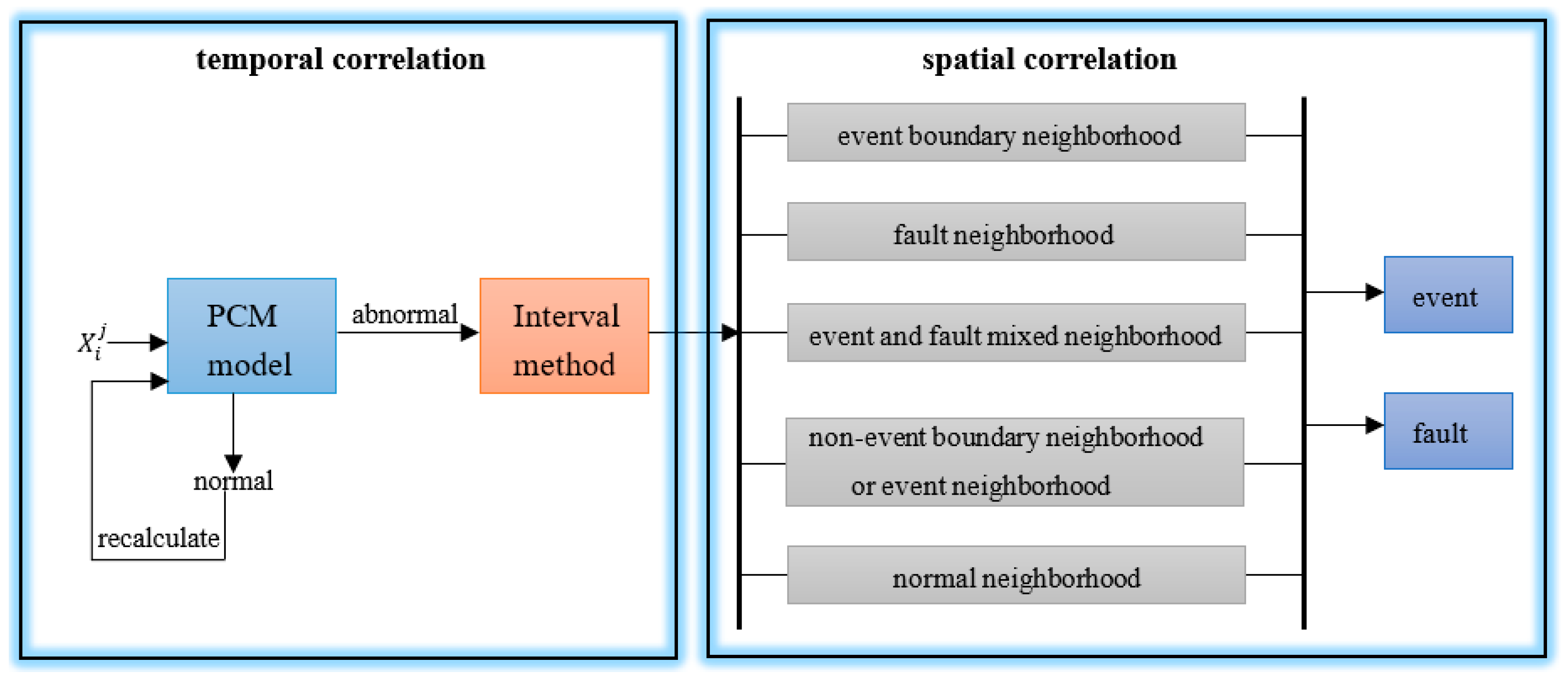
In temporal correlation of sensor network, we propose the PCM and interval methods;
(ii)
In spatial correlation we divide the sensor network into fault neighborhood, event and fault mixed neighborhood, event boundary neighborhood, and other regions for anomaly detection, respectively, to achieve fault tolerance.
(iii)
We conduct extensive simulations to evaluate the performance of the proposed algorithms. The results demonstrate the effectiveness of the proposed algorithms.
The second section introduces the related work and research results. The third section introduces the symbol definitions and network model used in this paper. The fourth section introduces the detection method of fault-tolerance of wireless sensor networks. The fifth section offers the results and analysis of the experiment. The final section concludes the paper.

2. Related Work

Anomaly detection algorithms can be categorized into five categories: statistical-based, nearest neighbor-based, classification-based, clustering-based, and spectral decomposition-based.
Statistical-based as the earliest anomaly detection method, is essentially based on the model. There are two types, parametric and non-parametric; the former one includes Gaussian and models based on regression, and the latter one includes histogram and kernel-based density function. Alippi et al. (2013) introduced a novel cognitive fault diagnosis system (FDS) for distributed sensor networks that takes advantage of spatial and temporal relationships among sensors. The proposed FDS relies on a suitable functional graph representation of the network and a two-layer hierarchical architecture designed to promptly detect and isolate faults. The lower processing layer exploits a novel change detection test (CDT) based on hidden Markov models (HMMs). Information provided by the CDT layer is then passed to the cognitive one, which, by exploiting the graph representation of the network, aggregates information to discriminate among faults, changes in the environment, and false positives induced by the model bias of the HMMs. From the experiment, even in highly noisy conditions, the proposed solution guarantees high detection accuracy and low detection delays [4]. Osanaiye et al. propose a step-wise approach using a statistical process control technique to detect DOS attacks. They deploy an exponentially-weighted moving average (EWMA) to detect anomalous changes in the intensity of a jamming attack event by using the packet inter-arrival feature of the received packets from the sensor nodes. Results obtained from a trace-driven simulation show that the proposed solution can efficiently and accurately detect jamming attacks in WSNs with little or no overhead [5]. Sousa et al. extend the model of the event detection scenario to distinguish between events and faults by using a flow chart and confidence interval. An event detection hit rate higher than 72% is obtained at 30% sensor faulty rate [6]. Cao combined with the spatial-temporal correlation of events to achieve fault tolerance by verifying the coincidence of time-series data with the statistical characteristics of stochastic processes [7]. Lo et al. presents a low-complexity distributive model-based diagnosis algorithm that identifies nonlinear sensor faults. An approximate solution to the LER problem is proposed for embedment in resource-constrained wireless sensors. By solving the LER problem, sensors corrupted by non-linearity faults can be isolated and identified [8]. Ntalampiras proposed a holistic modeling scheme for fault identification in distributed sensor networks [9]. The proposed scheme is based on modeling the relationship between two datastreams by means of a hidden Markov model (HMM) trained on the parameters of linear time-invariant dynamic systems, which estimate the specific relationship over consecutive time windows. Every system state, including the nominal one, is represented by an HMM and the novel data are categorized according to the model producing the highest likelihood. The system is able to understand whether the novel data belong to the fault dictionary, are fault-free, or represent a new fault type.
Nearest Neighbor Algorithm is also suitable for the detection of sensor network anomaly. Tang and Chow formulated a wireless sensor network (WSN) fault diagnosis problem as a pattern-classification problem and introduced a newly-developed algorithm, neighborhood hidden conditional random field (NHCRF), for determining hidden states between sensors [10]. The NHCRF model can improve the WSN fault diagnosis, because it has relaxed the independence assumption of the hidden Markov model. To enhance the robustness and antinoise ability of the NHCRF, the concept of nearest neighbors is used when estimating dependencies. Comparative results indicate that the method can deliver superior classification performance compared with other methods. Su et al. proposed a two-stage algorithm combining support vector machine and k-nearest neighbor (KNN), and procured a preferable effect by transforming time-series data into pattern anomaly detection [11]. Rashid et al. applied support vector machine, KNN, and a Gaussian mixture model to a multidimensional feature space to detect pipeline-specific events [12].
Existing methods for detecting outliers based on classification and clustering are mostly based on machine learning, such as support vector machine method, neural network, k-means algorithm, and adopting a Bayesian network. One-class support vector machine (OCSVM) is a widely used anomaly detection method. The OCSVM method is proposed by Miao et al., to obtain the decentralized implementation without transmitting the original data, uses a random approximate function to replace the kernel function [13]. Furthermore, to find an appropriate approximate dimension, and they add a sparse constraint into the decentralized cost function to obtain another one. Then they minimize these two cost functions by stochastic gradient descent and derive two distributed algorithms. Yang et al. presented a robust OCSVM [14]. In consideration that the contribution yielded by the outlying instances and the normal data is different, a robust one-class SVM which assigns an adapting weight for every object in the training dataset was proposed in [14]. Swain and Khilar presented a fault diagnosis protocol for wireless sensor networks (WSNs) based on a neural network approach [15]. A particle swarm optimization-based fuzzy multilayer perceptron is used in the fault detection and classification phase of the protocol. The proposed protocol considers the composite fault model such as hard permanent, soft permanent, intermittent, and transient fault. The result shows that the proposed protocol performs superior than the existing protocols. Zhao et al. formulate the WSN faulty node’s identification as a pattern classification problem [16]. The method uses semi-supervised method for faulty sensor nodes classification. To enhance the learning performance, it also introduces a label propagation mechanism which is based on local kernel density estimation. The basic concept of the method is to estimate the posterior probability of a scene that belongs to normal or different faulty modes. Experimental results show the proposed semi-supervised method is highly effective [16].
Outlier detection is based on spectral decomposition using principal component analysis (PCA) to identify normal behavior in wireless sensor networks. PCA is a data dimension reduction method to map high-dimensional data onto a relatively low-dimensional space before anomaly detection. Ghorbel et al. proposed an improved KPCA method based on the Mahalanobis kernel as a preprocessing step to extract relevant features for classification and to prevent abnormal events [17]. The literature [5,8,9,10,11,12,13,14,15,16,17] does not consider the fault-tolerant mechanism of event detection. Different fault-tolerant algorithms are used in [6,7], but the influence of faulty nodes on event detection is not considered; this approach proves to be ineffective in high-fault-rate sensor networks. Events will last for a period of time and cover a certain range when they occur, i.e., an event has a spatial-temporal correlation. Based on this, from the control chart and confidence interval method proposed in [6], obtaining the normal reading interval of the node, and combining the difference degree are applied to the temporal correlation part of this method. The Bayes theorem is used to calculate the probabilities of events or faults may occur in sensor nodes, then determine the state of sensor nodes. According to the definition of neighborhood, the sensor network is divided into a fault neighborhood, event and fault mixed neighborhoods, event boundary neighborhoods, and other areas to detect anomalies, respectively, and the event nodes and faulty nodes are distinguished by the minimum Bayesian risk decision.

3. Symbols and Network Model

In this paper, it is assumed that n sensor nodes are randomly scattered in a two-dimensional square area of d × d . Let S denotes the set of sensor nodes in this d × d region. The maximum communication radius of the sensor node is r , and the node S j within the communication radius is its neighbor node. The neighbor nodes form a neighbor region N . x j i as the reading of S j at time t i , which indicates the real measured value of the environment, such as temperature, humidity, noise, and so on. It is considered that the sensor node S j detects an event or a fault occurs when x j i exceeds the threshold R t h . We get the probability of events and faults through the time-series data of sensor nodes. If the probability of the occurrence of an event is greater than that of a fault, the sensor node S j is in the event state; if the probability of a fault is greater than that of an event, S j is in the fault state; otherwise S j in the normal state.
Defining the event based on readings of sensor nodes [18], when the event E occurs, the reading of sensor node in E is different from the outer E . The continuous area of the event is called the event area ε , and the remaining area is the normal area. The event area and normal area anomaly detection is defined as follows.
Definition 1:
Event boundary neighborhood B ( ε ) : sensor node S j is located in the event area and its neighborhood exists nodes both in the event state and in the normal state.
Since the faulty node will affect the accuracy of the detection in the event boundary neighborhood, it is necessary to exclude the influence of the faulty node, and the faulty node does not judge whether it is in the neighborhood of the event boundary.
Definition 2:
Non-event boundary neighborhood B ( ε ¬ ) : sensor node S j is located in the event area and not in the event boundary neighborhood B ( ε ) . That means its neighborhood may exist and that the nodes are in the event state, in the fault state, or in the normal state.
Definition 3:
Normal neighborhood N ( n ) : there are greater than N / 2 nodes in the normal state within the neighborhood. That is, most of nodes do not detect anomalies in the communication radius.
Definition 4:
Event neighborhood N ( ε ) : sensor node S j is located in the event area and the nodes are more than N / 2 in the event state. That is, most of the neighbor nodes may detect the event.
Definition 5:
Fault neighborhood N ( f ) : there more than N / 2 nodes in the fault state within the neighborhood. When the node is in N ( f ) , the method based on the assumption that the faulty node does not have spatial correlation [19,20,21] will determine the node as an event node, raise the false rate of the event and reduce the faulty node detection rate.
Definition 6:
Event and fault mixed neighborhood N ( ε f ) : The number of nodes in the neighborhood is greater than N / 2 , which are both in the event state and in the fault state. It is easy to misjudge the event node as the faulty node when the node in N ( ε f ) .
In this paper, the anomaly detection method based on the spatial-temporal correlation of sensor networks. Using the temporal correlation to obtain the probabilities of events or faults that may occur, to determine the state of sensor nodes. Then, we divided the sensor network into two regions: the event area and the normal area, and the area can be subdivided into different neighborhoods. In order to increase the detection rate and reduce the false alarm rate, each of them respectively detects the anomaly in different ways.
The symbols and terms used in this article are defined in Table 1.

4. Fault Tolerance Detection Method

This section will introduce, in detail, the fault-tolerant anomaly detection method. The algorithm consists of two parts: the temporal correlation (Algorithm 1) and the spatial correlation (Algorithm 2). In the temporal correlation part, the state of the node is preliminarily obtained, that is, the node may be in the event state, in the state of failure, or in the normal state. In the spatial correlation part, we divide the sensor network into the fault neighborhood, event and fault mixed neighborhood, event boundary neighborhood and other regions for anomaly detection and determine the final state of the node.

4.1. Temporal Correlation of Fault Tolerance Anomaly Detection Methods

This section is the temporal correlation of sensor network, firstly, it establishes a normal reference interval for each node of sensor network using time series data. Then, if the next sampling value is abnormal, it obtains the probabilities of an event or fault that may occur and determines the state of the node.

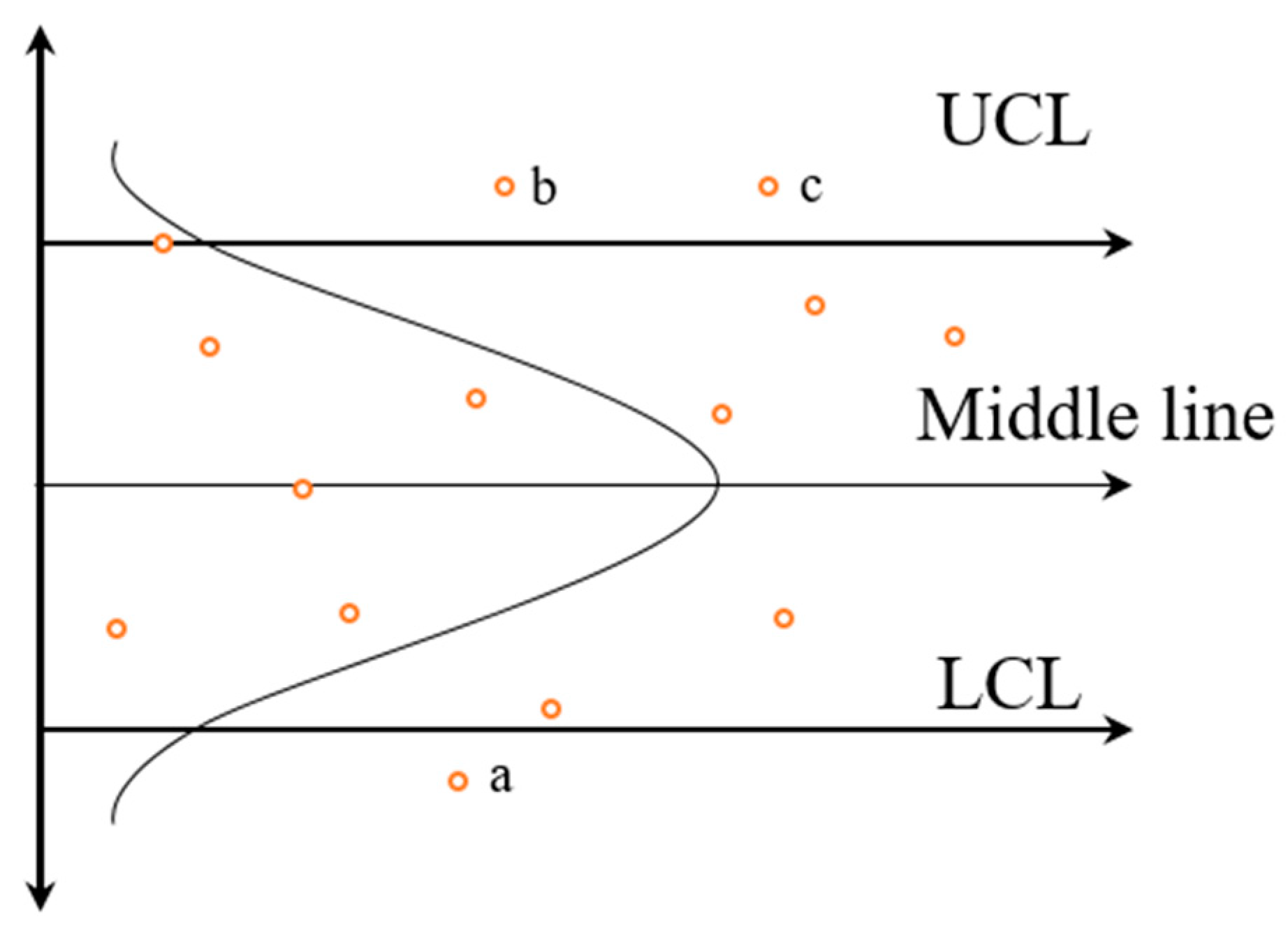
Pauta Criterion Method, PCM, and Interval Method

A. Pauta Criterion Method
A control chart method in the Theory of the Statistical Control Process [22] is an application of the Pauta Criterion. The first step to control a process statistically is to identify the process, the characteristics to be monitored, and to establish the most appropriate control chart. This control chart method is based on the average X ¯ of the control chart, but X ¯ is easily affected by the extreme value and the anomaly often appears to be the extreme value. Therefore, this paper uses the median m e d of the data set to create the control chart.
R = { x j 1 , x j 2 , , x j k } is the dataset of sensor node S j during T . The median and variance are expressed as follows:
m e d = { R [ k 2 ] + 1                 k   is   odd R [ k 2 ] + R [ k 2 ] + 1 2       k   is   even
σ m e d = 1 k i = 1 k ( x j i m e d ) 2
The Pauta Criterion has about 68%, 95%, and 99.7% of its values in the interval m e d ± c σ , with c = { 1 , 2 , 3 } respectively. In the interval formed by the m e d ± c σ , the measured value does not belong to this interval is 0.3%. As shown in Figure 1, the model consists of three lines: middle line (ML), which is the median of the sensor node dataset, and the upper and lower control lines (UCL and LCL). Let m e d be the median of the measurement middle and σ m e d be the standard deviation of the sensor node data set. These lines are calculated as follows:
M L = m e d
U C L = m e d + 3 σ m e d  
L C L = m e d 3 σ m e d
B. Interval Method
The detection method establishes a reference interval [ L C L , U C L ] by using the k data of the R = { x j 1 , x j 2 , , x j k } , which collected by the sensor node S j in the T period. The interval used to determine whether the sensor node detects an abnormality. If S j ’s reading x j i does not fall within this reference interval, an abnormality is detected, it may be an event or a fault occurring (see Algorithm 1).
We then calculate the probability of event and fault. S j is considered to be normal when it is reading x j i [ L C L , U C L ] , the interval difference is used to calculate the event probability p e , and the fault probability p f (see Algorithm 1).
γ = x j i U C L U C L - L C L  
where x j i is the reading of sensor node S j at time t ( i ) . γ represents the degree of difference between the reading and the interval at time t ( i ) . The larger γ the farther the sensor node readings are from the overall sample, the greater the probability for the outliers.
ξ = R t h ( t ) ( U C L - L C L )
R t h ( t ) = E n ( t ) + E e ( t ) 2
where R t h ( t ) is the threshold function for judging the event [7], E n ( t ) is the expected function of the correct reading of the sensor node in the normal area, and E e ( t ) is the expected function of the correct reading of the sensor node in the event area.
In summary, the establishment of a reference range of [ L C L , U C L ] by Pauta Criterion method. According to the interval to make judgments about whether the readings are abnormal or not. If x j i [ L C L , U C L ] , then calculate the probability of event p e and fault p f based on the interval method. If p e > p f , we think the node is in the event state, otherwise it is in the fault state.
Algorithm 1 describes the temporal correlation part of the algorithm. S donates the sensor node set of sensor network, let S j be the j th sensor node, R be the set collected by S j in T time period, x j i be the reading of sensor node S j at time t ( i ) , γ be the degree of difference between the reading and the interval at time t ( i ) , ξ is the degree of difference between the R t h ( t ) and the interval at time t ( i ) . p e and p f are the probability of an event and fault.
The statistical properties of the target variable, which the model is trying to predict, change over time in unforeseen ways. This causes problems because the predictions become less accurate as time passes. In order to deal with the problems of concept drift, in Algorithm 1 line 9 we recalculate the PCM model when x j i [ L C L , U C L ] .
Algorithm 1. Temporal correlation.
1://Calculate interval for each sensor node
2:    for each S j S do
3:           R Data sets collected during the T time period
4:              Calculate [ L C L , U C L ] using R
5:    end for
6://Detect if a sensor abnormal occurred.
7:    if x j i [ L C L , U C L ] then
8:              status = L N
9:              Recalculate [ L C L , U C L ]
10:    else
11:          calculate γ and ξ
12:             if γ > ξ then
13:                     p e increase
14:             end if
15:             if γ < ξ then
16:                     p f increase
17:             end if
18:    end if
19:    if p e > p f then
20:    status = L E
21:      else
22:             status = L F
23:    end if
24:    broadcasting status and { p e , p f } to all neighbors…
We analyze the asymptotic complexity of the algorithm in the worst case:
Line 4 and 9 calculates the reference interval in O ( k ) .
Lines 10–23 get the state of sensor nodes in O ( 8 ) .
This procedure is repeated for each sensor in the set S of sensors, yielding an overall complexity, in the worst case, of | S | × O ( k + 8 ) = O ( n ) .

4.2. Spatial Correlation of Fault Tolerance Anomaly Detection Methods

The sensor network has not only temporal correlation but also spatial correlation. The sensor nodes in the network can communicate with other sensor nodes in the form of a single-hop or multi-hop. In this paper, the sensor nodes communicate by using a single-hop, the maximum communication radius is r . The continuous area where the event occurs is denoted as the event area ε , and the other is called the normal area. The event area and the normal area are divided into different neighborhoods according to the given network model (Section 3), then anomaly detection is performed (see Algorithm 2)
Algorithm 2. Spatial correlation.
1:  receiving statuses and { p e , p f } from neighbors…
2:  if status = L N then
3:               continue
4:  else
5:         if S j in B ( ε ) then
6:                  S j final status equal last status
7:         end if
8:         if S j in N ( f ) then
9:                   if S j status is same most of neighbors then
10:                        S j final status is fault
11:                  else
12:                       S j final status is event
13:                  end if
14:         if S j in N ( ε f ) then
15:                      Compare f and e
16:         end if
17:         if S j in B ( ε ¬ ) or in N ( ε ) then
18:                  if S j status is same most of neighbors then
19:                          S j final status is event
20:                  else
21:                          S j final status is fault
22:                  end if
23:         if S j in N ( n ) then
24:                  if S j status is most same of neighbors then
25:                          S j final status is normal
26:                  else
27:                          S j final status is fault
28:                  end if
29:  end if
When the sensor node S j is located in the event boundary neighborhood B ( ε ) , in the fault neighborhood N ( f ) , or event and fault mixed neighborhood N ( ε f ) , this usually leads to erroneous or false judgments. Causes of that are analyzed as follows:
The event boundary neighborhood B ( ε ) is the boundary between the event area and the normal area. The sensor nodes in B ( ε ) contains both the normal node that detected the event and did not detect the event. It is easy to misjudge the event node as the faulty node when the numbers of nodes are detected as events less than N / 2 . There are two methods to determine whether a node is in the event boundary neighborhood or not:
Most of the principles: A node is identified at the event boundary only if this result is the main result within its neighborhood. According to statistics, this rule may lead to correcting errors even if the sensor failure rate is less than 50%. This rule was proved to be the best when using the Bayesian method [23].
Consistency principle: There is a deviation in the measured value of the faulty node. Assume that if a node does not obey most of the principles, its result will be ignored by its neighbors. At this time, consistency rules are used to enforce the consistency rules [24].
Using the principle of consistency, a node is considered to be in the event boundary neighborhood only when satisfying Equation (9):
m > n π a 2 d 2 ( 1 p )  
where n and d are the number of sensors and length of the sensor network, p is the failure rate of the sensor network, is a rounding down function, and m is the number of neighboring nodes. a is an acceptable event boundary width ( a < r ), specified by the user. If the number of neighbor nodes (both in the normal state and in the event state) satisfy Equation (9), then S j B ( ε ) .
If the sensor node S j is located in the fault neighborhood N ( f ) or in the event and fault mixed neighborhood N ( ε f ) , the faulty node will be misjudged to be an event node based on the method of faulty node isolation. When the sensor node S j is located in the fault neighborhood N ( f ) , if the state of S j is the same as most of the neighbor nodes, S j is a faulty node, otherwise it is determined as an event node. When the sensor node S j is located in the event and fault mixed neighborhood N ( ε f ) , the spatial attribute cannot distinguish between the faulty node and the event node. They are distinguished by the Bayesian minimum risk decision, combining the temporal attribute:
f = p × p f + ( 1 p ) × p e
e = ( 1 p ) × p f + p × p e
where f is the minimum risk of determining the sensor node S j as a faulty node, and e is the minimum risk of determining the sensor node S j as an event node. p is the failure rate of the sensor network. If e > f considers S j be the faulty node, otherwise S j is the event node.
Algorithm 2 introduces the spatial correlation part of the fault-tolerance anomaly detection method. The asymptotic complexity in the worst case of this algorithm is to judge in which neighborhood of the node, which is O ( 6 ) , and the asymptotic complexity of the entire sensor network is n × O ( 6 ) = O ( n ) .
The asymptotic complexity in the worst case of the Algorithm 1 and the Algorithm 2 is O ( n ) + O ( n ) = O ( 2 n ) .
The Figure 2 is the architecture of our model for anomaly detection in the WSN.

5. Experimental Results and Analysis

5.1. Experimental Design

The proposed methods are evaluated according to the hit rate of (i) positive detection det p and (ii) negative detection det n , regarding separately the detection of faults and events [6]. In (i), there is a hit whenever a fault is detected (alternatively, an event) and it actually occurred, i.e., the true positive rate (TPR). In (ii), there is a hit whenever a fault is not detected (alternatively, an event) and it really did not occur, i.e., the true negative rate. (TNR). The false detection rate is given by 1 det p and 1 det n , i.e., the false positive (FPR) and false negative rates (FNR), respectively.
Hit rate e f and false detection rate e d [24] are used as evaluation criteria for the event boundary neighborhood, where S (does not contain the faulty node) is the set of sensor nodes detected as the event boundary neighborhood and S (the faulty node is included) is the set of actual event boundary neighborhood nodes. is the set of sensor nodes that are mistakenly detected as the event boundary neighborhood.
e f = { S S } { S }
e d = { } { S }
The proposed method is implemented in Python 2.7 with a 1.8 GHz CPU and 8 GB memory. Table 2 presents the experimental parameters. The WSN has n sensor nodes randomly distributed in a regular grid ( 32 × 32 ). Each sensor is responsible for inferring its own detection status. All devices have the same fault probability. As such, an experiment with 30% sensor faults means that each sensor measures faulty data with a 30% chance, regardless of the measurement of other sensors. The whole detection process is repeated 100 times for each experimental setting, eliminating the randomness of the experiment so the results are statistically significant.
In this section, there are five experiments. Figure 3 shows the effect of the sample size and failure rate of the sensor network on this method, and selects subsequent experimental parameters. Figure 4 and Figure 5 verify the detection effect of the algorithm under different failure rates or different numbers of sensors. Compared with [7], our algorithm is effective and highly fault-tolerant. Table 3 shows the experimental results for our method and [17] in fault detection under different failure rates. Figure 6, Figure 7, Figure 8 and Figure 9 test the detection effect on the event boundary neighborhood of a circular or square area under the different densities of sensor networks and different fault rates of sensor networks.

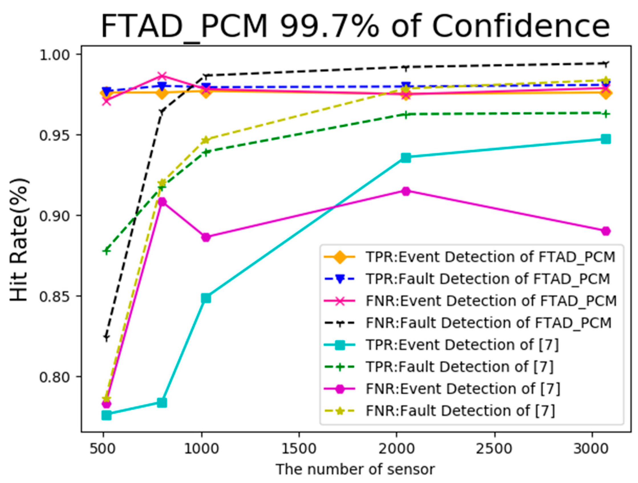
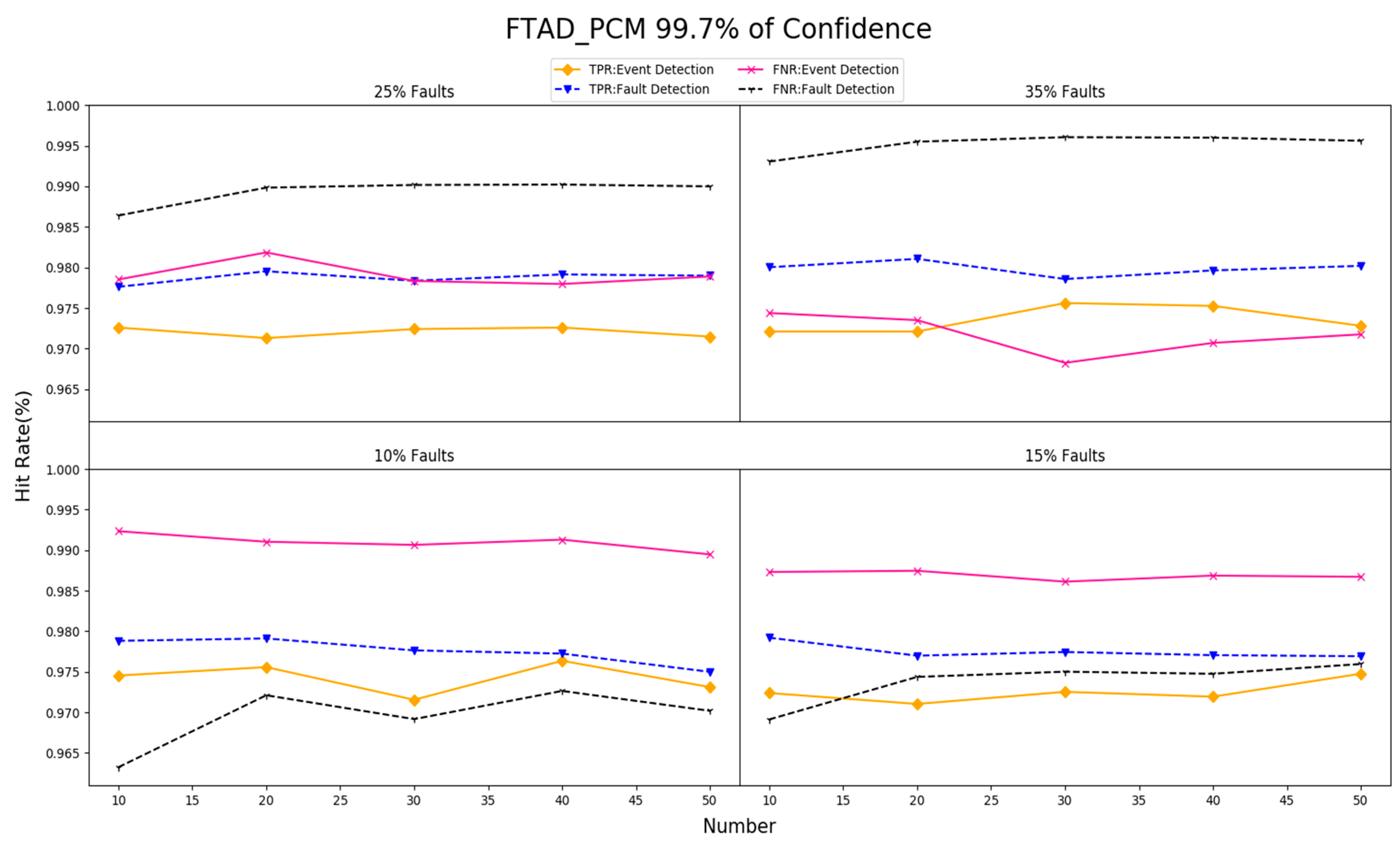
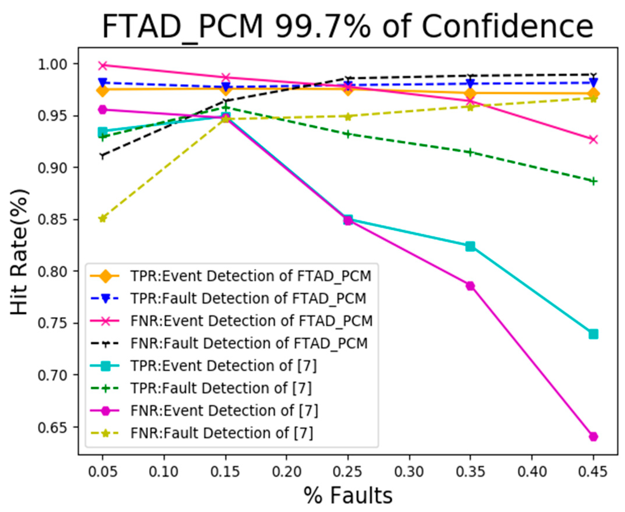
5.2. Result Analysis of Event and Fault Detection

The WSN has 1024 sensor nodes that are deployed randomly in the 32 × 32 space to verify the interval and failure rate of sensor network how to affect our algorithm. In this paper, the sample size k and the failure rate of the sensor network will affect the detection effect, and the results of the experiment are shown in Figure 3. With the increase of the failure rate, the overall TPR of the event decreases, and the FNR increases. The TPR and FNR of the fault are on the rise. This is because the classification of sensor networks into different regions effectively reduces the false alarm rate and increases the hit rate of the faulty nodes. When the failure rate is constant, with the increase of k , the overall hit rate is on the rise. That is, the normal sample interval is closer to the fluctuation interval of the real environment. Considering the limited storage space of sensor nodes, this paper takes k = 40 as a parameter for the follow-up experiment.
In order to verify the performance of our method, we use the simulated data of Table 2 to carry out experiments under different failure rates. We compare with method in [7], using the same simulated data of Table 2 and other parameters from [7]. The network has 1024 sensors. Figure 4 presents the experimental results varying the rate of faulty nodes, with the failure rate of sensor network increasing, the event node TPR and FNR tend to decrease. However, the hit rate of event detection remains at about 97% even with 45% of the sensor nodes failing, and the false positive rate of events being above 92%. Since we consider anomaly detection as both a spatial and temporal correlation, in the temporal correlation part, the state of the node is preliminarily obtained, combined with the spatial correlation to determine the final state of the node. We can also notice a small upward tendency in the faulty node TPR and FNR. This is due to dividing the sensor network into different neighborhoods according to the given network model (Section 3); each of them respectively detects the anomaly in different ways.
In [7], when the failure rate reaches 15%, the TPR and FNR of the event nodes drop rapidly, and the FNR of the faulty nodes increases, but is lower than the method in this paper. This further illustrates the feasibility of combining the spatial-temporal correlation and dividing the sensor networks into different neighborhoods.
Figure 5 presents the experimental results varying the number of sensor node under the 25% of sensors are faulty. Additionally, compared with the method in [7], using the same simulated data of Table 2 and other parameters from [7], the event and faulty TPR and FNR are greatly influenced by the scale of the sensor networks. With the increase of the scale of the sensor networks, they all show an upward tendency. This is because the method of [7] uses most of the principles (Section 4.2), which is greatly influenced by the scale of the sensor network. The FNR of the faulty node in this paper is greatly influenced by the scale of sensor networks, and the greater number of sensor nodes, the lower the false alarm rate. Both the TPR of the faulty node and the TPR, FNR of the event node are maintained in good condition. This is because, for the fault neighborhood, there is a great impact under a low-density sensor network. From the point of view of event detection, this method is also suitable for low-density sensor networks.
Table 3 illustrates the experimental results of the proposed algorithm with comparison to several methods [4,17] under different failure rates. The same simulated data of Table 3 and other parameters are referred to the original paper. The γmin is set to 0.5, c1 is set to 0.1, c2 is set to 0.5 in FDS method. We see that the TPR is decreasing with the fault level. However, the FNR increases as the fault node increases. We observe that the proposed solution guarantees high detection accuracy and low false alarm rate in particular fault node conditions. From Table 3, we can see that our method performs favorably against FDS and KPCA. The reason is that the PCM model can detect anomalies effectively, and divide the sensor network into a given structure (Section 3) to detect faults.

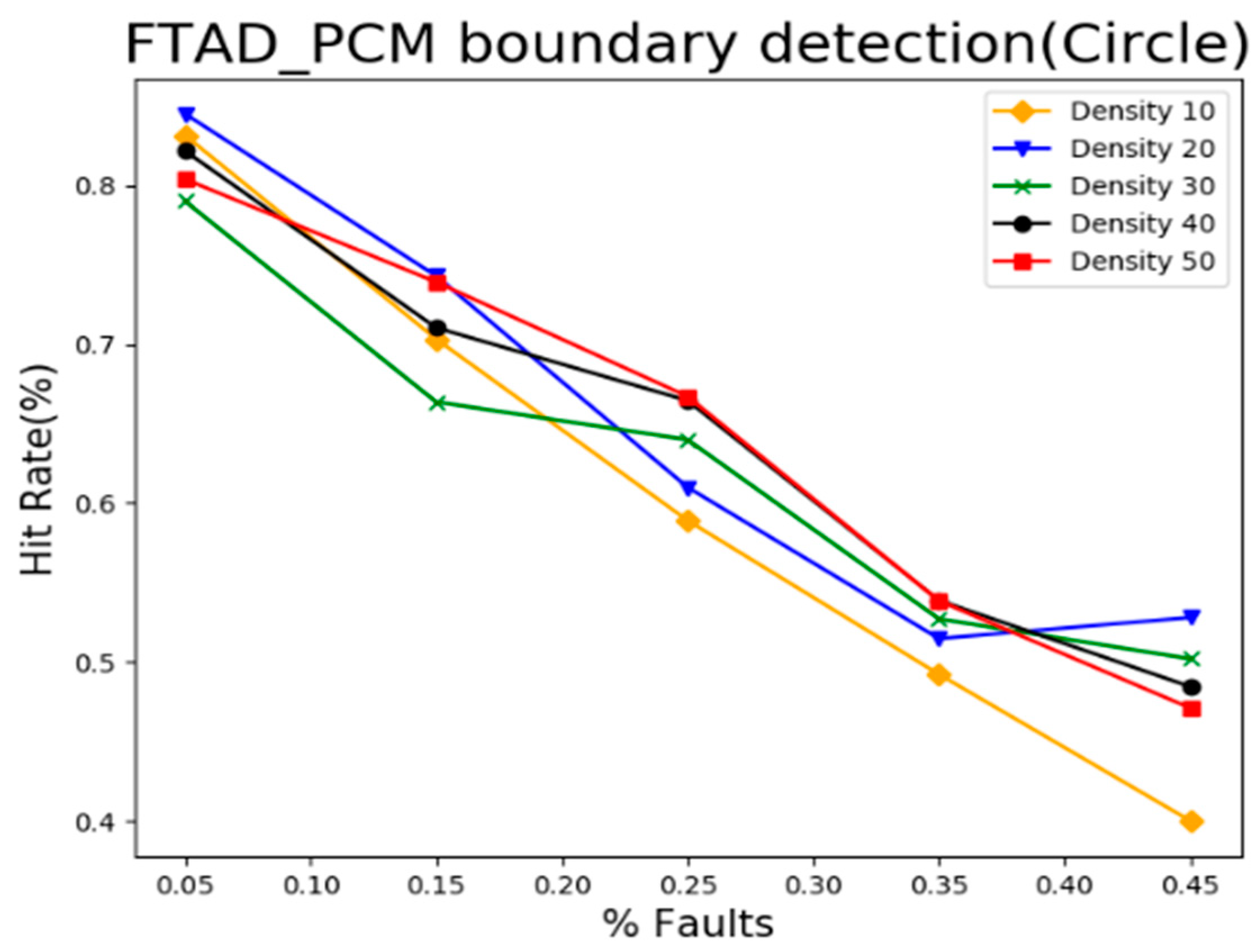
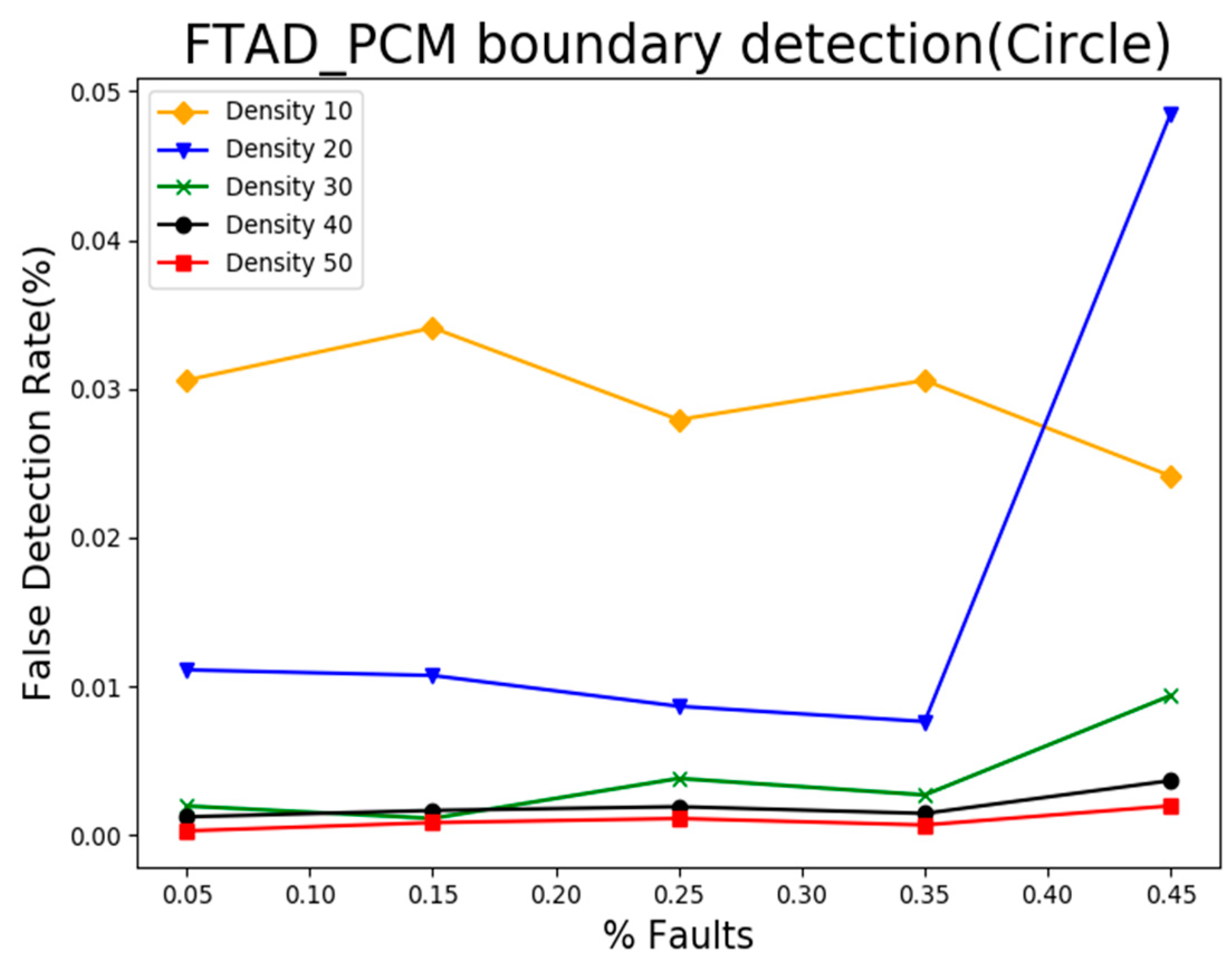
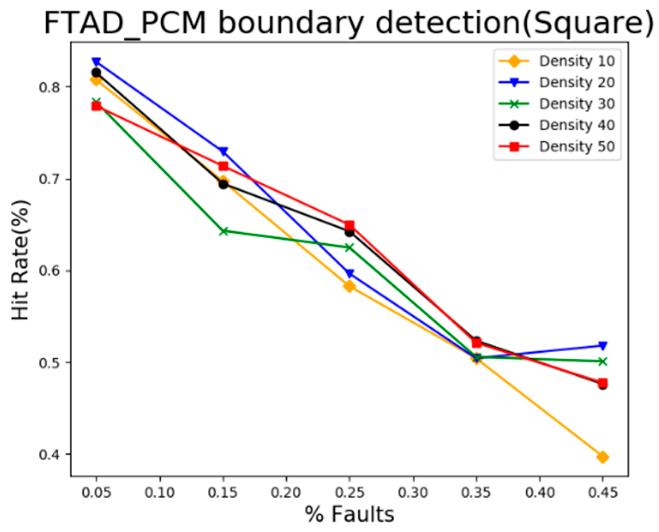
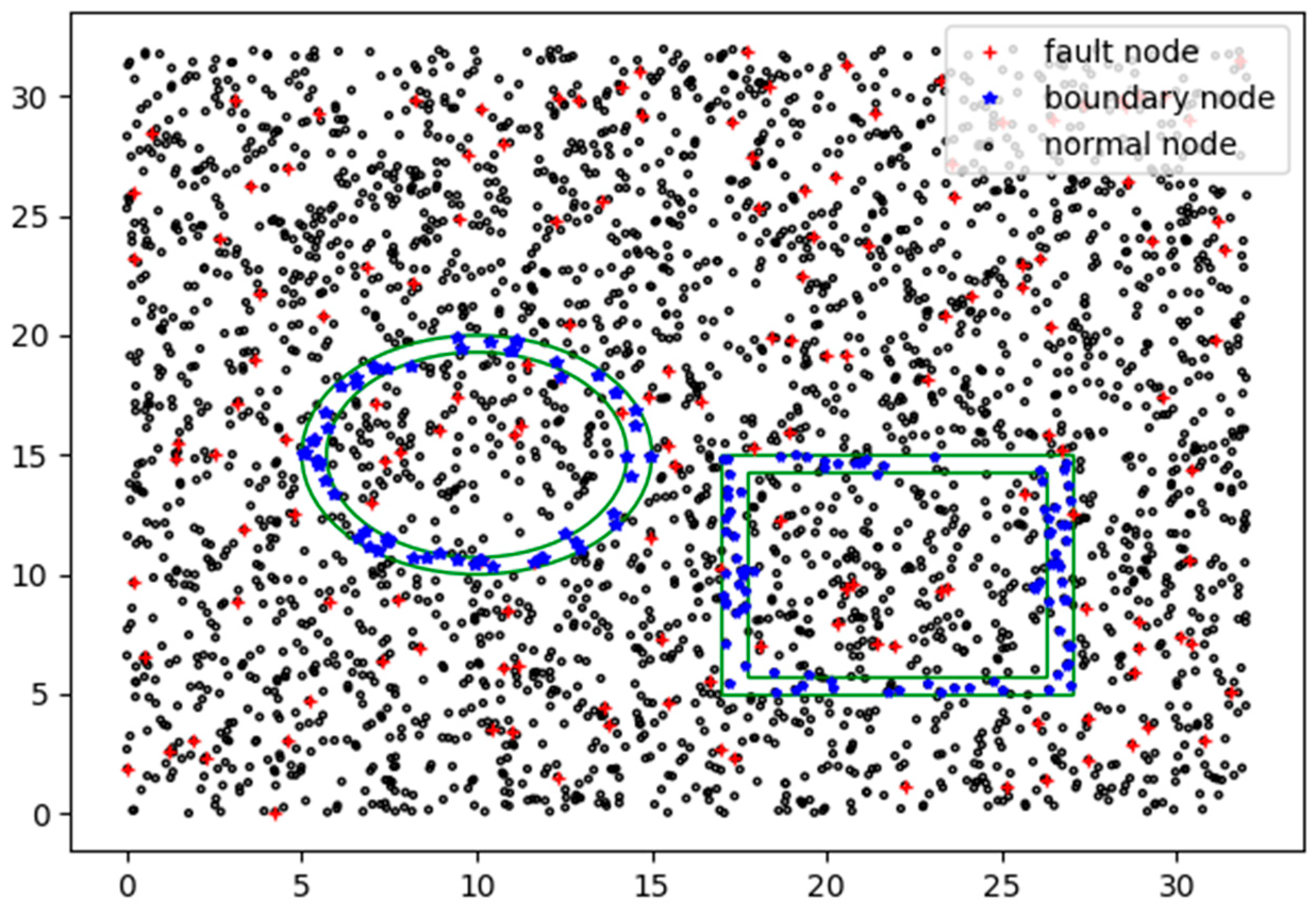
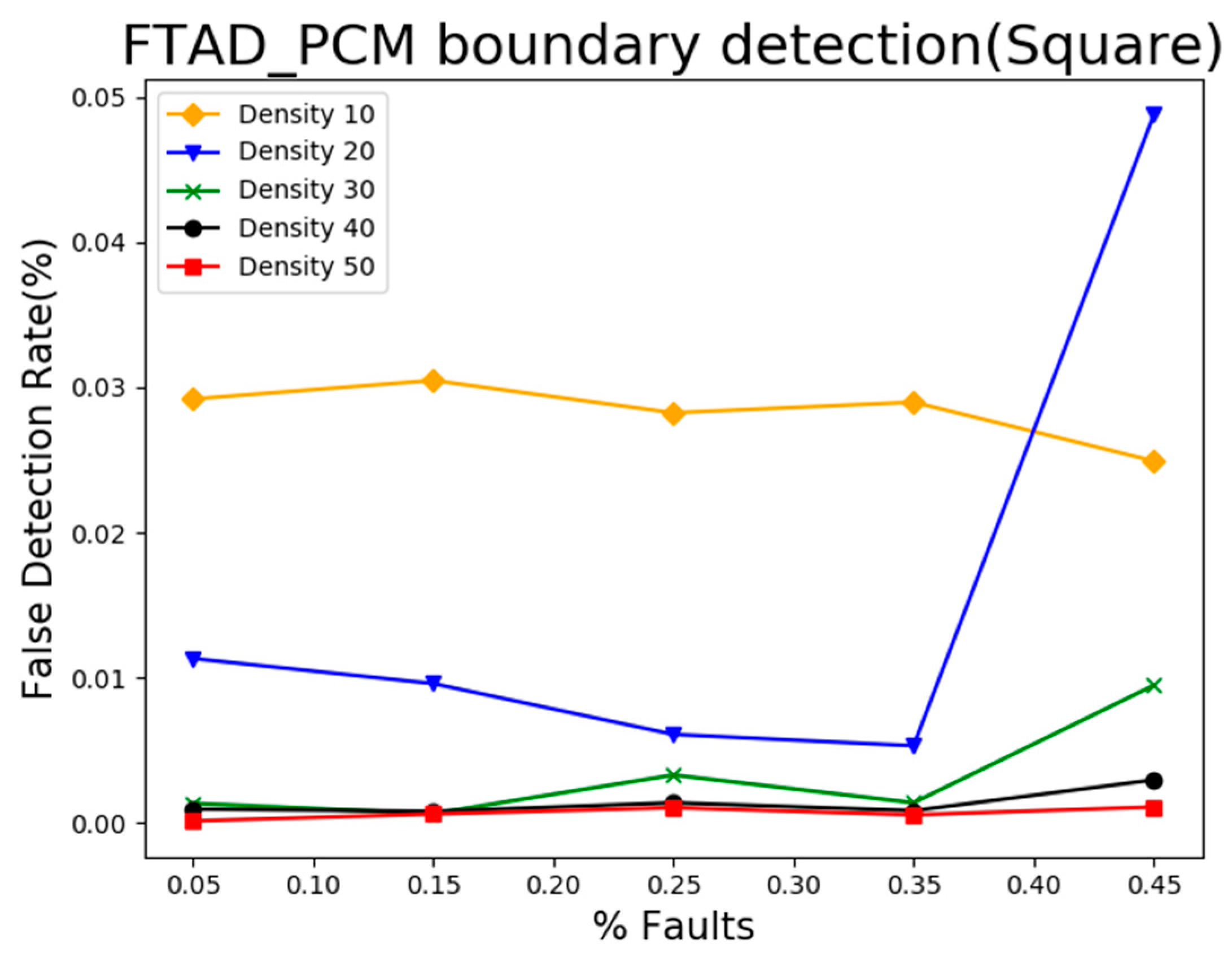
5.3. Result Analysis of Event Boundary Neighborhood Detection

Figure 6 and Figure 7 shows the experimental results of circular event boundaries with different failure rates and sensor network densities. Figure 8 and Figure 9 show the results of the square boundary neighborhood. Both of them use the parameters of Table 2.
From Figure 6 and Figure 8 we can notice that with the increase of the sensor failure rate, the hit rate decreases. When the failure rate is 45%, the average hit rate stays at about 50%, which is acceptable without considering the faulty node as the event boundary neighborhood. The detection results are close given different densities of the sensor network. It shows that the method of detecting the event boundary neighborhood does not depend on the density of the sensor network, and applies to both circular and square event regions.
Figure 7 and Figure 9 are the false detection rate of the boundary neighborhood. With the increase of the sensor failure rate, the false detection rate increases. However, when the failure rate reaches 45%, the false detection rate reaches a low-level, the worst is 0.05%, which shows the validity of the detection in the event boundary neighborhood.
Figure 10 is an experimental snapshot of an event boundary neighborhood. Black “.” represents normal nodes, the red “+” is the faulty node, the blue “*” is the normal node detected as the event boundary neighborhood, and the green circular and square area is the event area. From the graph, we can see that the detected event boundary neighborhood node is located near the boundary of the event area, indicating the effectiveness of the proposed method for event boundary neighborhood detection.

6. Conclusions

In this paper, a spatial-temporal correlation based fault-tolerant event detection method (FTAD) is proposed for event detection in WSNs. Our approach aims at improving the quality of event detection and offering a solution for the problem that the ability of event detection degrades rapidly when the sensor fault probability reaches a critical value. The experiment indicates that FTAD has good performances in high failure rate, and shows that FTAD achieves better performance of event detection than [7]. It has been found that the number of node detecting events is above 97%, and the false negative rates is less than 3.7%, when the sensor fault ratio is 45%. This method is applicable not only to high-density sensor networks, but also to low-density heterogeneous networks. Although this scheme can effectively detect a single event, the performance of the proposed approach in multi-modality event detection needs to be strongly investigated. Future works will be focused on optimizing the proposed method to meet multi-modality event detection in WSNs.

Author Contributions

All authors contributed to writing—original draft preparation and writing—review and editing.

Funding

Funding was provided by the National Natural Science Foundation of China (grant no. 61372107), the Fujian Natural Science Foundation Program (grant no. 2015J05125), and the Huaqiao University graduate research and innovation capacity training program (grant no. 1611422007).

Conflicts of Interest

The authors declare no conflict of interest.

References

  1. Bai, X.; Liu, L.; Cao, M.; Panneerselvam, J.; Sun, Q.; Wang, H. Collaborative Actuation of Wireless Sensor and Actuator Networks for the Agriculture Industry. IEEE Access 2017, 5, 13286–13296. [Google Scholar] [CrossRef]
  2. Qiu, T.; Zhao, A.; Xia, F.; Si, W.; Wu, D.O. ROSE: Robustness Strategy for Scale-Free Wireless Sensor Networks. IEEE/ACM Trans. Netw. 2017, 25, 2944–2959. [Google Scholar] [CrossRef]
  3. Liu, K.; Zhuang, Y.; Liang, J.; Ma, J. Spatiotemporal Correlation Based Fault-Tolerant Event Detection in Wireless Sensor Networks. Int. J. Distrib. Sens. Netw. 2015, 2015, 7. [Google Scholar] [CrossRef]
  4. Alippi, C.; Ntalampiras, S.; Roveri, M. A Cognitive Fault Diagnosis System for Distributed Sensor Networks. IEEE Trans. Neural Netw. Learn. Syst. 2013, 24, 1213–1226. [Google Scholar] [CrossRef] [PubMed]
  5. Osanaiye, O.; Alfa, A.S.; Hancke, G.P. A Statistical Approach to Detect Jamming Attacks in Wireless Sensor Networks. Sensors 2018, 18, 1691. [Google Scholar] [CrossRef] [PubMed]
  6. Sousa, L.D.D.; Frery, A.C.; Nakamura, E.F.; Loureiro, A.A.F. Event detection framework for wireless sensor networks considering data anomaly. In Proceedings of the 2012 IEEE Computers and Communications, Cappadocia, Turkey, 1–4 July 2012; pp. 500–507. [Google Scholar]
  7. Cao, D.L. A Fault-Tolerant Algorithm for Event Region Detection in Wireless Sensor Networks. Chin. J. Comput. 2007, 30, 1770–1776. [Google Scholar]
  8. Lo, C.; Lynch, J.P.; Liu, M. Distributed model-based nonlinear sensor fault diagnosis in wireless sensor networks. Mech. Syst. Signal Process. 2016, 66, 470–484. [Google Scholar] [CrossRef] [Green Version]
  9. Ntalampiras, S. Fault Identification in Distributed Sensor Networks Based on Universal Probabilistic Modeling. IEEE Trans. Neural Netw. Learn. Syst. 2015, 26, 1939–1949. [Google Scholar] [CrossRef] [PubMed]
  10. Tang, P.; Chow, T.W.S. Wireless Sensor-Networks Conditions Monitoring and Fault Diagnosis Using Neighborhood Hidden Conditional Random Field. IEEE Trans. Ind. Inform. 2016, 12, 933–940. [Google Scholar] [CrossRef]
  11. Su, J.; Long, Y.; Qiu, X.; Li, S.; Liu, D. Anomaly Detection of Single Sensors Using OCSVM_KNN. In Proceedings of the International Conference on Big Data Computing and Communications, Taiyuan, China, 1–3 August 2015; Springer: Cham, Germany, 2015; pp. 217–230. [Google Scholar]
  12. Rashid, S.; Akram, U.; Qaisar, S.; Khan, S.H.; Felemban, E. Wireless Sensor Network for Distributed Event Detection Based on Machine Learning. In Proceedings of the 2014 IEEE International Conference on Internet of Things (iThings), and IEEE Green Computing and Communications (GreenCom) and IEEE Cyber, Physical and Social Computing (CPSCom), Taipei, Taiwan, 1–3 September 2014; pp. 540–545. [Google Scholar]
  13. Miao, X.; Liu, Y.; Zhao, H.; Li, C. Distributed Online One-Class Support Vector Machine for Anomaly Detection over Networks. IEEE Trans. Cybern. 2018, 99, 1–14. [Google Scholar] [CrossRef] [PubMed]
  14. Yang, J.; Deng, T.; Sui, R. An Adaptive Weighted One-Class SVM for Robust Outlier Detection. In Proceedings of the 2015 Chinese Intelligent Systems Conference; Springer: Berlin/Heidelberg, Germany; 2016. [Google Scholar]
  15. Swain, R.R.; Khilar, P.M. A fuzzy MLP approach for fault diagnosis in wireless sensor networks. In Proceedings of the 2016 IEEE Region 10 Conference, Singapore, 22–25 November 2016; pp. 3183–3188. [Google Scholar]
  16. Zhao, M.; Tian, Z.; Chow, T.W.S. Fault diagnosis on wireless sensor network using the neighborhood kernel density estimation. Neural Comput. Appl. 2018, 15, 1–12. [Google Scholar] [CrossRef]
  17. Ghorbel, O.; Abid, M.; Snoussi, H. Improved KPCA for outlier detection in Wireless Sensor Networks. In Proceedings of the 2014 1st International Conference on Advanced Technologies for Signal and Image Processing, Sousse, Tunisia, 17–19 March 2014; pp. 507–511. [Google Scholar]
  18. Ding, M.; Chen, D.; Xing, K.; Cheng, X. Localized fault-tolerant event boundary detection in sensor networks. In Proceedings of the IEEE 24th Annual Joint Conference of the IEEE Computer and Communications Societies, Miami, FL, USA, 13–17 March 2005; Volume 2, pp. 902–913. [Google Scholar]
  19. Ali, K.; Ali, S.B.; Naqvi, I.H.; Lodhi, M.A. Distributed Event Identification for WSNs in Non-Stationary Environments. In Proceedings of the IEEE Global Communications Conference, San Diego, CA, USA, 6–10 December 2015; pp. 1–6. [Google Scholar]
  20. Bezdek, J.C.; Havens, T.C.; Keller, J.M.; Leckie, C.; Park, L.; Palaniswami, M.; Rajasegarar, S. Clustering elliptical anomalies in sensor networks. In Proceedings of the IEEE International Conference on Fuzzy Systems, Barcelona, Spain, 18–23 July 2010; pp. 1–8. [Google Scholar]
  21. Ali, K.; Naqvi, I.H. EveTrack: An event localization and tracking scheme for WSNs in dynamic environments. In Proceedings of the 2016 IEEE Wireless Communications and Networking Conference, Doha, Qatar, 3–6 April 2016. [Google Scholar]
  22. Oakland, J. Statistical Process Control; Elsevier: New York, NY, USA, 2008. [Google Scholar]
  23. Krishnamachari, B.; Iyengar, S.S. Efficient and Fault-Tolerant Feature Extraction in Wireless Sensor Networks. In Information Processing in Sensor Networks; Springer: Berlin/Heidelberg, Germany, 2003; pp. 488–501. [Google Scholar]
  24. Ren, K.; Zeng, K.; Lou, W. Secure and Fault-Tolerant Event Boundary Detection in Wireless Sensor Networks. IEEE Trans. Wirel. Commun. 2008, 7, 354–363. [Google Scholar] [CrossRef]
Figure 1. Points a, b, and c are anomaly data with a 0.3% of chance, since they are not in the interval.
Information 09 00236 g001
Figure 2. Architecture of our model for anomaly detection in the WSN.
Information 09 00236 g002
Figure 3. FTAD_PCM with 99.7% confidence.
Information 09 00236 g003
Figure 4. FTAD_PCM detection rate vs. the rate of sensor faults.
Information 09 00236 g004
Figure 5. FTAD_PCM detection rate vs. the number of sensors.
Information 09 00236 g005
Figure 6. FTAD_PCM boundary detection (circle).
Information 09 00236 g006
Figure 7. FTAD_PCM boundary false detection (circle).
Information 09 00236 g007
Figure 8. FTAD_PCM boundary detection (square).
Information 09 00236 g008
Figure 9. FTAD_PCM boundary false detection (square).
Information 09 00236 g009
Figure 10. An experimental snapshot.
Information 09 00236 g010
Table 1. Symbol definition.
SymbolDefinition
n The total number of sensor nodes in the sensor network
T t h Event characteristic duration
Δ T Sensor node adjacent sampling interval
m Times of the sensor node sampled in T t h .
x j i Sampled readings of sensor node S j at time t i
R t h ( t ) The threshold function of sensor reading, in order to determine whether the event occurred
E e ( t ) The expected value of the event
k Sample size
α Confidence
U C L The upper limit (maximum value of normal interval, change with environment)
L C L The lower limit (minimum value of normal interval, change with environment)
L N Sensor node is in the normal condition
L E Sensor node is in the event state
L F Sensor node is in the fault state
F a u l t A fault has occurred on the sensor node
E v e n t The sensor node detected the event
Table 2. Experimental parameters.
ParameterValue
1Sensing area 32 × 32
2Measurement value of the sensor in the event areaNormal distribution ( 100 , 10 )
3Measurement value of the sensor out of the event areaUniform distribution [ 28 , 30 ]
4Faulty measurement value of the sensorUniform distribution [ 30 , 100 ]
5Communication radius 2
Table 3. FTAD vs. KPCA and FDS.
ResultTPRFNR
Method 5%15%25%35%5%15%25%35%
FTAD98.1%98.0%98.0%97.9%91.2%96.0%98.3%98.3%
KPCA95.0%92.5%89.4%85.0%94.0%93.8%91.0%90.0%
FDS97.5%95.3%92.0%88.9%96.5%94.5%92.8%91.1%

