1. Introduction
Microarray is a multiplex technology used in molecular biology and medicine that enables biologists to monitor expression levels of thousands of genes [
1]. Many microarray experiments have been designed to investigate the genetic mechanisms of cancer [
2] and to discover new drug designs in the pharmaceutical industry [
3]. According to the World Health Organization, cancer is among the leading causes of death worldwide accounting for more than 8 million deaths. Therefore, finding a mechanism to discover the genetic expressions that may lead to an abnormal growth of cells is a first order task today. To build a microarray, short sequences of genes tagged with fluorescent materials are printed on a glass surface for hibridization [
4]. Then, the slice is scanned and goes through various data processing steps including image data collection, quality control and normalization. The resulting dataset is a two-dimensional array
with thousands of columns (genes) and several rows (instances):
Every instance (a row in D) is described by a row vector that represents a labeled genetic expression: refers to the expression level of gene , and is the classification for the j-th sample. C may represent different types of cancer or a binary label for cancerous and non-cancerous tissue.
Analysis of microarray data presents unprecedented opportunities and challenges for data mining in areas such as: sample classification and gene selection [
5,
6]. For sample classification, the microarray matrices serve as training sets to a given classifier, to find a classification function
that is able to classify an arbitrary sequence of genes with unknown class from
. Classification function
ℓ is built from analysing the relation between labeled sequence of genes in
D. The performance of supervised classifiers is often measured in three directions: efficiency, representation complexity and accuracy. The efficiency refers to the time required to learn the classification function
ℓ, while the representation complexity often refers to the number of bits used to represent the classification function [
7]. One of the most common metrics to measure the accuracy of a supervised classifier is the error rate defined as:
where
m is the number of sequence of genes in
and
is the complement of the Kronecker’s delta function, which returns 0 if both arguments are equal and 1 otherwise.
The main obstacle in microarray datasets arises from the fact that the genes greatly outnumber the sample observations. As a popular example, in the “Leukemia” dataset, there are only 72 observations of the expression level of 7129 genes [
8]. It is clear that, in this extreme scenario sample, classification methods cannot perform well because of the “curse of dimensionality” phenomena, where excessive features may actually degrade the performance of a classifier if the number of training examples used to build the classifier is relatively small compared to the number of features [
7].
Feature selection plays an essential role in microarray data classification since its main goal is to identify and remove irrelevant and redundant genes that do not contribute to minimize the error of a given classifier [
9]. Basically, the advantages of feature selection include selecting a set of genes
with:
where
is the result of projecting
over
D. In addition, when a small number of genes are selected, their biological relationship with the target diseases is more easily identified. These “marker” genes thus provide additional scientific understanding of the causes of the disease [
6]. Feature selection plays a fundamental role for increasing efficiency and enhancing the comprehensibility of the results.
In gene selection, genes are evaluated based on (i) their individual relevance to the target class, (ii) the redundancy level respect to other genes, and (iii) how the gene interacts to other genes [
10]. The relevance and the redundancy level of a gene are often measured by correlation coefficients such as: Pearson’s correlation [
11], Mutual Information (
MI) [
12], Symmetrical Uncertainty [
13] and others. On the other hand, it is said that a gene interacts with other genes if, when combined, it becomes more relevant [
14]. Most of the feature selection algorithms in the literature evaluate features by only using one or two of these aspects, but not using all three of them as a whole. This may lead the algorithm to output low-quality solutions, especially when redundant genes and interacting genes are abundant in the problem. In addition, we have detected that most of feature selection algorithms in the literature suffer from what we call the
integrality problem (to be defined). Roughly speaking, the
integrality problem occurs when the relevance of a gene is measured by the average of the correlation of their values with the target class. We will further analyse this problem in
Section 3.
While not losing sight of the fact that microarray cancer datasets are large and abundant in “noisy” genes, the first goal of this paper is to present a new algorithm able to efficiently detect and select relevant, non-redundant and interacting genes to improve the accuracy of classification algorithms. In order to reach this task:
We first introduce a new feature selection methodology that can avoid the integrality problem.
Second, we present a new simple algorithm that can detect irrelevant, redundant and interacting genes in an efficient way.
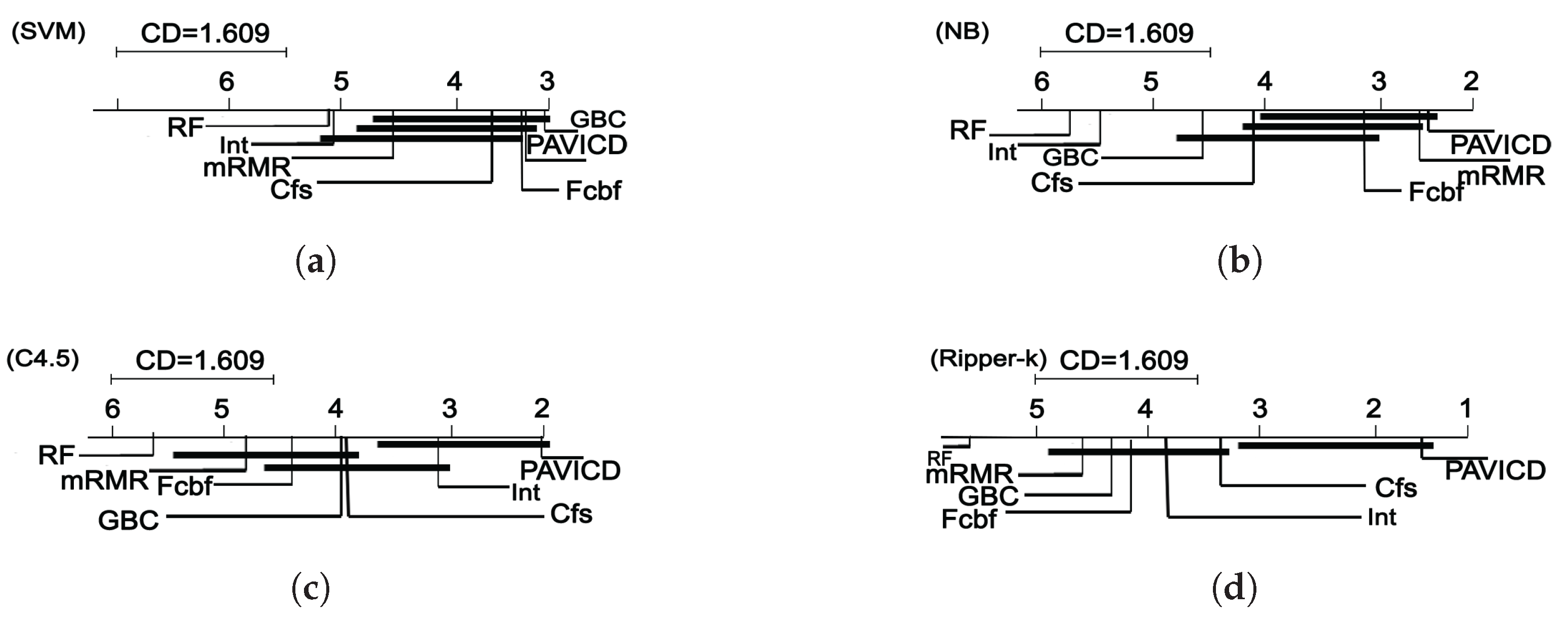
Finally, the new algorithm is compared with five state-of-the-art feature selection algorithms in fourteen microarray datasets, which include leukemia, ovarian, lymphoma, breast and other cancer data.
3. Materials and Methods
In this section, we introduce a new methodology to create feature selection algorithms that take advantage of feature value information to avoid the
integrality problem mentioned in
Section 1. For a better understanding of the
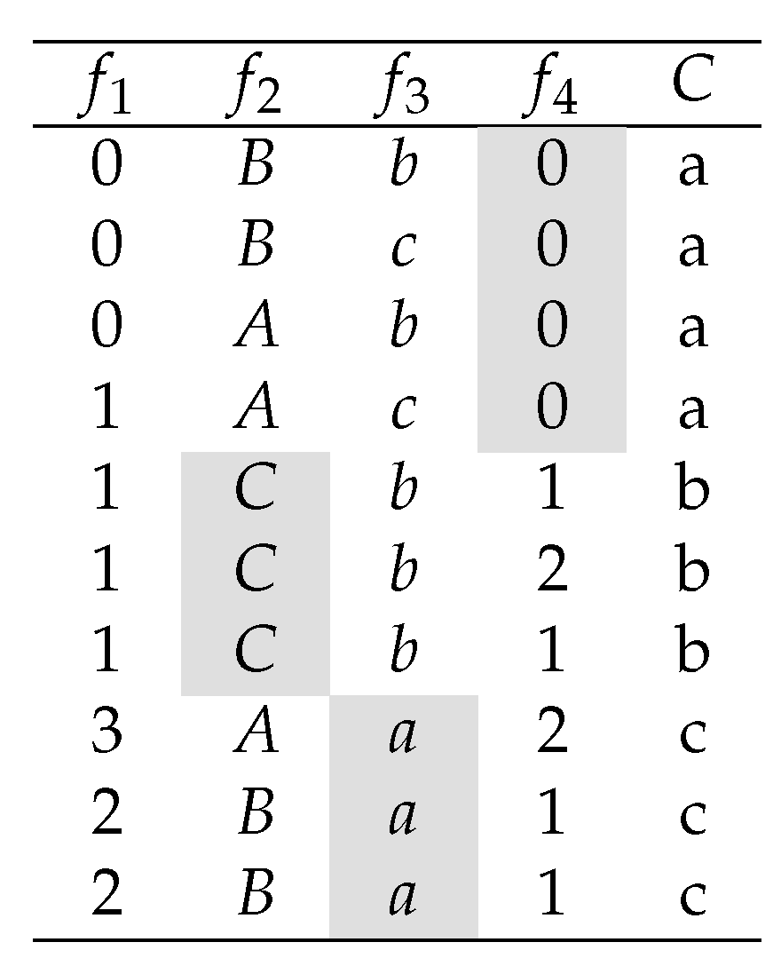
integrality problem, consider the dataset depicted in
Figure 2.
Note that the
Symmetrical Uncertainty of
,
,
and
with respect to class
C is
,
,
and
respectively. Therefore, most of the feature selection algorithms described in
Section 2, will select
as the best feature, and the rest of the features might be selected or not according to their correlation (redundancy score) with
. However, it is clear that class
C is perfectly predictable by three one-precedent rules when
is selected.
This problem occurs because features in have at least one value that is highly correlated with a class label and its other values are not correlated with the class. Consequently, if the relevance of these features (genes) is measured by averaging the prediction power of all its feature values, then this feature may be considered irrelevant. We call this phenomena the integrality problem. Note that we call the correlation of a feature value with respect to a class label of C, to the existing correlation between the binary feature obtained from the respective feature and a given class label. As an example, the feature value of feature is . Note that the correlation between and the target class C, given that , is maximal.
3.2. Pavicd: A Probabilistic Rule-Based Algorithm
We now introduce a new algorithm, namely Pavicd (Probabilistic Attribute-Value Integration for Class Distinction), which is based on the methodology aforementioned. In order to develop the algorithm, we take into account three aspects: first, how to deal with non-binary datasets, second, how to build for each class label , and third, to develop functions to measure the relevance, redundancy and interaction score of feature values.
The first step in Pavicd is the preparation of data. Since the proposed methodology is based on the evaluation of feature values, instead of features, dealing with non-binary data can be difficult. However, to deal with non-binary data, Pavicd builds a new space of binary features through the decomposition of each feature in (v number of feature values of ) new binary features where each one of them take value “1” in the position, where the respective feature value appears in the original feature and takes value “0” in the other positions. Note that this conversion is reversible because the original feature could be obtained through the union of its binary features. With this transformation, a feature is analysed piecemeal, so that its most intrinsic useful information to predict a given class label is easily identified.
The second step is to determine, and store in which of the entire sets of feature values are relevant for a given class label . Here, we adopt a very simple approach that consists of selecting the covering or reliable feature values for a given class label . Note that we use two thresholds, namely and , to fix the lower bound value for the selection of covering and reliable values, respectively.
Definition 1. A feature value is said to be covering with respect to the class label if and .
Definition 1 suggests that a feature value is covering with respect to the class if the conditional probability of given is the largest among all the class labels in C. Note that all features values in are covering for at least one class label. Therefore, we use the threshold to discriminate between “good” covering values and "bad" covering values for a given class label.
Definition 2. A feature value is said to be reliable with respect to the class label if and .
According to Definition 2, a feature value is likely to be reliable for a given class if it occurs many times in and almost does not occur in the rest of the class labels. Note that, again, we introduce a new threshold to filter the feature values.
In the third step, we carried out the Integration Analysis by means of a
sequential forward search. The
sequential forward search is twofold. First, the best feature value in
is identified and included in the current solution set
; and second, the
sequential forward search itself is performed. To select the best feature value in
, we use the following evaluation function:
This measure is equal to 1 when
completely covers
and does not occur in any other instance with different class (as
feature values ,
and
in the example of
Figure 2), and it takes value 0 if the feature value does not occur in any of the instances labelled with class
. In other words, we may expect that the best
feature value is a highly-covering and highly-reliable one. For the
sequential forward search, we start with
equal to the
feature value in
that maximizes Equation (
7), and, then, in each iteration, we explore
so that
feature value that maximizes
is selected, and
feature value such that
holds, is removed from
and never tested again. Note that, since Pavicd deals with binary features (or
feature values), the current solution
is also a binary feature because it is the result of one of “AND” or “OR” operators between two binary features. This is briefly explained below.
To evaluate how good a feature value is with respect to the already selected set , we use the following set of rules:
Rule 1. If both and are covering feature values, then
Rule 2. If both and are reliable feature values, then
Rule 3. If neither Rule 1 or Rule 2 hold, then apply the Rule (1 or 2) that maximizes .
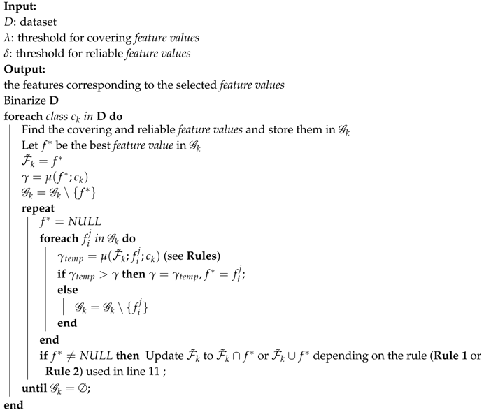
Note that is treated as a feature value (or a binary feature) because every time a feature value is “added” to , is transformed to or if Rule 1 or Rule 2 holds, respectively. Algorithm 1 shows the pseudo code of Pavicd.
| Algorithm 1: Algorithm of Pavicd |
![Information 09 00006 i001]() |


