Article

A Comparison Study of Kernel Functions in the Support Vector Machine and Its Application for Termite Detection

by
Muhammad Achirul Nanda
1,
Kudang Boro Seminar
1,*,
Dodi Nandika
2 and
Akhiruddin Maddu
3
1
Faculty of Agricultural Technology, Bogor Agricultural University, Bogor 16680, West Java, Indonesia
2
Faculty of Forestry, Bogor Agricultural University, Bogor 16680, West Java, Indonesia
3
Faculty of Mathematics and Natural Sciences, Bogor Agricultural University, Bogor 16680, West Java, Indonesia
*
Author to whom correspondence should be addressed.
Information 2018, 9(1), 5; https://doi.org/10.3390/info9010005
Submission received: 10 December 2017 / Revised: 27 December 2017 / Accepted: 28 December 2017 / Published: 2 January 2018

Abstract

:
Termites are the most destructive pests and their attacks significantly impact the quality of wooden buildings. Due to their cryptic behavior, it is rarely apparent from visual observation that a termite infestation is active and that wood damage is occurring. Based on the phenomenon of acoustic signals generated by termites when attacking wood, we proposed a practical framework to detect termites nondestructively, i.e., by using the acoustic signals extraction. This method has the pros to maintain the quality of wood products and prevent higher termite attacks. In this work, we inserted 220 subterranean termites into a pine wood for feeding activity and monitored its acoustic signal. The two acoustic features (i.e., energy and entropy) derived from the time domain were used for this study’s analysis. Furthermore, the support vector machine (SVM) algorithm with different kernel functions (i.e., linear, radial basis function, sigmoid and polynomial) were employed to recognize the termites’ acoustic signal. In addition, the area under a receiver operating characteristic curve (AUC) was also adopted to analyze and improve the performance results. Based on the numerical analysis, the SVM with polynomial kernel function achieves the best classification accuracy of 0.9188.

Graphical Abstract

1. Introduction

Living in large underground colonies, termites can attack any wood that has a direct contact to the ground and can even lead to the death of a healthy tree. Termites are harmful pests that economically impact the quality of the wood in wooden buildings, forest trees and crops. As can be seen in Figure 1, it shows the initial attack of subterranean termites on Acacia crassicarpa plantation, Riau Province, Indonesia. In addition, the damage of wooden buildings by termites is also easy to find in Bogor city and surrounding areas [1]. In fact, some areas of the important buildings in Indonesia have been seriously attacked e.g., Presidential Palace, Istana Merdeka, Jakarta, etc. [1]. Nandika et al. [2] reported that the cost, due to termite attacks to wooden buildings, was estimated to reach about Rp 8.7 trillion in 2015 not including treatment costs, repairs of the damaged buildings and loss of property value. Approximately 2500 termites species exist worldwide and about 300 species are considered pests [3]; the most wooden building attacks in Indonesia are caused by subterranean termites in the genus Coptotermes (Isoptera: Rhinotermitidae), species Coptotermes curvignathus.
To overcome termite attacks and avoid a higher wood damage, a detection system is required for the inspection process. So far, two methods have been developed, namely visual and non-visual inspection. The visual inspection requires to one open the wood directly, which becomes the most dominant method used nowadays [4]. Hence, it leads to damage in the wood structure. In addition, in terms of inspection efficiency, so far there is no scientific report that tested this method [4]. Conversely, the non-visual inspection becomes the attractive solution because it is a non-destructive method, where the wooden structure remains intact. Nowadays, many detection systems are extensively applying the non-visual method, which may include an electronics stethoscope [4], methane gas odor [5], moisture meter and acoustic emission [6,7].
In a state of the art study of termite detection, based on the acoustic signal, Lewis et al. [8] analyzed the performance of the termite detection tool (wood-destroying insect detector®, DowAgrosciences, Indianapolis, IN, USA) and obtained the detection accuracy result of 89.45%. Lewis used the western drywood termite, Incitermes minor (Hagen) for his research. Since, the most massive termite attacks in Indonesia come from subterranean termites, Coptotermes curvignathus, this study focused on the termite detection system using Coptotermes curvignathus.
The acoustic from insects often produce signals with spectral and temporal features that make them distinctive and easily detectable [9]. The acoustic signals generated by termites become a basic standard to design a termite detection system. Some researchers reported that specific activity, namely eating, excavation and head-banging would generate the particular acoustic signal [10,11]. Over the last decade, the application of microphones has been successful to detect insects within wood [12,13,14] and to solve various engineering problems [15,16,17,18,19]. Therefore, in this study, we used the microphone electret sensor to sense the acoustic signal produced by termites.
The core problem in developing a termite detection system is to separate the signals generated by termites and background noise [20]. The proposed alternative to address this problem is to build a reliable classification model. In this study, we apply the support vector machine (SVM) algorithm. This is a new approach implemented into our system, because so far, no scientific report has been reviewed about this work. Please note that some significant advantages of using this algorithm are high accuracy, direct geometric interpretation and elegant mathematical tractability [21]. In addition, the SVM does not require a large number of training data set to avoid the overfitting issues. In the process of developing a classification model using SVM, the kernel function plays a significant role because it assists in mapping dataset to a higher dimensional space to obtain a better interpretation at the classification model. However, in fact, there are many types of kernel functions that can be applied such as linear, radial basis function, sigmoid and polynomial. This study will investigate the comparison of several kernel functions used at the SVM algorithm to achieve the best result performance in the termite detection system.
The rest of the paper is organized as follows: Section 2 discusses the materials and methods involved: the description of monitoring and feature extraction on acoustic signals, various types of kernel function in SVM, and performance evaluation with analysis of receiver operating characteristics (ROC). Section 3 details acoustic signal characteristics and parameter optimization on kernel function with grid-search method. Section 4 gives the data processing results obtained from the implemented algorithm in the termite detection system. Finally, Section 5 shows our main conclusions.

2. Materials and Methods

2.1. Selection of Boards

Pine wood (Pinus merkusii) was selected as the experimental sample of the board with the initial moisture content of 8.75 ± 0.05%. The board has the dimensional size (20 × 9.5 × 2.5 cm) and the inside has a hole with size (12 × 6 × 0.5 cm). The groups of the boards were divided into two classes i.e., infested class and uninfested class. The infested class has 220 subterranean termites (i.e., 200 workers and 20 soldiers) inserted into a board, while the uninfested class does not include any termite into a board and serves as the control. Each class includes a total of five boards; for example, the infested class and uninfested class use a total of five boards for the measurement process respectively. The selection of wood species and the number of termite populations refer to Indonesia standard (SNI 2006) [22]. This standard testing to detect the existence of termite attacks through its acoustics was completed at Termite Laboratory, Bogor Agricultural University, 28 °C, 70% RH, in the dark room for 2 weeks before the acoustic signal acquisition.

2.2. Acoustic Signal Monitoring

First, we used two electret microphones (Itead studio, Shenzhen, China) placed on the wood for sensing termite acoustic signals. This sensor has a frequency range of 0.1–10 kHz and a sensitivity of −50 dB. Furthermore, it is connected with a microcontroller to convert acoustic signals into an equivalent electrical voltage. This signal is displayed and analyzed using the software of R studio, Inc. (version: 0.99.896-©2009-2016, Boston, MA, USA) on computer (ThinkPad X-240) with 2.49 GHz Intel® Core™ i5 CPU, 64-bit operating system, and 8 GB RAM.
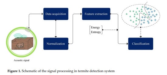
As can be seen in Figure 2, it shows the schematic diagram of our termite detection system. Initially, each wood in two groups (infested and uninfested class) had its acoustic signal measured 10 times. The data acquisition process was digitized at a 100 Hz sampling rate for 3 s and the signal was normalized using the following equation [23]:
N [ i ] = x [ i ] x [ max ]
where, N [ i ] is the normalization results of the data-i, x [ i ] is the data value, x [ max ] is the maximum value of the entire data.
The next stage is the feature extraction, which is a process of reducing the data to produce the features that describe the characteristics of the observation object in order to avoid the complex computation. In this paper, we propose using the two features: energy and entropy. Energy ( E ( i ) ) is described as the sum of squares of the amplitude (value of acoustic signal) in the length of signal. This is defined as follows [24]:
E ( i ) = 1 w L n = 1 w L | x i ( n ) | 2
where, w L is the length of the acoustic signal, n = 1, …, w L , and x i is defined as a value of the acoustic signal. Whereas, entropy (H) is depicted as a measure of abrupt changes in the energy level from the acoustic signal. This can be calculated using Equation (3) [24,25], where, e j is the ratio of the total energy of the sub-length acoustic signal to the total energy of the entire acoustic signal.
H = e j   log 2 ( e j )
Both of the proposed features are obtained in the time domain. It means that the features are extracted directly from the data results generated by the electret sensor without requiring a signal transformation. Furthermore, at the classification stage, the feature extraction result is used for the input to build the classification model. In this study, we implemented a support vector machine (SVM) algorithm to recognize the termite acoustic characteristics. The explanation of SVM implementation into our system is given in Section 2.3.

2.3. Support Vector Machine Classifier

There are numerous artificial intelligence factors based on supervised learning algorithms [26] which can be applied to detect acoustic signals. An SVM classifier is applied in the current detection framework, due to its outstanding generalization capability and reputation in the training data set to achieve high accuracy [27,28,29]. This method is based on statistical learning theory and structural risk minimization principle. The strategy of this classifier is to find an optimal separating hyperplane with the maximum margin between the classes by focusing on the training samples located at the edge of the class distribution [30]. As a very effective method for pattern recognition, SVM proposed by Vapnik, has characteristics which are [31]: (1) SVM can be generalized in a high-dimensional space with a small sample of training only; (2) The optimum result can be given through transformation into a quadratic programming; (3) SVM can simulate nonlinear functional relationships.
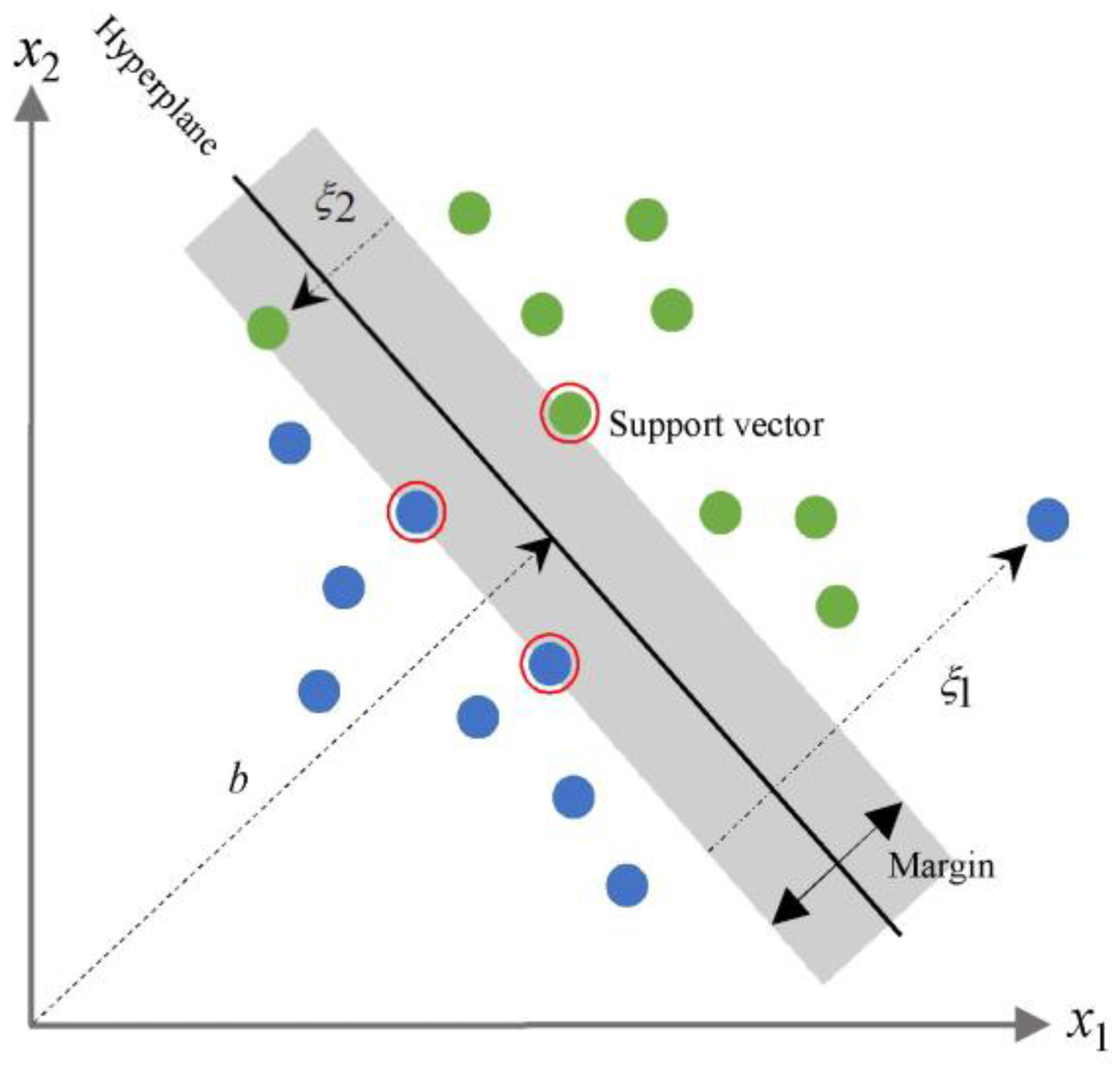
A brief description of SVM is illustrated below. In binary classification problem with linearly separable (Figure 3), has a goal to find the optimum hyperplane, through maximizing the margin and minimizing the classification error between each class y i { + 1 ,   1 } from x-dimensional input data. In this case of termite detection system, x i represents the features extraction in acoustic signal, i.e., energy and entropy, while y i labels the infested class ( + 1 , green color) and uninfested class ( 1 , blue color) (Figure 3). This hyperplane can be described in Equation (4), where, w is normal a vector of the hyperplane and b is described as the position of the relative area to the coordinate center.
w . x i + b = 0
The optimization of this margin to its support vector can be converted into a constrained quadratic programming problem as seen in Equation (5) [32]. Where, ξ i is the slack variable which represents the misclassified sample of the corresponding margin hyperplane, parameter C represents the cost of the penalty. If C is too large, then error minimization is predominant. Otherwise, if C is too small, then margin maximization is emphasized.
{ min 1 2 w 2 + C i = 1 n ξ i s . t . y i ( w T x i + b ) 1 ξ i ξ i 0

2.4. Kernel Function

One of the obstacles in the classification process is the dispersion of data tending diversely, so it will be difficult to be separated linearly [33,34]. In this case, SVM introduces the kernel function [35], K ( x n , x i ) , which transforms the original data space into a new space with a higher dimension; this process includes the transformation function with dot product ϕ ( x ) (Equation (6)). The aim is the data, which already transformed into a higher dimension, can be separated easily. Thus the hyperplane function can be written in Equation (7).
K ( x n , x i ) = ϕ ( x n ) ϕ ( x i )
f ( x i ) = n = 1 N α n y n K ( x n , x i ) + b
where, x n is support vector data, α n is lagrange multiplier and y n is the label of membership class ( + 1 , 1 ) with n = 1, 2, 3, …, N. In this study, we investigate the comparison of using the four kernel functions at the SVM algorithm, i.e., linear, radial basis function (RBF), sigmoid and polynomial, which are listed in Table 1. Each kernel function has a particular parameter that must be optimized to obtain the best result performance [21].
The core of this stage is to analyze the optimal value of the parameter (i.e., C ,   γ ,   r , and d) for each kernel, so the unknown data can accurately be predicted by the classifier. In this study, we use the grid-search method for tuning parameters at the kernel function. In the grid-search method, firstly, we set the appropriate values in the region of the grid for the upper and lower bounds as follows: C   ( 2 15 ,   2 14 ,   ,   2 2 ) , γ   ( 2 10 ,   2 9 ,   ,   2 2 ) , r   ( 2 10 ,   2 9 ,   ,   2 2 ) , and d   ( 0 ,   1 ,   2 ,   3 ) . This method works by searching the combination of the parameters in the given length of region, then issuing the best parameter value based on the minimum classification error to build the classification model. In addition, in this study, this method offers the accuracy with 10-fold cross validation in the training data set. The grid-search is straightforward, but seems naive. The reasons why we use this method are as follows: (1) Psychologically, we may not feel safe to use approximation methods or heuristics, which perform extensive parameter search; (2) The computational time to find the optimal parameter values by the grid-search is not much more than those by advanced methods [37]; (3) The grid-search can be easily parallelized because each pair is independent [38]. In addition, the grid-search is kind of an iterative method and as we know, many advanced algorithms are based on iterative processes.

2.5. Classifier Evaluation

Before making any predictions on whether the wood is infested by termites or not, we need to train the data set containing the characteristics corresponding to the experimental samples of the known class. Next, with the same data set, we evaluate the performance of the classification models. In this study, we used the receiver operating characteristics (ROC) curve for the evaluation process. A ROC curve depicts relative trade-offs between sensitivity or true positive rate ( T P r a t e ) as the y coordinate and 1-specificity or false positive rate ( F P r a t e ) as the x coordinate; it is useful in assigning the best cut-offs for classification [39]. The most common quantitative index for describing the accuracy is expressed by area under the ROC curve (AUC), which provides a useful parameter for assessing and comparing classifier. The calculation of AUC includes the results from f ( x i ) (Equation (7)) in training data set with different kernel function. Furthermore, the AUC can be determined in Equation (8) and Table 2 summarizes the accuracy’s grading system in AUC.
AUC = 1 + T P r a t e F P r a t e 2
The area under the ROC curve (AUC) is a better tool for visualizing and evaluating classifiers than scalar measures such as accuracy, error rate or error cost [40,41]. The advantage of this curve is to enable visualizing and organizing classifier performance without regard to class distributions or error costs. This characteristic becomes very important when investigating a learning with skewed distributions or cost-sensitive learning. According to Bradley [42], the ROC curve offers some desirable properties to measure the classification performance, i.e., it indicates how well separated the negative and positive classes are for the decision index.

3. Results

3.1. Acoustic Signal Dispersion

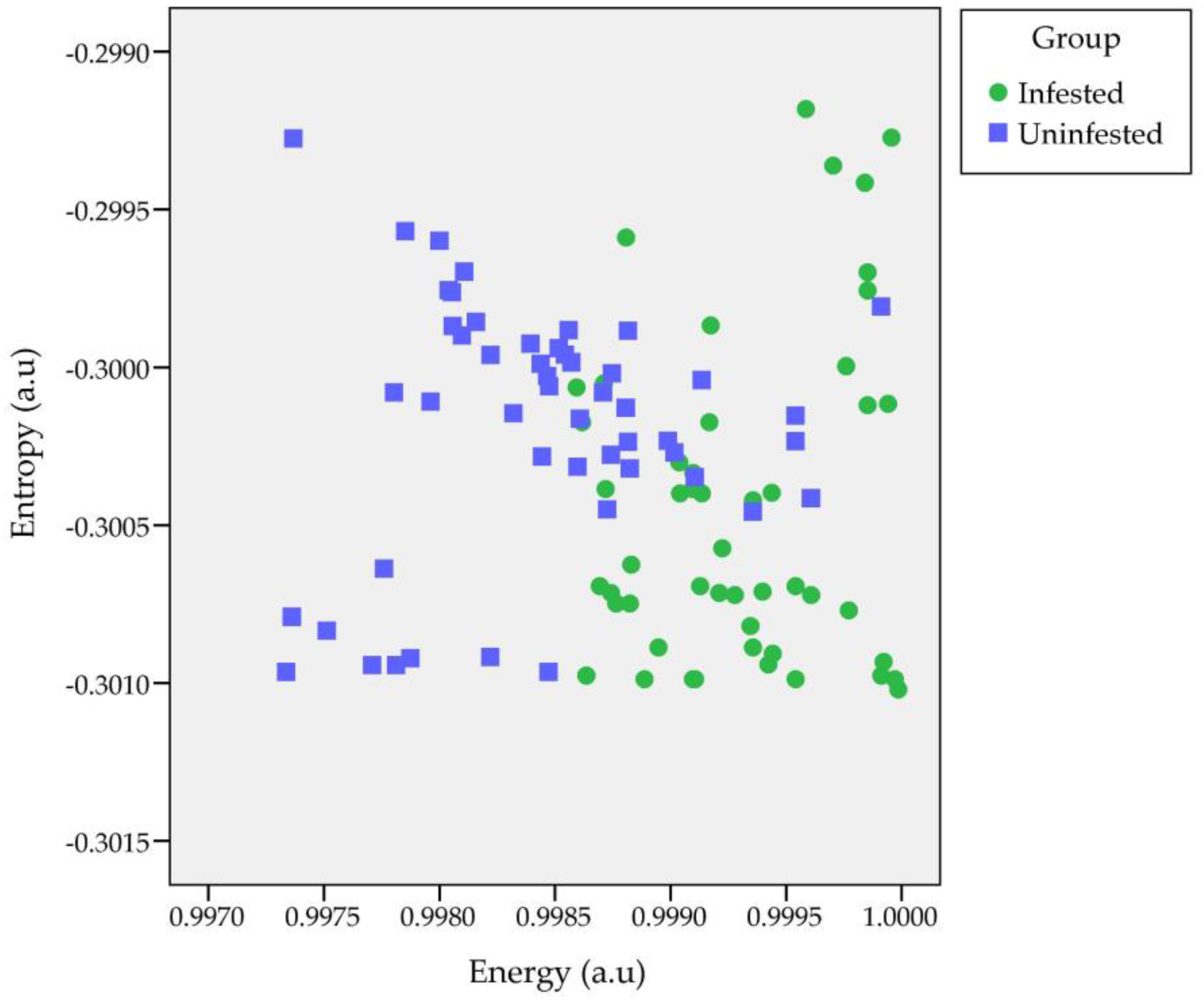
Figure 4, based on experiment results, shows two dimensional (2D) plots of the features extraction from acoustic signal acquisition for the two groups, i.e., the infested and uninfested group. Visually, the data dispersions in both groups are difficult to be separated if we apply the linearly separable hyperplane, because it will lead to overlapping issues; of course, it will have an impact on errors in the classification process. In such a case, a kernel function is required to transform the data into a higher dimensional space, so the acoustic signal characteristics in both groups can easily be separated.

3.2. Grid-Search Optimization

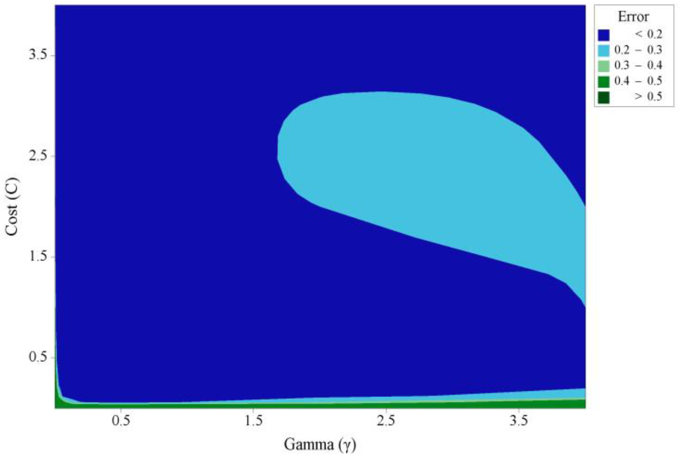
In this section, the critical process presents the grid-search methods for the parameter optimization in each kernel function. First, the experiments were completed with package e1071 in R studio software. To build the optimal hyperplane model, we used the total numbers of 50 data sets in each class for a training process that includes two feature extractions i.e., entropy and energy. To visualize how the grid-search is employed, we give one example of a kernel that has two parameters (C and γ ) for the optimization, i.e., RBF. Its graphical display is shown in Figure 5. As mentioned, based on 10-fold cross validation results, the grid-search successfully finds the optimal pair of the both parameters located in the blue zone (with error <0.2, exactly 0.15); it has the combination parameters of C = 2 1 and γ = 2 3 respectively.
The overall summary of the various kernels is listed in Table 3. It can be seen that the best hyperplane model is owned by the polynomial kernel function. The reason is that this kernel has the lowest classification error of its competitors (linear, RBF and sigmoid). Meanwhile, the kernel that has the highest classification error is the linear kernel function.
The predetermined upper and lower bounds (Section 2.4) with the grid-search method were a success in issuing optimal pair value (Table 3). This is significantly useful for developing a classification model. However, please note that the setting of search interval is a problem. Too large a search region will waste the computational resource. This happens when searching the optimal pair value on polynomial kernel that requires computation time is relatively longer than other kernels, since this kernel has four parameters that are necessary to be optimized. While, if too small, a search region might render a satisfactory outcome impossible [43]. Therefore, we have precisely analyzed the search region first before performing the optimization simulation.

3.3. Performance Evaluation

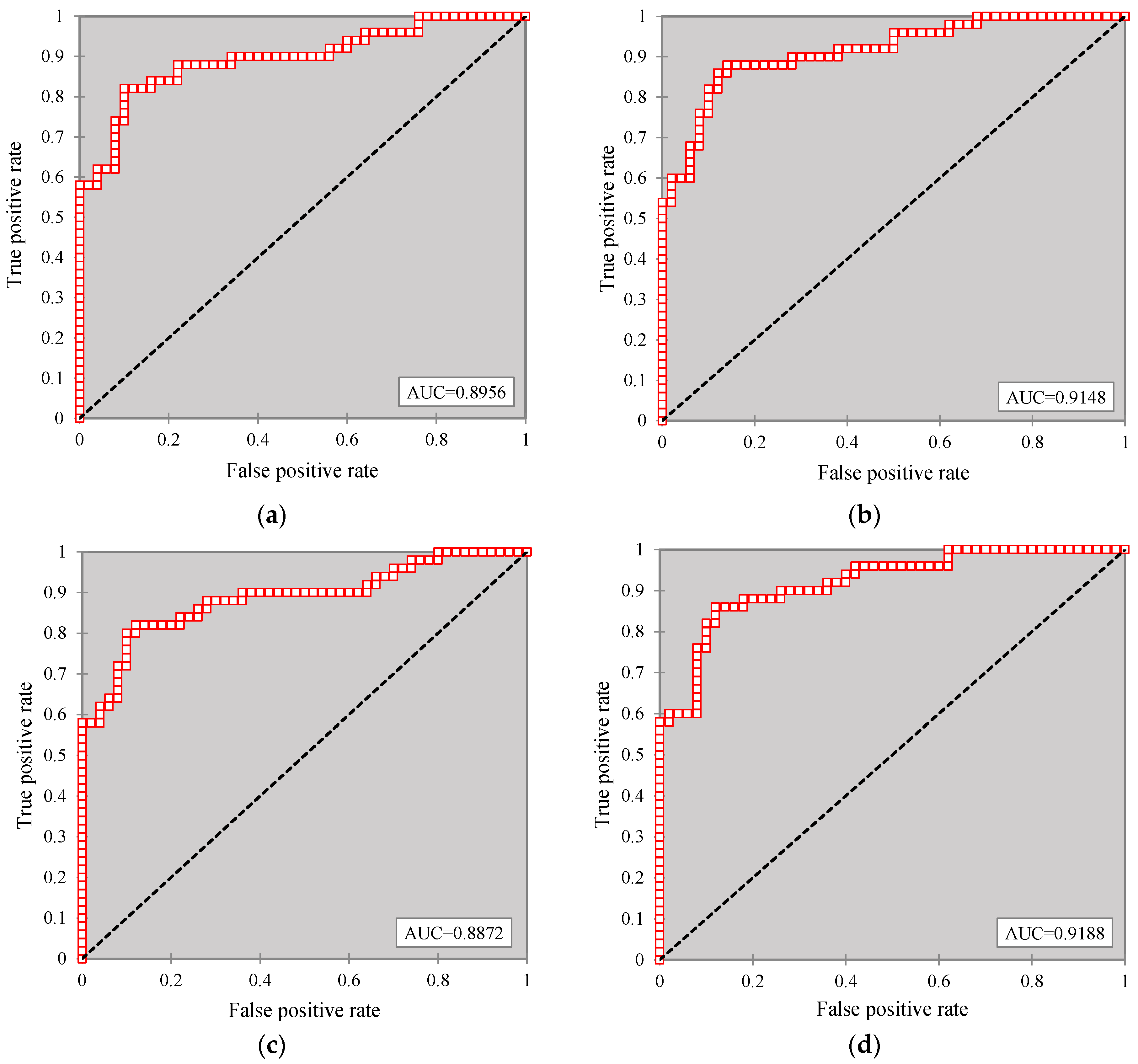
In order to assess the results of classification models generated by various kernel functions, we used the AUC to analyze the performance results. The detail grading system of AUC refers to Table 2, which is grouped into 4 categories (i.e., excellent, good, worthless and not good) corresponding to the AUC range value. The higher the AUC value, the better the classification model achieved. Figure 6 shows the result AUC values for each kernel function, i.e., polynomial, RBF, linear and sigmoid, which have the accuracy of 0.9188, 0.9148, 0.8956 and 0.8872 respectively. In terms of the accuracy’s category, the polynomial and RBF kernels are grouped into the excellent model, whereas linear and sigmoid kernels are grouped into a good model. Based on these results, it demonstrated that polynomial kernel function is chosen to be applied into our termite detection system, because this kernel has the greatest areas under the ROC curve than others. In addition, this kernel corresponds to previous evidence that it has the minimum classification error to build a hyperplane model. There is an attractive difference between the two analyses, i.e., classification error and ROC curve against the occurrence of two kernels (linear and sigmoid). Based on the result of classification error, the sigmoid is better than the linear. However, unlike the ROC curve analysis, it is clear that linear is better than sigmoid kernels. It can be explained that both approaches do not have the same concept, despite having the same aim for evaluating the classifier performance. Classification error is based on one specific cut-off, while the ROC curve tries all of the cut-offs and plots the sensitivity and specificity. However, we state that the ROC curve analysis becomes the reference for performance evaluation in current framework, since, it is widely reported that it represents the real state of a classification problem rather than the measurement of classification error [40,41].

3.4. Selected Kernel Function

The performance of the termite detection system fully depends on the kernel function. In this section, we will explain clearly how polynomial kernel works in recognizing the termite acoustic signals. First, This kernel is built using four major optimal pairs to design a hyperplane, i.e., C = 2 8 , γ = 2 1 , r = 2 2 , and d = 3.
Parameter γ has the influence on classification outcomes, because it affects the partitioning in the feature space [43]. An excessively large value for parameter γ results in over-fitting, while a disproportionately small value leads to under-fitting [44]. In addition, the parameter r, 2 2 , means that the feature space has an inhomogeneous condition consisting of all monomials, with a degree up to d [45,46]. The last, degree d controls the flexibility of the classifier result. The lowest degree (d = 1) will revert to linear kernel, which is not appropriate if the inter-feature has a non-linear relationship. According to Ben-Hur et al. [46], if d = 2, it is already flexible enough to distinguish between the two classes with a good hyperplane. If d is too large (d = 5), then it yields a similar decision boundary, with greater curvature. As can be seen in Figure 7, this is the visualization of kernel polynomial to build a reliable hyperplane. Visually, the result of hyperplane is not a linear resemblance, but it is a curve shape caused by the role of the parameter d.
The SVM classifier can manage the large features spaces, avoid overfitting by controlling the margin, and also represent using some number of samples as informative points, well-known as support vectors (SVs). The SVs give the solution to the problem in this study; if all training data sets are retrained, then this solution will not change. It can be ensured that all the characteristics in the training data set can be represented by the SVs. This is a crucial property when analyzing large data sets consisting of many uninformative patterns [47]. In common case, the number of SVs is smaller than the total training data set. In the Figure 7, the total training data are shown by circle and cross; the black circle “o” and red circle “o” describe the training dataset for infested and uninfested class respectively. However, not all the training data become SVs. For example, in this study, the numbers of support vectors employed to take a decision are 60 SVs (Figure 7), symbolized by the cross; the black cross “x” is used for SVs at infested class and red cross “x” depicts SVs for uninfested class. The true class regions are spotlighted through the symbol color (black for infested class; red for uninfested class). Similarly, the predicted class regions are visualized using a colored background that has been successfully built from the optimization process, i.e., white background for infested class and grey background for uninfested class.

4. Discussion

It should be reiterated that the current study is based on training data sets to build the classification model generated by various kernel functions and to evaluate its performance. In this study, from the four types of proposed kernels, polynomial was selected as the most effective kernel to apply into our system. The rule of this kernel is to calculate the value of f ( x i ) in Equation (7); if the result gives a positive sign (“+”), then it is classified as termite infestation, and vice versa.
This investigation is a challenging issue, because we must be able to separate the signals generated by termites and noise from the environment. Information about the presence of termites in the wood is crucial. Some of the benefits gained when this system was successfully built enable early detection, as well as help us maintain and prevent higher termite attacks on wood products. The investigation results prove scientifically that the termite acoustic signal generated by the activity of eating, foraging and head banging to the wood as an alarm signal, can be used as a parameter to detect the termites. However, it is necessary to know that we can not accurately identify the termite acoustic signal delivered by its activity. Interesting facts about the termite behavior is alarm signal for intraspecific communication; Hager and Kirchner [48] reported that the velocity of propagation of individual vibrational signals in the nest substrate was found to be about 130 m s−1.
The proposed termite detection system is a new approach that employs an artificially intelligent SVM and polynomial kernel as a strategy for recognizing termites’ acoustic signals. As pointed out previously, the SVM successfully solved this problem by providing a solution, namely the excellent classification model. As such, it can easily deal with high dimensional feature space to easily incorporate other useful features, which may improve the performance. A SVM has adjustable parameters that need to be optimized for margin maximization and error minimization. In this case, we apply the grid-search method and show satisfactory results. However, please note that there is a common method that may also be applied to search for the optimum parameter, i.e., particle swarm optimization (PSO) and genetic algorithm (GA) [43]. Hence, it remains an appealing topic for further study that can still be explored.
The success of the current system depends almost entirely on the choice of the features used to represent the object. The features (e.g., energy and entropy) proposed in this manuscript are the result of a preliminary study that has been completed by Nanda et al. [49]. Statistically, both features can indeed distinguish and characterize significantly between normal wood and wood infested by termites. We obtained these features directly in the time domain without requiring signal transformation, well-known as time domain feature. During the past decade, the time domain feature has been widely used in engineering practices and researchers due to its easy, computational simplicity and quick implementation [50,51].

5. Conclusions

Based on the experiments carried out in this study, the numbers of conclusions can be drawn. Due to termites producing acoustic signals during activities; eating, foraging, and head-banging to the wood, hence, the acoustic signal monitoring is proposed method to detect the existence of the termites. The results showed that there were significant differences in acoustic features between normal wood and wood infested by termites. Particularly, in this study, we utilized the SVM to recognize the termite acoustic signal which showed the attractive performance. Mapping input vectors into a high-dimensional feature space, the SVM introduced various kernel functions, namely linear, RBF, sigmoid and polynomial. Furthermore, the experimental results demonstrated that the SVM with polynomial kernel function achieved the best classification accuracy with AUC of 0.9188. Our system simply extracted two acoustic features derived from the time domain, e.g., energy and entropy to make a decision. Finally, in the future work, we will concentrate on: (1) the application of this technique to detect termites for different types of wood; (2) the deep investigation about SVM will also be examined, for example, the implementation of non-parallel SVM will be included into current termite detection system to provide the comprehensive result performance.

Acknowledgments

This study was financially supported by Ministry of Research, Technology and Higher Education of the Republic of Indonesia (project no. 136-SP2H-LT-DRPM-IV-2017) through the accelerated master’s program leading to doctorate research grants (PMDSU). The authors would also like to give special thanks to anonymous reviewers for their insightful comments and constructive suggestions, which greatly improved the manuscript.

Author Contributions

The initial idea of the study was comprehended by Kudang Boro Seminar and Dodi Nandika; Muhammad Achirul Nanda, Kudang Boro Seminar, Dodi Nandika, Akhiruddin Maddu did the experimental design protocol and Muhammad Achirul Nanda drafted the manuscript. All authors read and approved the final manuscript.

Conflicts of Interest

The authors declare no conflict of interest.

References

  1. Sukartana, P.; Sumarni, G.; Broadbent, S. Evaluation of chlorfluazuron in controlling the subterranean termite coptotermes curvignathus (isoptera: Rhinotermitidae) in Indonesia. J. Trop. For. Sci. 2009, 21, 13–18. [Google Scholar]
  2. Nandika, D.; Rismayadi, Y.; Diba, F. Rayap: Biologi dan Pengendaliannya, Edisi ke-2 (Termite: Biology and Its Control), 2nd ed.; Universitas Muhammadiyah Surakarta: Surakarta, Indonesia, 2015; pp. 125–139. [Google Scholar]
  3. Nandika, D.; Tjahjono, B. Initial Attack of Subterranean Termites on Acacia Crassicarpa Plantation. Available online: http://spma.org.sg/wp-content/uploads/2016/09/Day-2-1430-Dodi-Nandika.pdf (accessed on 25 December 2017).
  4. Lewis, V.R. Alternative control strategies for termites. J. Agric. Entomol. 1997, 14, 291–307. [Google Scholar]
  5. Manzoor, F. Biosensors for Termite Control. In Proceedings of the IOP: Materials Science and Engineering, Indus University, Karachi, Pakistan, 24–26 June 2013; IOP Publishing: Bristol, UK, 2013; pp. 1–3. [Google Scholar]
  6. Indrayani, Y.; Yoshimura, T.; Yanase, Y.; Fujii, Y.; Imamura, Y. Evaluation of the temperature and relative humidity preferences of the western dry-wood termite incisitermes minor (Hagen) using acoustic emission (AE) monitoring. J. Wood Sci. 2007, 53, 76–79. [Google Scholar] [CrossRef]
  7. Lewis, V.; Leighton, S.; Tabuchi, R.; Haverty, M. Seasonal and daily patterns in activity of the western drywood termite, incisitermes minor (Hagen). Insects 2011, 2, 555–563. [Google Scholar] [CrossRef] [PubMed]
  8. Lewis, V.R.; Power, A.B.; Haverty, M.I. Surface and subsurface sensor performance in acoustically detecting western drywood termites in naturally infested boards. Forest Prod. J. 2004, 54, 57–62. [Google Scholar]
  9. Mankin, R.; Osbrink, W.; Oi, F.; Anderson, J. Acoustic detection of termite infestations in urban trees. J. Econ. Entomol. 2002, 95, 981–988. [Google Scholar] [CrossRef] [PubMed]
  10. Chapman, R.F. The Insects: Structure and Function; Cambridge University Press: Cambridge, UK, 1998; p. 831. [Google Scholar]
  11. Evans, T.; Inta, R.; Lai, J.C.; Lenz, M. Foraging vibration signals attract foragers and identify food size in the drywood termite, cryptotermes secundus. Insectes Sociaux 2007, 54, 374–382. [Google Scholar] [CrossRef]
  12. Hussein, W.B.; Hussein, M.A.; Becker, T. Detection of the red palm weevil rhynchophorus ferrugineus using its bioacoustics features. Bioacoustics 2010, 19, 177–194. [Google Scholar] [CrossRef]
  13. Rach, M.M.; Gomis, H.M.; Granado, O.L.; Malumbres, M.P.; Campoy, A.M.; Martín, J.J.S. On the design of a bioacoustic sensor for the early detection of the red palm weevil. Sensors 2013, 13, 1706–1729. [Google Scholar] [CrossRef] [PubMed]
  14. Srinivas, S.; Harsha, K.S.; Sujatha, A.; Narendra, K.G. Effcient protection of palms from rpw larvae using wireless sensor networks. Int. J. Comput. Sci. 2013, 10, 192–200. [Google Scholar]
  15. Glowacz, A. Fault diagnostics of acoustic signals of loaded synchronous motor using smofs-25-expanded and selected classifiers. Teh. Vjesn. 2016, 23, 1365–1372. [Google Scholar] [CrossRef]
  16. Józwik, J. Identification and monitoring of noise sources of cnc machine tools by acoustic holography methods. Adv. Sci. Technol. Res. J. 2016, 10. [Google Scholar] [CrossRef]
  17. Glowacz, A.; Glowacz, W.; Glowacz, Z.; Kozik, J. Early fault diagnosis of bearing and stator faults of the single-phase induction motor using acoustic signals. Measurement 2018, 113, 1–9. [Google Scholar] [CrossRef]
  18. Glowacz, A.; Glowacz, Z. Diagnosis of stator faults of the single-phase induction motor using acoustic signals. Appl. Acoust. 2017, 117, 20–27. [Google Scholar] [CrossRef]
  19. Glowacz, A. Diagnostics of rotor damages of three-phase induction motors using acoustic signals and smofs-20-expanded. Arch. Acoust. 2016, 41, 507–515. [Google Scholar] [CrossRef]
  20. Green, F., III; Arango, R.A.; Boardman, C.R.; Bourne, K.J.; Hermanson, J.C.; Munson, R.A. Remote Sensing for Detection of Termite Infestations—Proof of Concept. In Proceedings of the the International Research Group on Wood Protection, Viña del Mar, Chile, 10–14 May 2015; pp. 1–10. [Google Scholar]
  21. Zhang, Y.; Wu, L. Classification of fruits using computer vision and a multiclass support vector machine. Sensors 2012, 12, 12489–12505. [Google Scholar] [CrossRef] [PubMed]
  22. SNI (Standar Nasional Indonesia). Wood and Wood Products Resistance Test to Wood Destroying Organism (SNI 01.7207-2006); Indonesian National Standard Bureau: Jakarta, Indonesia, 2006. [Google Scholar]
  23. Ciptohadijoyo, S.; Litananda, W.; Rivai, M.; Purnomo, M. Electronic nose based on partition column integrated with gas sensor for fruit identification and classification. Comput. Electron. Agric. 2016, 121, 429–435. [Google Scholar] [CrossRef]
  24. Giannakopoulos, T.; Pikrakis, A. Introduction to Audio Analysis: A Matlab® Approach; Academic Press: Cambridge, MA, USA, 2014; pp. 70–75. [Google Scholar]
  25. Hemmati, F.; Orfali, W.; Gadala, M.S. Roller bearing acoustic signature extraction by wavelet packet transform, applications in fault detection and size estimation. Appl. Acoust. 2016, 104, 101–118. [Google Scholar] [CrossRef]
  26. Jain, A.K.; Duin, R.P.W.; Mao, J. Statistical pattern recognition: A review. IEEE Trans. Pattern Anal. Mach. Intell. 2000, 22, 4–37. [Google Scholar] [CrossRef]
  27. Bakheet, S. An svm framework for malignant melanoma detection based on optimized hog features. Computation 2017, 5, 4. [Google Scholar] [CrossRef]
  28. Wang, S.; Li, Y.; Shao, Y.; Cattani, C.; Zhang, Y.; Du, S. Detection of dendritic spines using wavelet packet entropy and fuzzy support vector machine. CNS Neurol. Disord. Drug Targets (Former. Curr. Drug Targets-CNS Neurol. Disord.) 2017, 16, 116–121. [Google Scholar] [CrossRef] [PubMed]
  29. Yang, Z.-X.; Zhong, J.-H. A hybrid EEMD-based sampEn and SVD for acoustic signal processing and fault diagnosis. Entropy 2016, 18, 112. [Google Scholar] [CrossRef]
  30. Glowacz, A. Recognition of acoustic signals of induction motor using fft, smofs-10 and isvm. Eksploat. Niezawodn. 2015, 17. [Google Scholar] [CrossRef]
  31. Men, S.; Yan, L.; Liu, J.; Qian, H.; Luo, Q. A classification method for seed viability assessment with infrared thermography. Sensors 2017, 17, 845. [Google Scholar] [CrossRef] [PubMed]
  32. Bishop, C.M. Pattern Recognition and Machine Learning; Springer: Berlin, Germany, 2006; pp. 331–333. [Google Scholar]
  33. Wang, S.; Phillips, P.; Liu, A.; Du, S. Tea category identification using computer vision and generalized eigenvalue proximal svm. Fundam. Inform. 2017, 151, 325–339. [Google Scholar] [CrossRef]
  34. Zhang, Y.; Dong, Z.; Wang, S.; Ji, G.; Yang, J. Preclinical diagnosis of magnetic resonance (MR) brain images via discrete wavelet packet transform with tsallis entropy and generalized eigenvalue proximal support vector machine (GEPSVM). Entropy 2015, 17, 1795–1813. [Google Scholar] [CrossRef]
  35. Wilk-Kolodziejczyk, D.; Regulski, K.; Gumienny, G. Comparative analysis of the properties of the nodular cast iron with carbides and the austempered ductile iron with use of the machine learning and the support vector machine. Int. J. Adv. Manuf. Technol. 2016, 87, 1077–1093. [Google Scholar] [CrossRef]
  36. Karatzoglou, A.; Meyer, D.; Hornik, K. Support vector machines in R. J. Stat. Softw. 2005, 15, 1–28. [Google Scholar]
  37. Hsu, C.-W.; Chang, C.-C.; Lin, C.-J. A Practical Guide to Support Vector Classification; National Taiwan University: Taipei, Taiwan, 2003. [Google Scholar]
  38. Min, J.H.; Lee, Y.-C. Bankruptcy prediction using support vector machine with optimal choice of kernel function parameters. Expert Syst. Appl. 2005, 28, 603–614. [Google Scholar] [CrossRef]
  39. Park, S.H.; Goo, J.M.; Jo, C.-H. Receiver operating characteristic (ROC) curve: Practical review for radiologists. Korean J. Radiol. 2004, 5, 11–18. [Google Scholar] [CrossRef] [PubMed]
  40. Fawcett, T. An introduction to ROC analysis. Pattern Recognit. Lett. 2006, 27, 861–874. [Google Scholar] [CrossRef]
  41. Zhu, W.; Zeng, N.; Wang, N. Sensitivity, specificity, accuracy, associated confidence interval and roc analysis with practical sas implementations. In Proceedings of the NESUG: Health Care and Life Sciences, Baltimore, MD, USA, 14–17 November 2010; Volume 19. [Google Scholar]
  42. Bradley, A.P. The use of the area under the roc curve in the evaluation of machine learning algorithms. Pattern Recognit. 1997, 30, 1145–1159. [Google Scholar] [CrossRef]
  43. Lin, S.-W.; Ying, K.-C.; Chen, S.-C.; Lee, Z.-J. Particle swarm optimization for parameter determination and feature selection of support vector machines. Expert Syst. Appl. 2008, 35, 1817–1824. [Google Scholar] [CrossRef]
  44. Pardo, M.; Sberveglieri, G. Classification of electronic nose data with support vector machines. Sens. Actuators B Chem. 2005, 107, 730–737. [Google Scholar] [CrossRef]
  45. Zhang, M. Artificial Higher Order Neural Networks for Economics and Business; IGI Global: Derry Township, PA, USA, 2008. [Google Scholar]
  46. Ben-Hur, A.; Ong, C.S.; Sonnenburg, S.; Schölkopf, B.; Rätsch, G. Support vector machines and kernels for computational biology. PLoS Comput. Biol. 2008, 4, e1000173. [Google Scholar] [CrossRef] [PubMed]
  47. Hua, S.; Sun, Z. Support vector machine approach for protein subcellular localization prediction. Bioinformatics 2001, 17, 721–728. [Google Scholar] [CrossRef] [PubMed]
  48. Hager, F.A.; Kirchner, W.H. Vibrational long-distance communication in the termites Macrotermes natalensis and Odontotermes sp. J. Exp. Biol. 2013, 216, 3249–3256. [Google Scholar] [CrossRef] [PubMed]
  49. Nanda, M.A.; Seminar, K.B.; Nandika, D. Characteristics of acoustic emission for subterranean termite detection in wood. J. Keteknikan Pertan. 2017, 5. in press. [Google Scholar]
  50. Patel, K. A review on feature extraction methods. Int. J. Adv. Res. Electr. Electron. Instrum. Eng. 2016, 5, 823–827. [Google Scholar] [CrossRef]
  51. Daud, W.M.B.W.; Yahya, A.B.; Horng, C.S.; Sulaima, M.F.; Sudirman, R. Features extraction of electromyography signals in time domain on biceps brachii muscle. Int. J. Model. Optim. 2013, 3, 515. [Google Scholar] [CrossRef]
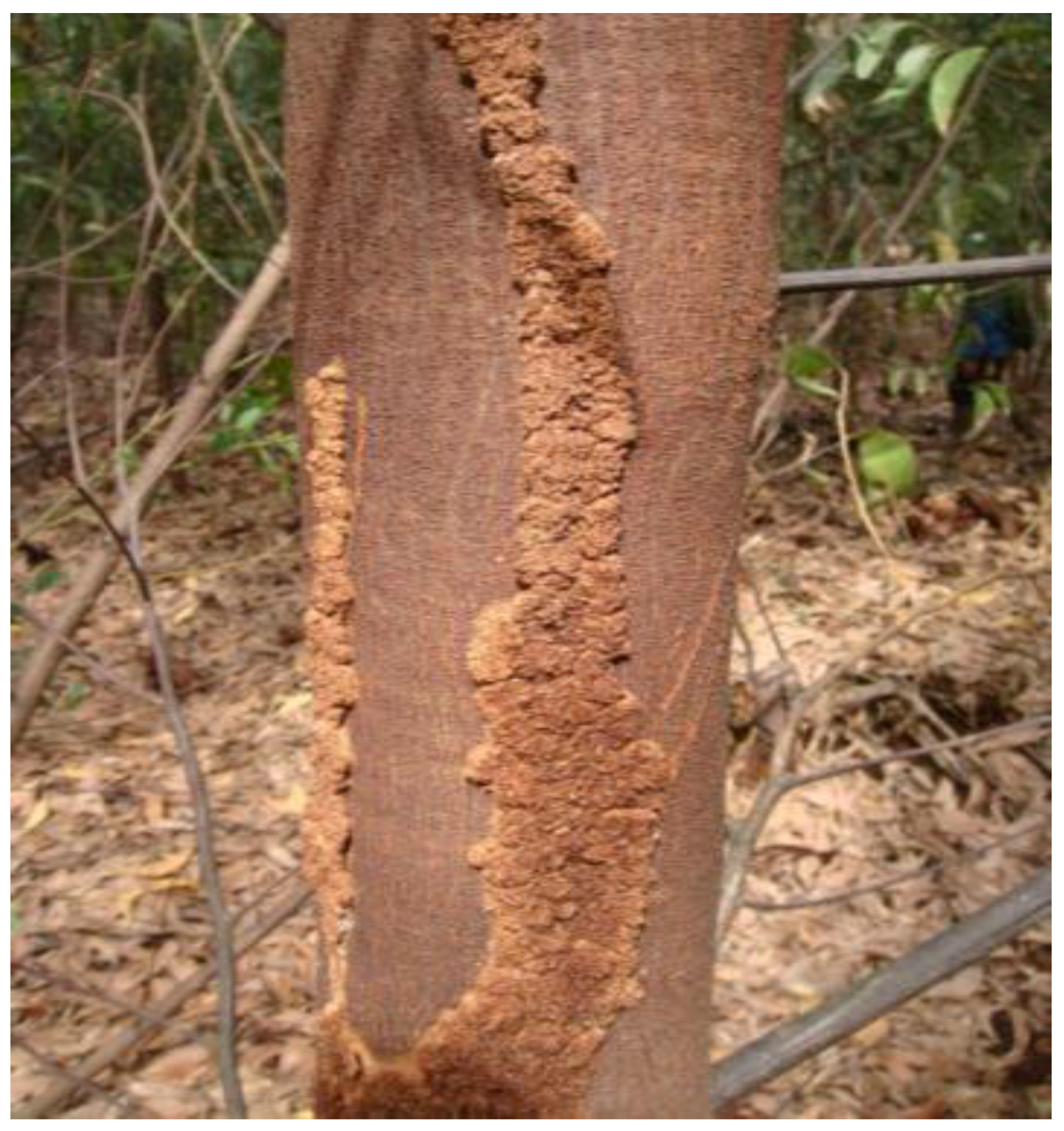
Figure 1. Initial attack of subterranean termites on Acacia crassicarpa plantation, Riau Province, Indonesia (image provided by Nandika and Tjahjono [3], used with permission).
Information 09 00005 g001
Figure 2. Schematic of the signal processing in termite detection system.
Information 09 00005 g002
Figure 3. Illustration of support vector machine (SVM) to generalize the optimal separating hyperplane in linear separable data.
Information 09 00005 g003
Figure 4. Sample of 2D plots of the feature extraction from acoustic signal acquisition.
Information 09 00005 g004
Figure 5. Grid-search on radial basis function (RBF) kernel function for finding the optimum C and γ .
Information 09 00005 g005
Figure 6. The AUC to evaluate the performance of the classifier on various kernel functions, (a) Linear; (b) RBF; (c) Sigmoid; and (d) Polynomial.
Information 09 00005 g006
Figure 7. Visualization the optimal hyperplane generated by polynomial kernel function.
Information 09 00005 g007
Table 1. Four common kernels [36].
No.Kernel FunctionFormulaOptimization Parameter
1Linear K ( x n , x i ) = ( x n , x i ) C and γ
2RBF K ( x n , x i ) = exp ( γ x n x i 2 + C ) C and γ
3Sigmoid K ( x n , x i ) = tanh ( γ ( x n , x i ) + r ) C, γ, and r
4Polynomial K ( x n , x i ) = ( γ ( x n , x i ) + r ) d C, γ, r, and d
Explanation, C: cost; γ : gamma; r: coefficient; d: degree.
Table 2. Grading system of accuracy in area under the ROC curve (AUC).
AUC RangeDescription
0.9 < AUC < 1.0Excellent
0.8 < AUC < 0.9Good
0.7 < AUC < 0.8Worthless
0.6 < AUC < 0.7Not good
Table 3. Optimal pair value in each kernel.
Kernel FunctionOptimal Pair ValueClassification Error
C γ r d
Linear2−52−10n/an/a0.17
RBF2−12−3n/an/a0.15
Sigmoid2−32−22−6n/a0.16
Polynomial2−82−12230.12