Complexity over Uncertainty in Generalized Representational Information Theory (GRIT): A Structure-Sensitive General Theory of Information

Abstract

What is information? Although researchers have used the construct of information liberally to refer to pertinent forms of domain-specific knowledge, relatively few have attempted to generalize and standardize the construct. Shannon and Weaver (1949) offered the best known attempt at a quantitative generalization in terms of the number of discriminable symbols required to communicate the state of an uncertain event. This idea, although useful, does not capture the role that structural context and complexity play in the process of understanding an event as being informative. In what follows, we discuss the limitations and futility of any generalization (and particularly, Shannon’s) that is not based on the way that agents extract patterns from their environment. More specifically, we shall argue that agent concept acquisition, and not the communication of states of uncertainty, lie at the heart of generalized information, and that the best way of characterizing information is via the relative gain or loss in concept complexity that is experienced when a set of known entities (regardless of their nature or domain of origin) changes. We show that Representational Information Theory perfectly captures this crucial aspect of information and conclude with the first generalization of RIT to continuous domains.

1. Introduction

What is information? Why is it a useful construct in science? What is the best way to measure its quantity and quality? Although these questions continue to stir profound debate in the scientific community [1,2,3,4], they have not deterred researchers from using the term “information” liberally in their work. This attitude may be explained by the common sense intuition that most humans possess about information: namely, that for an entity to be informative it must increase our knowledge about itself and, likely, about related entities. Accordingly, the greater the knowledge increase, the more informative is the entity that stimulates the increase. This common view of information, referred to here as naïve informationalism, suggests that information is partly subjective in nature. In other words, that it requires both a “knower” and an external system providing the raw material to be known. Under naïve informationalism, virtually every entity (e.g., object, feature, or event) that exists and that is perceivable may be construed as informative if it is novel and of interest to the perceiver (as known as, the “receiver”). If the entity is of tangential interest to the perceiver, it will likely not result in a significant increase in knowledge (a point that we shall revisit under Section 3 and that we refer to as information relevancy). Likewise, if the entity is familiar to the perceiver, the less likely it will be that the perceiver will experience a knowledge increase.

Naïve informationalism offers a tenable explanation as to why scientists from a wide range of disciplines, from Physics to Psychology and from Biology to Computer Science use the term “information” to refer to specific types of knowledge that characterize their particular domain of research. For example, a data analyst may be interested in the way that data may be stored in a computing device, but has no interest in the molecular interactions of a physical system. Such molecular activity is not relevant to the problems and questions of interest in the field. One could say that, to the data analyst, the entities of interest are data. Accordingly, in the field of data analysis, the terms “information” and “data” are often used interchangeably to refer to the kinds of things that a computing device is capable of storing and operating on. Similarly, for some types of physicists, the quantum states of a physical system during a certain time window comprise information. On the other hand, a behavioral psychologist may be interested on the behaviors of rats in a maze. Indeed, to a behavioral psychologist the objects of information are these behaviors. In contrast, a geneticist may find such behaviors quite tangential to his discipline. Instead, to the geneticist, knowledge about the genome of the rat is considered far more fundamental and symbol sequences (e.g., nucleotides) may be a more useful way of generalizing and thinking about the basic objects of information. All of these examples support the idea that there are as many types of information as there are domains of human knowledge [1].

In spite of these domain-specific notions of information, some scientists of the later 19th and early 20th centuries attempted to provide more general definitions of information. These attempts were often motivated, again, by development of domain specific knowledge. For example, in the field of electrical engineering, the invention of electrical technologies such as the telegraph, telephone, and radar, set the stage for a key definition of information that has influenced nearly all that have come after it. The electrical engineer Ralph Hartley proposed that information could be understood as a principle of individuation [5]. In other words, information could be operationalized in non-psychological terms, which is to say, not in terms of what increases knowledge, but as an abstract measure of the size of the message necessary to discriminate among the discriminable entities in any set. Now, this approach seemed to make perfect sense because one of the main properties possessed by all types of entities, whether sets of records (data) or sequences of nucleotides, is that they can be discriminated from other entities. However, Hartley himself succumbed to a weak form of naïve informationalism by choosing as his domain of entities strings of symbols. We say “weak” because symbols are more general and abstract constructs than many other objects studied in specialized domains, such as cells and nucleotides. Also, this was a natural choice given that Hartley’s motivation behind such characterization, by most accounts, was the transmission of messages via telegraph and other electronic means. Accordingly, in his formal framework, the amount of information transmitted could be measured in terms of the length of the message that it would take to identify any one of the elements of a set of known entities (e.g., the set of words in the English language). Henceforth, we shall refer to Hartley’s proposal as HIT (Hartley’s Information Theory).

To implement his individuation principle, Hartley proposed that the amount of information associated with any finite set of entities could be understood as a function of the size of the set. If the size of the set is a simple measure of raw information, then the “true” amount of information is given by a function that is able to specify the length of the strings or sequences of symbols (messages) necessary to discriminate (or uniquely label) all of the elements in the set. Clearly, under this criterion, the amount of information associated with a set is a much smaller number than the size of the set. Hartley proposed that the function that accomplishes this is the logarithmic function. Thus, the amount of information associated with the finite set is the logarithm to some base b of the size of X as shown in Equation (1).

(1)

For example, if we wish to compute the information content of the set S = {airplane, bus, automobile, dog}, then Equation (1) gives . This is the length of the four distinct strings of 2 symbols required to assign distinguishing labels to the 4 objects in S. As a second example, if we wish to compute the information content of the set of all the English words (about 998,000) we can set the base of the logarithm to two (for the two symbols 1 and 0) and discover that the amount of information associated with the set is approximately 20 bits. This means that it only takes a string or sequence of approximately twenty 0 and 1 symbols to discriminate any one word from all the rest of the words in the English dictionary. Note that this measure and definition of information does not concern the meaning of the words. The information content of the meaning of all the words of the English dictionary would be far greater than 20 bits, as would be the information content of any set that contains components of the original elements that are under consideration. Indeed, information as a quantity depends to a large extent on such multilevel granularity and object decomposition.

At this juncture we should clarify why the logarithmic characterization of information has achieved such an eminent status beyond simply a way of operationalizing an individuation principle. The logarithmic function embodies three desirable or ideal specifications (i.e., axioms) of an information measure. The first axiom states that information is a positive quantity and specifies the baseline quantity for information as 1 for a set of two items (a set must have at least two items for a message to carry the least amount of information other than zero). The second states that as the size of a set increases so does its amount of information. This axiom is often referred as the monotonicity axiom. Finally, the third axiom states that information as a quantity is additive in the sense that for any two finite sets X and Y, the amount of information of the Cartesian or cross product of the two sets (which consists of all the pairs of entities that can be formed by taking one entity from each set) X × Yis given by . We shall revisit these three axioms in our discussion of the probabilistic approach to information in Section 2.

The idea that information can be measured using the notion of individuation, although simple, had profound implications for subsequent measures. In fact, it was the applicability of this same notion to the probability of the value of a random variable that was the basis of Shannon’s formulation [6,7]. Although individuation is a useful construct for operationalizing and measuring information, its role in in Hartley’s measure and Shannon’s measure is indirect and higher order. In other words, the function that measures the discriminating capacity of a set (the logarithmic function) must operate on a lower level quantity that measures the “raw” amount of information of a set: Namely its cardinality or size under Hartley, and as we shall see, the probability of the value of a random variable under Shannon and Weaver (1949). One might say that this higher level measurement usually revolves around a construct that serves as the mediator or primal representation of the information. A mediator is an entity that acts as a primal encoding or representation of the information to be gained or apprehended by the observer or receiver. The nature of the mediator is dictated by the way that information is operationalized in the first place. In the case of Hartley’s measure this construct is a string or sequence of symbols—in other words, a message. Thus, we shall distinguish henceforth between mediators and carriers during our analysis, where the carriers in Hartley’s measure are sets of entities. While the carriers contain the information, the mediators make it possible for the receiver to apprehend the information conveyed by the carriers.

In the next sections we shall argue that neither way of measuring raw information reflects the true nature of information. One reason, discussed by Luce [2] and Devlin [1,4] is because the structure and meaning of the carriers of information in HIT (i.e., sets) and in Shannon–Weaver Information Theory (i.e., events) do not play a role in computing amounts of information—where by structure we mean the relationships between the elements of a set. Admittedly, attempts have been made to partially remedy this shortcoming via an extension of Shannon’s information measures to define relational information [8]. But these attempts have not yielded an elegant nor effective solution that captures the role that context or relations between components plays in shaping information as a quantity [2]. The remainder of this article will compare the classical notion and measure of information developed by Shannon and Weaver (and inspired by Hartley) to a new notion and measure of information that is structure-sensitive, meaning-sensitive, and that uses concepts and complexity as its building blocks. The theory incorporating these new ideas is known as representational information theory [9]. In the technical appendix, we discuss the formal details of RIT and, for the first time, will introduce its generalization (GRIT; generalized representational information theory) to continuous domains.

2. From Sets of Entities to Probability of Events

A second way of interpreting Hartley’s measure assumes an alternative notion of information based on the uncertainty of an event. More specifically, if we sample an element from the finite set S uniformly at random, the information revealed after we know the selection is given by the same Equation (1) above as long as we modify it slightly to include a negative sign before the logarithm function. This modification is necessary because the probability of any one item being chosen is the fraction which yields a negative quantity after its logarithm is taken. But negative information is not allowed in Hartley information theory. Again, this probabilistic interpretation is only valid when uniform random sampling is assumed. Nonetheless, it was this kind of simple insight that contributed to the generalization of information proposed by Shannon and later by Shannon and Weaver in their famous mathematical treatise on information [6,7]. Henceforth, we shall refer to their framework as SWIT (Shannon–Weaver Information Theory) and to their basic measure of information as SIM. In these two seminal papers it was suggested that by construing the carriers of information as the degrees of uncertainty of events (and not sets of objects), Hartley’s measure could be generalized to non-uniform distributions. That is, by taking the logarithm of a random variable, one could quantify information as a function of a measure of uncertainty as follows.

(2)

Shannon’s information measure appeals to our psychological intuitions about the nature of information if interpreted as meaning that the more improbable an event is, the more informative it is because its occurrence is more surprising. To explain, let x be a discrete random variable. Shannon’s measure assumes that if a highly probable value for x is detected, then the receiver has gained very little information. Accordingly, if a highly improbable value is detected, the receiver has gained a great amount of information. In other words, the amount of information received from x depends on its probability . SIM is then defined as a monotonic function (i.e., the log function to some base b, usually base 2) of the probability of x as shown in Equation (2). For example, if the event is the outcome of a single coin toss, the amount of information conveyed is the negative logarithm of the probability of the random variable x when it assumes a particular value representative of an outcome (1 for tails or 0 for heads). If the coin is equally likely to land on either side, then it has a uniform probability mass function and the amount of information transmitted by x = 1 is ½. Taking its logarithm base 2 tells us that 1 bit of information has been transmitted by knowledge that the random variable equals 1 because it requires 1 bit of information to distinguish this state of the random variable from the only other state when x is 0.

The general idea behind the basic measure proposed in SWIT is, in principle, very close to Hartley’s except that the carriers of information are now events instead of sets of entities. The primary measure of (raw) information is now the probability of a random variable and not the cardinality of a set as in Hartley’s measure. The framework attains its generality from the fact that many situations in nature can be described in terms of events and the probability distributions of their associated random variables (i.e., a measure of their uncertainty). This approach seems to be more general than Hartley’s since, as we discussed previously, the probabilistic interpretation of his measure is not consistent with non-uniform distributions [10]. In spite of this, the axiomatic recipe for Hartley’s measure, specified under the previous section, also applies to probabilities of random variables with slight modifications to the axioms. From these axioms one can prove once again that the correct function that preserves these axioms is the logarithmic function. For example, with respect to the first axiom, the logarithm of the probability of a random variable holding a particular value is a positive number as long as we add a negative sign before the logarithmic function (as in Equation (2) above).

With respect to the second axiom, the equivalent for Shannon information is that as the probability of an event increases, the amount of information associated with it decreases. This inverse relation is fully accounted for by the fact that probabilities are quantities in the real number interval: Thus, the smaller a fraction, the bigger the absolute value of its logarithm. Finally, with respect to the third axiom, information as a quantity is additive under SWIT in the sense that for any two independent events, the information gain from observing both of them is the sum of the information gain from each of them separately—more formally, —when h is the logarithmic function of the probabilities of the two events.

2.1. Criticisms of SWIT

SWIT was not intended to characterize human intuitions about the meaning of information nor was it intended to predict judgments about what humans deem informative. In fact, Shannon warned researchers of such misapplications for they fell short of the scope of his theory, which was meant to characterize communication between devices, and not provide a definitive answer to how to measure information. In spite of this, psychologists and cognitive scientists have applied Shannon’s information measure (SIM) to interpret the limits of various human cognitive capacities, such as short-term memory storage capacity [11,12] from the standpoint of the amount of information associated with particular stimuli. More recently, Deweese and Meister [13] and Butts [14] have studied the information associated with a symbol. With some minor exceptions, such links have been generally not very impressive. For example, extensive research on the connection between mean response times and the uncertainty of the stimuli to which participants responded failed to show a connection [15]. Indeed, Laming, who wrote a book on the subject many years earlier (1968) trying to establish this connection, admitted on page 642 of [15] that after extensive and unrelenting experimentation, “the idea does not work”.

In addition to these criticisms based on experimental results, the idea that uncertainty underlies informativeness does not agree with human intuitions about informativeness. Indeed, these intuitions seem to violate the inverse relation principle proposed by Barwise and Seligman (1997) which says that the rarer a piece of information the more informative it is. To begin with, the meaning and quality of any information conveyed play a role that is independent from how surprising an event may be due to its rarity or infrequency. For example, consider an observer that finds out that a bus ran through his best friend’s house the previous night without causing any bodily harm to its residents. This event may seem highly improbable and thus, very surprising to the observer. Indeed, using Shannon’s information measure, the event should be very informative. However, if instead the same observer was told that her best friend had suffered a stroke, this far more probable event would be likely perceived as more informative because of the directly impactful and vivid long chain of concepts “awakening” in the observer: for example, cancelling work to rush to the hospital, notifying relatives, spending quality time with her sick friend, etc.). In other words, the conceptual impact, context, and relevance of events determine the psychological quantity and quality of the information conveyed. This conceptual impact was summarized exquisitely by Dretske: “The utterance ‘There is a gnu in my backyard’ does not have more meaning than ‘There is a dog in my backyard’ because the former is, statistically, less probable.... To persist in this direction would lead one to the absurd view that among competent speakers of the language gibberish has more meaning than sensible discourse because it is much less frequent” (see [16], p. 42).

To further illustrate that a measure of information grounded on uncertainty cannot account for situations grounded on context and meaning, suppose that Joe wins the lottery (a one in ten million chance). The event carries information: Namely the fact that he has won. As such, the information that it carries seems disproportionately small when compared to how highly improbable and surprising the event of winning the lottery happens to be. In contrast, consider the following alternative scenario. Joe, a bird lover, lives in a wooded area with a large bird population. Joe walks into his home and discovers a dead bird on his kitchen floor. Evidently, the bird came down the cooktop vent. Nonetheless, Joe is greatly surprised to find the dead bird. The probability of birds getting caught in kitchen vents in Joe’s neighborhood is far higher that winning the lottery and Joe knows this fact. Yet, Joe is more surprised about finding a dead bird in his kitchen than about winning the lottery. Furthermore, upon asked to compare the informativeness of the two events, Joe perceives the amount of information conveyed by the “dead bird” event as greater than that conveyed by the “winning the lottery” event.

My last example addresses the subjective nature of probability judgments. In particular, the idea that these judgments are determined by the interaction of an observer with its environment. Indeed, there is empirical evidence that shows that humans will find more likely events that they have frequently experienced and, hence, commit to memory more vividly, even though such events may be objectively highly improbable [17]. Consider the following scenario: Joe has lived all his life in a town in California where earthquakes are fairly common place. Joe decides to relocate to a Midwestern town where, unbeknown to Joe, earthquakes are extremely rare. In fact, not one has occurred in fifty years. Months after his arrival, the town experiences an earthquake. To Joe, this earthquake would not seem very surprising. Yet, to the natives it will seem very surprising. This fact does not change the very different probabilities of an earthquake occurring in each location. However, given Joe’s conception of an earthquake based on his lifetime interactions with his environment, the probability he assigns to an occurrence is far higher than it ought to be under his current circumstances.

One final (and now famous) example proposed by Tversky and Kahneman in [18] illustrates the inadequacy of the classical probability measure (and its underlying axioms) as one of the building blocks of SWIT. The conjunction fallacy is a logical fallacy that occurs when it is assumed that multiple specific conditions are more probable than a single general one. The quintessential example of this fallacy comes from [18] in the form of the following script: Linda is 31 years old, single, outspoken, and very bright. She majored in philosophy. As a student, she was deeply concerned with issues of discrimination and social justice, and also participated in anti-nuclear demonstrations. Which is more probable? (1) Linda is a bank teller or (2) Linda is a bank teller and is active in the feminist movement. 90% of those asked chose option 2. However, according to classical probability theory, the probability of two events occurring together (in “conjunction”) is always less than or equal to the probability of either one occurring alone.

The above examples, among many others, demonstrate how relevance, meaning, and context, and not uncertainty, dictate our subjective sense of what is informative. They support the proposition that degrees of uncertainty (as measured by probabilities) are not a reliable marker or a sufficiently objective benchmark to serve as a quantitative measure of subjective information. In short, degree of informativeness does not hinge strictly upon what we do not know (agent uncertainty), but on what we think we know (agent certainty). The pundits might say that our examples are oversimplifications of real world situations and that recasting the described scenarios in more precise terms one may be able to make sense of the link between surprise and uncertainty. But our point is that this kind of subjective patch-up work exposes any possible link between subjective surprise and uncertainty as too fuzzy, unreliable, dubious, and noisy to serve as a basis for a rigorous quantitative theory of general information. Consequently, SWIT offers an inadequate characterization of subjective information. As mentioned, we suspect that this shortcoming is due to the fact that: (1) The carriers of SWIT are devoid of structure (i.e., the components of events and the relationships between such components are irrelevant to the theory) and (2) the probabilistic interpretation of uncertainty depends on the properties or axioms underlying the classical probability measure.

For example, using these axioms, one can define the conditional probability of an event (i.e., the probability of event A given event B); in turn, that definition is used to characterize the independence between two events A and B as equivalent to their joint probability being equal to the product of their probabilities. However, this definition, along with the definition of mutually exclusive events (i.e., events whose probability depend on other events not occurring), is psychologically implausible. For example, humans have a propensity for associating, imagining, mixing, and retrieving simultaneously or in rapid succession even the most seemingly contradictory and disparate memories. More specifically, memories and concepts of two mutually exclusive events may not be quite exclusive, independence between mental events not likely, and dependence often confounding and frequently intractable. Ergo, the human mind does not provide the necessarily ideal conditions of well-defined sample spaces and other sub-constructs for the probability axioms to apply. Furthermore, the axioms assume that the probabilities of events are additive in nature (in fact, this is one of the key characteristics of a σ-algebra, the general structure underlaying the classical probability measure). Both assumptions are too strong for modeling subjective information where context and meaning are at the heart of what it means to be informative in human communication.

Next, we shall offer an alternative way of characterizing information that overcomes the noted limitations and that conforms to our most fundamental intuitions as to the nature of information. In addition, we shall offer empirical evidence for the latter claim. Note that the motivation behind proposing an alternative way of thinking about information is not to replace or undermine SWIT. SWIT has been and will continue to be an important way of construing information within the appropriate domains. Instead, our goal is to develop a general theory of information that: (1) is based on meaning (patterns and concepts) and complexity rather than uncertainty; (2) is structure and context sensitive; and (3) it, therefore, better accounts for human intuitions and human subjective assessments as to what makes things informative.

3. Concepts and Complexity as the Building Blocks of Information

Representational Information Theory or RIT [9] was introduced as an alternative to SWIT in psychological research. The basic idea underlying the theory is that communication between animals and the environment is mediated by concepts. By a concept we mean a sparse mental representation of a set of objects in the environment that is stored in terms of the relationships between the objects in the set. The ability to form a concept from a set of objects has been a key ability for the survival of virtually every species of animal. Without this ability, animals would not be able to classify nor identify key entities linked to their survival: For example, the identification and classification of poisonous vs. nutritious food sources would not be possible. In other words, concepts (or basic generalizations about the world) are at the heart of our ability to make sense of the world around us. In particular, if a concept has been learned well, we should be able to identify any objects as belonging or not belonging to the category from which the concept emerged (for a gentle introduction to concepts see [19]).

More importantly, concepts are the “stuff” of meaning: Which means that concepts facilitate the integration of related experiences in an economical fashion and at multiple levels. This integration in turn helps facilitate storage and retrieval of concept instances from memory. For example, consider the “chair” concept which sparsely represents the set of chairs experienced up to a given point in time in a human’s lifetime. The concept has gradually been learned by extracting from the set of all known chairs key relationships between them. These key relationships we refer to as the essence of the category or set of objects being learned. Humans extract the essence of sets of objects by detecting certain kinds of patterns inherent to the set. In fact, the goal of theories of concept learning is to determine what sorts of patterns humans are most susceptible to and use as the basis for forming concepts. Among these theories, one stands out for making particularly accurate predictions as to the way that humans extract patterns from sets of objects in the environment [20,21,22]. The theory, developed by Vigo and referred to as categorical invariance theory (CIT), predicts the classification error rates of humans with respect to a large variety of categories of objects defined over two, three, and four binary and continuous dimensions. In fact, CIT and its generalization (referred to as “generalized invariance structure theory” or GIST), make very accurate predictions with respect to the data from two large-scale experiments and from numerous historical key experiments on object classification performance as shown in [21,22].

The aforementioned experiments operationalize concept learning as the ability to classify objects accurately after a set of objects (for an example, see Figure 1) is either displayed for a certain period of time (e.g., twenty seconds) or when individual objects from a set of objects are displayed one at a time serially for a brief period of time each (e.g., 3 s). The first experimental paradigm, where all the objects are displayed first before they are displayed singly in the classification phase, does not involve corrective feedback (i.e., a prompt telling the subject whether her classification decision is correct or not). On the other hand, the second paradigm, featuring the presentation of the objects one at time from the start, involves corrective feedback. The error rates in either paradigm are recorded during the experiment by a program. These classification error rates indicate the degree of concept learning difficulty of each category structure tested in the experiment. Predicting the degree of concept learning difficulty for these structures has proven to be an immensely difficult task. In fact, no theory, until CIT and GIST, has been able to accurately predict the very robust orderings of as many category structure families (84 in total; over 5000 sets of objects ranging in size from one to fifteen). Indeed, CIT and GIST account for about 90% of the variance in the data from these experiments (see [21,22]) with the introduction of a single scaling parameter. For these reasons, CIT and GIST lie at the very heart of representational information theory.

Given the fundamental role that concepts play in our mental lives and given the empirical and theoretical evidence in support of the view that organisms represent their environment conceptually, it is surprising that little formal advancement has been made linking conceptual behavior to information. If organisms are primarily conceptual filters going about the world detecting and storing the key relational patterns of sets of objects as concepts, then the raw material of information itself must be in these sets, and, more precisely, in their subsets. Then, the components of these sets of objects (its subsets), play the role of information carriers with respect to the entire set because they represent particular aspect of the entire set from which a complete concept is formed. In other words, these subsets stand for category cues to the complete concept. On the other hand, the mediators for these sets are their corresponding concepts. For example, when we wish to communicate a fact about a chair that we are not able to point to directly, we assume that the concept chair is possessed by the receiver of the message and that there is general agreement between us and the receiver as to what are the essential qualities or properties of a chair. In other words, an organism’s conceptual system determines the meaning of category cues and meaning as the basis of information. From these meanings, individuation between entities occurs implicitly.

Figure 1. Six types of structures for sets consisting of objects defined over three dimensions (color, shape, and size). The last column consists of logical descriptions of the sets.

Figure 1. Six types of structures for sets consisting of objects defined over three dimensions (color, shape, and size). The last column consists of logical descriptions of the sets.

To recap, concepts are generalizations about the world. They encompass everything that is knowable. Categories or sets of objects, on the other hand, are the material from which concepts are formed. However, unlike the sets of entities in Hartley’s theory and in SWIT, the entities that we propose have inherent components that allow for relationships to be perceived by observers. These components are simply dimensional values. Figure 1 below illustrates six sets of objects that are related in specific ways via their dimensional values. Note that we have included a logic formula under the “concept function” (see technical appendix) column to formally describe each set of objects in terms of the three constituent dimensions of color (black is represented by x' and white by x), shape (square is represented by y' and round by y), and size (small represented by z' and large by z). Also note that although the sets of objects that we have described above only feature binary dimensions, RIT has been generalized to continuous dimensions in the technical appendix of this article: the generalization is referred to as GRIT (Generalized Representational Information Theory). The generalization is a theoretically important development for both RIT and in its own right because, for the first time, it points to a precise way of thinking of the human pattern detection process described in CIT (and on which GRIT is based) as a similarity detection process. This is accomplished by what we named the “similarity-invariance principle” described in the technical appendix. To appreciate the importance of this connection, consider that similarity has been a core construct of universal science used to understand the nature of clustering patterns and category structure. On the other hand, invariance (i.e., roughly speaking, the resistance to change of a property or part of an entity when it undergoes some specific transformation or change) has played an equally prominent role in characterizing pattern. In GIST and GRIT, these two ideas are bridged in a direct, precise, and revealing fashion that should impact the way people think about both properties, and their relationship to meaning-based theories of information.

Thus far, we have defined our information carriers as subsets of sets of dimensionally-defined objects. To explain, consider sets of attributes that any of the objects of some set can have. Then, the objects can be characterized as tuples of such attributes. Thus, classes of objects are subsets of the Cartesian product of sets of attributes. For example, if the attributes come from sets X, Y, and Z, then the classes of objects are nothing but subsets of X × Y × Z (where the symbol × is the Cartesian product relation). In turn, carriers are subsets of these classes of objects. These subsets are present everywhere we look in our environment. These subsets come in the form of items we purchase at the local store to the molecules or atoms that make up a coffee cup. As long as they can be construed in terms of a finite number of constituent dimensions, they are regarded by RIT as information carriers. Moreover, there are no limits with respect to the granularity or resolution of the compositional makeup of the objects in these subsets—indeed, the choice is entirely up to the observer. These choices may range from subatomic particles, to the planets in our solar system, to symbols that make up a string.

On the other hand, we have also defined our information mediators as concepts. The concepts live in the mental space of organisms ranging from aplasia to insects and from dolphins to humans. Some may argue that they also live in the mental spaces of intelligent robots and expert systems. Regardless, the point is that only by using concepts as mediators can information as a measurable quantity reflect human intuitions as to what is informative However, the question remains: What is information and how is it measured under this view? Recall that in SWIT the information content of the carrier (event) was measured using the classical probability measure of random variables. In contrast, in HIT, it was measured by the cardinality or size of a set of objects. In RIT, the information conveyed by the carriers (subsets of dimensionally defined sets of objects) is measured by how faithful they convey the contents of the original set. This relationship between sets of objects and their subsets revolves around the complexity of sets. More specifically, it hinges upon how the degree of difficulty (or perceived complexity) of learning the set of origin (i.e., base set) changes by excluding the particular items in its information carrying subset.

But how is perceived complexity measured? As mentioned, RIT uses CIT (and its generalization, GIST) to characterize concept learning performance. In CIT, perceived complexity (or the degree of learning difficulty of a concept) is a tradeoff between the size of a set of objects (its “raw complexity”) and how much relational pattern the set of objects is perceived to have (the details of the measure are in the technical appendix). In other words, the perceived complexity of a set of objects is directly proportional to its size and inversely proportional to its degree of perceived patternfulness or structural coherence. This notion of complexity is unlike any other notion surveyed by Feldman and Crutchfield [23] in several ways. For example, although it is deterministic in nature, it not based on the notion of the “smallest program length” as is Kolmogorov-Chaitin complexity. Neither is it based on the deterministic Boolean complexity measures discussed in [24,25] nor on the notion of structural complexity studied in field of computational complexity theory which focuses on the study of complexity classes of algorithms. Even less related is statistical complexity which characterizes complexity in terms of measures of randomness. Unlike these notions of complexity, the measure of cognitive structural complexity in CIT and GIST is a phenomenological model that describes how complicated humans perceive a concept to be. Thus, the measure is truly unique in the complexity literature: Particularly because it relies on a new notion of invariance to characterize how much pattern is perceived in a stimulus.

That this approach captures the role of meaning in information may be illustrated by using the set from the first section of this article. The set S = {airplane, bus, automobile, dog} has four elements. If we ask how much information a subset of S, say a = {airplane} conveys about S, we may say quite a bit, since an airplane is part of the concept “transportation vehicle”. However, not all of the items in S are transportation vehicles, and even those objects that are transportation vehicles vary in their meaning as one. In contrast, if we ask how much information d = {dog} conveys about the set S, the answer would be very little because dogs are not directly related to transportation vehicles (i.e., they do not relate in key aspects). The way to understand this relationship is by asking what would happen to the learnability or degree of difficulty in learning a concept from the carrier S if either of the two subsets a and d were removed from S. This would answer how much relative information each subset of S has in respect to S. Why? Because when an object(s) is removed from S making S easier to learn, the absence from S contributes to the patternfulness of S. This additional regularity or patternfulness makes the set less complex (and easier to learn). But more importantly, it tells the receiver that the subset is structurally irrelevant to S or is disruptive to the regularity of S. Imagine if we remove “dog” from S. This would make S less complex and easier to learn as a concept.

Likewise, when an object(s) is removed from S making S harder to learn, the absence from S contributes to the lack of patternfulness of S. This lesser regularity or absence of patternfulness makes the set more complex (and harder to learn). It also tells the receiver that the subset is structurally relevant to S or contributes to the regularity of S. Imagine if we remove the object “airplane” from S. This would make S more complex and harder to learn as a concept. As mentioned, it turns out that RIT uses an established measure of this degree of learning difficulty or, better yet, a measure of how structurally complex a set of objects is perceived to be (see appendix for details) that has been empirically verified in [20,21,22]. But what is the amount of information conveyed by a particular carrier (subset of the base set)? The answer is the percentage change (or rate of change) of the complexity of S whenever the carrier is removed from its base set. Note that this way of measuring representational information is dimensionless. As such, the measure makes it possible to compare the informativeness conveyed by carriers consisting of any type of objects from within any domain regardless of their degree of incompatibility.

Generally, the amount of information conveyed by any carrier set is then characterized by the percentage increase or decrease in complexity experienced by the base set when the carrier subset is removed. The greater the percentage increase in base set complexity, the higher the quality of information conveyed by the carrier set; likewise, the greater the percentage decrease in base set complexity, the lower the quality of information conveyed. The information quality of the carrier is indicated by a negative sign for a negative rate of change in complexity and a positive sign for a positive rate of change in complexity. Because humans prefer a decrease in complexity, whenever there are two objects with the same magnitude in the relative rate of change in complexity of their associated category, the one with the negative sign indicates a relative higher quality of information.

The predictions made by RIT regarding the informativeness of single object carrier subsets (with respect to the six structures of four objects shown in Figure 1) was verified empirically by both judgment experiments in [26] and eye tracking experiments in [27]. These predictions are shown in Table 1 below and explained in the technical appendix. In the judgment experiments, subjects were asked to judge the degree of informativeness of each single object carrier (aka, concept cue) with respect to displayed sets of four objects as base sets. The sets of four objects shown to each subject were sampled at random from the 90(possible instances) × 24(orders) = 2160 sets of objects corresponding to the six category structures depicted in Figure 1. RIT, without free parameters, accurately predicted the degree of informativeness assigned by the subjects (on average) to each of the four objects in each of the displayed sets. In addition, RIT fitted the data very accurately, accounting, on average, for over 95% of the variance. This result showed that RIT indeed is consistent with human psychological intuitions as to the nature of information. Indeed, upon inspection of Figure 1, the reader may note that with respect to the fourth set of objects (labeled 3[4]-IV), the second object is the single most informative about the entire set (base set). However, for the first and sixth sets (labeled respectively 3[4]-I and 3[4]-VI) each object is equally informative about the entire set.

Table 1. RIT predictions corresponding to the six sets of objects shown in Figure 1.

Category	Objects	Information
3[4]-1	{001, 011, 000, 010}	[0.20, 0.20, 0.20, 0.20]
3[4]-2	{100, 001, 011, 110}	[0.05, 0.05, 0.05, 0.05]
3[4]-3	{011, 111, 000, 001}	[−0.08, −0.31, −0.31, −0.08]
3[4]-4	{000, 001, 101, 011}	[−0.31, 0.78, −0.31, −0.31]
3[4]-5	{110, 011, 000, 001}	[−0.41, −0.22, −0.22, 0.52]
3[4]-6	{001, 010, 111, 100}	[−0.25, −0.25, −0.25, −0.25]

Table 1. RIT predictions corresponding to the six sets of objects shown in Figure 1.

Category	Objects	Information
3[4]-1	{001, 011, 000, 010}	[0.20, 0.20, 0.20, 0.20]
3[4]-2	{100, 001, 011, 110}	[0.05, 0.05, 0.05, 0.05]
3[4]-3	{011, 111, 000, 001}	[−0.08, −0.31, −0.31, −0.08]
3[4]-4	{000, 001, 101, 011}	[−0.31, 0.78, −0.31, −0.31]
3[4]-5	{110, 011, 000, 001}	[−0.41, −0.22, −0.22, 0.52]
3[4]-6	{001, 010, 111, 100}	[−0.25, −0.25, −0.25, −0.25]

In addition to providing a solution to the problem of the role of meaning in information, RIT, by its very nature, also provides a way to measure the effects of structural context on the carriers of information. Recall that carriers are carriers by virtue of the relationships between the objects of the base set. But to remove any number of objects from the base set is to change its conceptual fabric or, in other words, its meaning. This functional relationship between context and meaning gives RIT a clear advantage over SWIT and HIT, and solves Luce’s (2003) concern about SWIT not capturing the structural properties of stimuli.

4. Conclusions

To summarize, in RIT, a new general way of characterizing information is proposed that is based on five principles: (1) That humans and other agents communicate via concepts or, in other words, mental representations of categories of objects (where a category is simply a set of objects that are related in some way); (2) concepts are the mediators of information; (3) concepts are mental representations of the relationships between qualitative objects in the environment that are defined dimensionally; (4) the degree of perceived homogeneity of a category (i.e., to what extent its objects are indistinguishable) as well as its cardinality (i.e., size) determine the learnability or complexity of its associated concept; and (5) information is the rate of change of that complexity. The first three principles are frequently adopted by researchers in the field of human concept learning as in [20,21,28,29,30,31,32], while principles four and five form the basis of the theory developed by Vigo [9]. These five principles support the idea that the amount of information conveyed by a set of instances about their category of origin is the rate of change in the structural complexity of the category whenever the objects are removed from it as explained in [9].

Hence, the SWIT-based notion of measuring subjective information as a function of the degree of surprise of an event is abandoned in RIT in favor of the notion that the amount of information conveyed by any subset of a category of objects about the category is the rate of change in the perceived structural complexity of the category (or, equivalently, the rate of change in the category’s degree of concept learning difficulty) when the subset is removed. More generally, the basic idea underlying RIT is that perturbations to the fabric of perceived complexity in the environment account for what we deem informative. This idea frees information from the shackles of probability theory and from the domain specific knowledge-based notions of informativeness spawned by naïve informationalism. In addition, the information measure proposed in RIT determines not only the amount of information of any dimensionally-defined object, but also its quality. More specifically, negative information values of the measure indicate a decrease in the complexity of the category when a given object is removed, whereas positive values indicate an increase in complexity with the object’s removal from the set. Also, note that the idea of linking the change in the complexity of a category structure (when some of its elements are removed) to information content addresses the problem of determining the role that context plays on the amount of information humans attribute to each object of a category. Hence, the most informative entities in a category are those that decrease its perceived complexity (for the technical details of the theory see the technical appendix).

To further contrast these ideas to HIT and SWIT, in the introduction, we made a distinction between two components of individuation-based information measures that reveal their fundamental nature: The first component measures the amount of information present in the carrier and the second operationalizes or functionalizes this quantity in terms of a principle of individuation using a mediator. We suspect that paradigm shifts in information science emerge depending on how the carrier, the mediator, and their relationship are specified. In our approach, we have proposed reassigning the role of the carriers of information to subsets of some base set of objects that are dimensionally defined and designating concepts as the mediators of information. Furthermore, the relationship between carriers and mediators was not based on a principle of individuation, but rather on a principle of differentiation: Namely, that the percentage rate of change in the complexity of any set of objects when a subset (its carrier) is removed gives the amount of information conveyed by the removed set. Again, the quality of information is measured by the sign or the direction of the slope of such rate of change.

From an ecological point of view, this characterization of information makes sense. For too long, cognitive scientists and psychologists have been greatly influenced by the belief that the environment is full of uncertainties and that behavior (and particularly, conceptual behavior) is primarily driven by uncertainty. This widespread belief explains why psychologists have attempted to use SWIT to account for cognitive performance. But uncertainty itself is a complex concept—one that depends largely on the varying frequencies of everyday experiences as managed by our conceptual system and as acquired over the course of a lifetime. This highly subjective aspect to the concept of uncertainty has been a roadblock to any kind of truly generalized information measure. The second major problem undermining SWIT as a theory of information is the fact that it plays no attention to the relationships between the carriers. Indeed, this was the crux of Luce’s criticism. RIT, on the other hand, is based exclusively on such relationships. As such, it may be used to determine the extent to which the structural context of each carrier influences the quantity and quality of information it conveys about its base set.

In closing, we have argued in this article that in order to accurately and effectively measure the amount and quality of information conveyed by stimuli in the environment, one should abandon an uncertainty-oriented conception of information in favor of one based on context, meaning, and complexity. We have discussed the assumptions and limitations of HIT and SWIT that prevent either theory from achieving such a measure. Indeed, these limitations support the proposition that any theory of subjective information that is grounded exclusively on probability theory as a measure of uncertainty is doomed to fail for it cannot capture the role that meaning (as representation) and structure play when measuring the quantity and quality of information conveyed by a set of object-stimuli. In contrast, RIT proposes that what renders an entity informative is its ability to greatly increase or decrease the perceived complexity of the surrounding environmental stimuli as determined by the observer’s conceptual system. When compared to the defining characteristics of HIT and SWIT, RIT (and its generalization to continuous domains, GRIT) successfully challenges many of our most coveted intuitions about how information should be measured.

Technical Appendix

An Introduction to Generalized Representational Information Theory (GRIT)

In this extensive technical appendix we give a simplified introduction to RIT (based largely on material from [9,21]) and its generalization, GRIT. RIT and GRIT are based on categorical invariance theory. For the formal details of categorical invariance theory and its applications to human concept learning research see [14,15,16]. The first part of this technical appendix introduces RIT; the second part introduces an extension of RIT to continuous domains using matrices. We begin by defining some terms. By a well-defined category (aka, categorical stimulus) we shall mean a set of dimensionally definable objects in the environment, or a set of memory traces (i.e., exemplars) of such objects, that, by virtue of being defined by the same dimensions, are related in some way. Concepts, on the other hand, we shall define roughly as mental representations of these categorical stimuli. Accordingly, categorical stimuli are the raw material from which concepts are formed. Dimensionally definable stimulus objects are objects that can be characterized in terms of a fixed number of shared attributes or properties (i.e., dimensions), each ranging over a continuum or over discrete values. For example, the properties of brightness, shape, and size, as well as the more subjective attributes of satisfaction and personal worth, are all possible dimensions of the objects of some stimulus set. In addition, we shall assume that all of the dimensions associated with a specific stimulus set range over a specific and fixed number of values that combined specify a gradient (standardized in the interval) for the particular dimensions. For example, the brightness dimension may have five fixed values representing five levels of brightness in a continuum standardized from 0 to 1 (from least bright to most bright).

Six examples of categorical stimuli consisting of objects defined over the discrete binary dimensions of color, shape, and size were shown in Figure 1. Note that each of the six categorical stimuli has a certain structure, which is to say that each displays a specific relationship between its dimensional values. These structures, due to their specific binary dimensional nature, are represented by Boolean algebraic or, simply stated, logical rules (i.e., expressions consisting of disjunctions, conjunctions, and negations of variables that stand for binary dimensions). These algebraic representations of a stimulus set are referred to as concept functions. Concept functions are useful in spelling out the logical structure of a stimulus set. For example, suppose that stands for blue, stands for red, stands for round, and stands for square, then the two-variable concept function (where “ ” denotes “or”, “ ” denotes “and”, and “ ” denotes “not- ”) defines the category which contains two objects: a red and round object and a blue and square object. Clearly, the choice of labels in the expression is arbitrary. Hence, there are many Boolean expressions that define the same category structure [33,34]. In this paper, concept functions will be represented by capital letters of the English alphabet (e.g., F, G, H), while the sets that such functions define in extension will be denoted by a set bracket symbol of their corresponding function symbols. For example, if F is a Boolean function in disjunctive normal form (DNF), is the category that it defines it. A DNF is a Boolean formula consisting of sums of products that are a verbatim object per object description of the category of objects (just as the example given above).

Before defining the representational information measure, we shall first define the notion of a representation (or “representative”) of a well-defined category. A representation of a well-defined category S is any subset of S. The power set is the set of all such representations. Since there are elements in , then there are possible representations of S ( stands for cardinality or size of the set S). Some representations capture the structural (i.e., relational) “essence” or nature of S better than others. In other words, some representations carry more representational information (i.e., more conceptual significance) about S than others. For example, consider a well-defined category with three objects defined over three dimensions (color, shape, and size) consisting of a small black circle, a small black square, and a large white circle. The small black circle better captures the character of the category as a whole than does the large white circle. In addition, it would seem that, (1) for any well-defined category S, all the information in S is conveyed by S itself; and that (2) the empty set carries no information about S. The aim of our measure is to measure the amount and quality of conceptual information carried by representations or representatives of the category S about S while obeying these two basic requirements and capturing the conceptual significance of S.

Categorical Invariance Theory

Categorical invariance theory is a theory of human concept learning that has been successful at accurately predicting the degree of concept learning difficulty of categories of objects (see [20,21]). The theory is based on the general idea that the way that humans learn concepts is by detecting invariance patterns in sets of objects in the environment. More specifically, the theory posits that humans detect inherent relational symmetries or invariants in sets of objects that facilitate concept formation. This type of pattern detection involves the systematic perturbing or transforming each object in a set with respect to each of its defining dimensions. To illustrate this idea, consider the category containing a square that is black and small, and a circle that is black and small, and a circle that is white and large which is described by the concept function . Let's encode the features of the objects in this category using the digits “1” and “0” so that each object may be representable by a binary string. For example, “111” stands for the first object when x = 1 = square, y = 1 = small, and z = 1 = black. Thus, the entire set can be encoded by {111, 011, 000}. If we transform this set in terms of the shape dimension by assigning the opposite shape value to each of the objects in the set, we get the perturbed set {011, 111, 100}. Now, if we compare the original set to the perturbed set, they have two objects in common with respect to the dimension of shape. Thus, two out of three objects remain the same. This proportion, referred to as the “dimensional kernel”, is a measure of the partial invariance of the category with respect to the dimension of shape. The first pane of Figure 2 illustrates this transformation. Doing this for each of the dimensions, we can form an ordered set, or vector, consisting of all the dimensional kernels (one per dimension) of the concept function or category type (see Figure 2 and the example after Equation (7)).

Figure 2. Logical manifold transformations along the dimensions of shape, color, and size for a set of objects defined over three dimensions. The fourth pane underneath the three top panes contains the pairwise symmetries revealed by the shape transformation.

Figure 2. Logical manifold transformations along the dimensions of shape, color, and size for a set of objects defined over three dimensions. The fourth pane underneath the three top panes contains the pairwise symmetries revealed by the shape transformation.

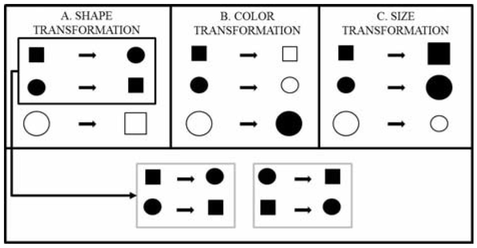
Formally, these partial invariants can be represented in terms of a vector of discrete partial derivatives of the concept function that defines the Boolean category. This is shown in Equation (5) below where stands for the logical manifold of the concept function F and where a “hat” symbol over the partial differentiation symbol indicates discrete differentiation (for a detailed and rigorous explanation, see [20,21]). Discrete partial derivatives are somewhat analogous to continuous partial derivatives in Calculus. Loosely speaking, in Calculus, the partial derivative of an n variable function is defined as how much the function value changes relative to how much the input value(s) change as seen below:

(3)

On the other hand, the discrete partial derivative, defined by the Equation below (where with ) is analogous to the continuous partial derivative except that there is no limit taken because the values of can be only 0 or 1.

(4)

The value of the derivative is ±1 if the function assignment changes when changes, and the value of the derivative is 0 if the function assignment does not change when changes. Note that the value of the derivative depends on the entire vector (abbreviated as in this note) and not just on . As an example, consider the concept function AND, denoted as (Equivalently, we could also write this function as . Because this is more readable than the vector notation, we shall continue using it in other examples.). Also, consider the particular point . At that point, the derivative of the concept function AND with respect to is 0 because the value of the concept function does not change when the stimulus changes from to . If instead we consider the point , the derivative of AND with respect to is 1 because the value of the concept function does change when the stimulus changes from to .

Accordingly, the discrete partial derivatives in Equation (5) below give the number of items that have been changed in the category in respect to a change in each of its dimensions. The double lines around the discrete partial derivatives give the proportion of objects that have not changed in the category and are defined in Equation (6) below (where is the number of objects in the category defined by the concept function F).

(5)

(6)

In the above definition (Equation (6)), stands for an object defined by D dimensional values ). The general summation symbol represents the sum of the partial derivatives evaluated at each object from the Boolean category (this is the category defined by the concept function F). The partial derivative transforms each object in respect to its i-th dimension and evaluates to 0 if, after the transformation, the object is still in (it evaluates to 1 otherwise). Thus, to compute the proportion of objects that remain in after changing the value of their -th dimension, we need to divide the sum of the partial derivatives evaluated at each object by (the number of objects in and subtract the result from 1. The absolute value symbol is placed around the partial derivative to avoid a value of negative 1 (for a detailed explanation, see [9,20,21]).

Relative degrees of total invariance across category types from different families can then be measured by taking the Euclidean distance of each structural or logical manifold (Equation (7)) from the zero logical manifold whose components are all zeros (i.e., (0,…,0)). The zero-manifold is the ideal reference point for measuring degrees of global invariance because it represents a true zero point in the subjective homogeneity scale hypothesized by the cognitive theory developed by Vigo in [20,21]. In other words, in the theory, structures with zero degree of invariance are perceived by humans as having no coherent pattern (i.e., no structural homogeneity). Thus, the overall degree of invariance of the concept function F (and of any category it defines) is given by the Equation below:

(7)

Using our example from pane one in Figure 2, we showed that the original category and the perturbed category have two elements in common (out of the three transformed elements) in respect to the shape dimension; thus, its degree of partial invariance is expressed by the ratio . Conducting a similar analysis in respect to the dimensions of color and size, its logical manifold computes to and its degree of categorical invariance is:

(8)

Note that the concept function used in our example at the beginning of Section 3 has been rewritten in an entirely equivalently form as in order to be consistent with the vector notation introduced above. Henceforth, we shall use both ways of specifying concept functions and it will be left to reader to make the appropriate translation. We do this since the non-vector notation is more intuitive and less confusing to comprehend structurally.

Invariance properties facilitate concept learning and identification. More specifically, the proposed mathematical framework reveals the pairwise symmetries that are inherent to a category structure when transformed by a change to one of its defining dimensions. One such pairwise symmetry is illustrated in the bottom pane of Figure 2. The more of these symmetries, the less the dimension is useful in determining category membership. In others words, the dimensions associated with high invariance do not help us discriminate the perturbed objects from the original objects in terms of category membership. Consequently, these particular dimensions do not carry “diagnostic” information about their associated category; however, they signal the presence of redundant information.

Structural Complexity

Using the definition of categorical invariance (Equation (7) above), we define the structural complexity of a well-defined category and its subjective structural complexity . The structural complexity of a well-defined category is directly proportional to the cardinality or size of the category (in other words, ), and indirectly proportional to a monotonically increasing function of the degree of invariance of the concept function that defines the category. This relationship is expressed formally by the parameter-free Equation (9) below where is a well-defined category. The intuition here is that the raw complexity measured by the number of items in a category is cut down or diminished by the degree of structural homogeneity or patternfullness of the category as measured by its degree of invariance.

(9)

The simplest function that meets the above criterion is the identity function. Thus, we use it as a baseline standard to define the structural complexity of a category. Moreover, since the degree of categorical invariance of the concept function F can potentially be equal to zero, we have added a 1 to to avoid division by zero in Equation (9) above. Then, the structural complexity of a category is directly proportional to its cardinality and indirectly proportional to its degree of invariance (plus one):

(10)

Although Equation (10) above is a good predictor of the perceived structural complexity of a well-defined category (as indicated by how difficult it is to apprehend it), it has been shown empirically that subjective structural complexity judgments may more accurately obey an exponentially decreasing function of its degree of invariance in [20,21,22]. Thus, we define the subjective structural complexity of a category as being directly proportional to its cardinality and indirectly proportional to the exponent of its degree of invariance.

(11)

There are parameterized variants of Equations (10) and (11) above with cognitively-motivated parameters [35]. The parameterized versions of the measures, while less parsimonious, do account for individual differences in the perception of the structural complexity of a well-defined category and, consequently, the subjective degree of difficulty experienced by human observers when acquiring concepts from their corresponding well-defined categories.

Representational Information

With the preliminary apparatus introduced, we are now in a position to introduce a measure of representational information that meets the goals set forth in the introduction to this paper. In general, a set of objects is informative about a category whenever the removal of its elements from the category increases or decreases the structural complexity of the category as a whole. That is, the amount of representational information (RI) conveyed by a representation R of a well-defined category is the rate of change of the structural complexity of . Simply stated, the representational information carried by an object or objects from a well-defined category is the percentage increase or decrease (i.e., rate of change or growth rate) in structural complexity that the category experiences whenever the object or objects are removed [36].

More specifically, let be a well-defined category defined by the concept function and let the well-defined category R be a representation of (i.e., or ). Then, if , the amount of representational information of R in respect to is determined by Equation (12) below where and stand for the number of elements in and in respectively.

(12)

Note that definitions 12 and 13 above yield negative and positive percentages. Negative percentages represent a drop in complexity. Thus, RI has two components: a magnitude and a direction (just as the value of the slope of a line indicates both magnitude and direction). For humans, the direction of RI is critical: for example, a relatively large negative value obtained from 12 and 13 above indicates that high RI is conveyed by the subset of but it characterizes the objects in the subset as highly unique or unrepresentative of those in ; while a relatively large positive value indicates that high RI is conveyed the subset of but it characterizes the objects in the subset as highly representative of those in . In the following examples, it will be shown that, intuitively, the RI values make perfect sense for representations of the same size (i.e., with the same number of objects).

Using Equation (13) above, we can compute the amount of subjective representational information associated with each representation of any category instance defined by any concept function. Take the category defined by the concept function where = square, = black, and = small used above as an example (Table 2 displays the category). To be consistent with the vector notation introduced, this concept function can also be written as: , and as before, we leave it up to the reader to make the necessary translation. As before, the objects of this category may be encoded in terms of zeros and ones, and the category may be encoded by the set {111, 011, 000} to facilitate reference to the actual objects. The amount of subjective representational information conveyed by the singleton (single element) set containing the object encoded by 111 (and defined by the rule ) in respect to the category encoded by (and defined by the concept function ) is computed as shown in 13 and 14 below:

(13)

Next, we compute the values of and and get:

(14)

Similarly, if we compute the results for the remaining two singleton (single element) representations of the set {111, 011, 000}, we get the values shown in the table of Table 2 below. 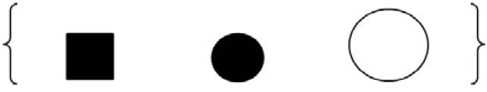These illustrate that the representation {000} is relatively less informative with respect to its category of origin {111, 011, 000} because the absence of 000 results in a 52% reduction in the structural complexity of (i.e., −0.52). Likewise, the other two singleton representations ({111} and {011}, respectively) are more informative because the absence of 111 and 000 respectively from results in a 30% increase in the structural complexity of . The reader is directed to Figure 3 below, showing a visuo-perceptual instance of the category structure, in order to confirm these results intuitively.

Table 2. Amount of Information conveyed by all the possible single element representations of .

{111}	{111, 011, 000}	{011, 000}	0.30
{011}	{111, 011, 000}	{111, 000}	0.30
{000}	{111, 011, 000}	{111, 011}	−0.52

Table 2. Amount of Information conveyed by all the possible single element representations of .

{111}	{111, 011, 000}	{011, 000}	0.30
{011}	{111, 011, 000}	{111, 000}	0.30
{000}	{111, 011, 000}	{111, 011}	−0.52

Figure 3. Category instance of concept function.

Figure 3. Category instance of concept function.

Table 3 shows the information conveyed by the single element representations of the six categories consisting with four objects defined over three dimensions (see Figure 1). Information vectors containing the amount of information conveyed by each single object representation are given in the information column. Note that each of the single element representations of category structures 3[4]-1, 3[4]-2, and 3[4]-6 respectively convey the same amount of information.

Table 3. Amount of information conveyed by all the possible single element representations of six different category types or concept functions.

Category	Objects	Information
3[4]-1	{000, 001, 100, 101}	[0.20, 0.20, 0.20, 0.20]
3[4]-2	{000, 010, 101, 111}	[0.05, 0.05, 0.05, 0.05]
3[4]-3	{101, 010, 011, 001}	[−0.31, −0.31, −0.08, −0.08]
3[4]-4	{000, 110, 011, 010}	[−0.31, −0.31, −0.31, 0.78]
3[4]-5	{011, 000, 101, 100}	[−0.41, −0.22, −0.22, 0.52]
3[4]-6	{001, 010, 100, 111}	[−0.25, −0.25, −0.25, −0.25]

Table 3. Amount of information conveyed by all the possible single element representations of six different category types or concept functions.

Category	Objects	Information
3[4]-1	{000, 001, 100, 101}	[0.20, 0.20, 0.20, 0.20]
3[4]-2	{000, 010, 101, 111}	[0.05, 0.05, 0.05, 0.05]
3[4]-3	{101, 010, 011, 001}	[−0.31, −0.31, −0.08, −0.08]
3[4]-4	{000, 110, 011, 010}	[−0.31, −0.31, −0.31, 0.78]
3[4]-5	{011, 000, 101, 100}	[−0.41, −0.22, −0.22, 0.52]
3[4]-6	{001, 010, 100, 111}	[−0.25, −0.25, −0.25, −0.25]

From Binary to Continuous Domains: The Similarity-Invariance Principle

In the above discussion, RIT has been portrayed as a theory that applies only to sets of objects or categories that are defined over binary dimensions. In order to transition to continuous dimensions with values standardized in the real number interval, all that is needed is a generalization of the structural or logical manifold (capital lambda) of a binary category so that it also applies to any continuous category. Every other aspect of the theory described above remains the same. To generalize the logical manifold operator we introduce the following equivalence between the pairwise symmetries in sets of objects (which identify pairs of invariants) and the partial similarity between the same two objects with respect to a particular dimension. Figure 4 illustrates this intuitive equivalence with respect to the shape dimension. It simply means that the relational symmetries on which categorical invariance theory is based are equivalent to pairs of objects being identical when disregarding one of their dimensions. We shall call the disregarded dimension the anchored dimension.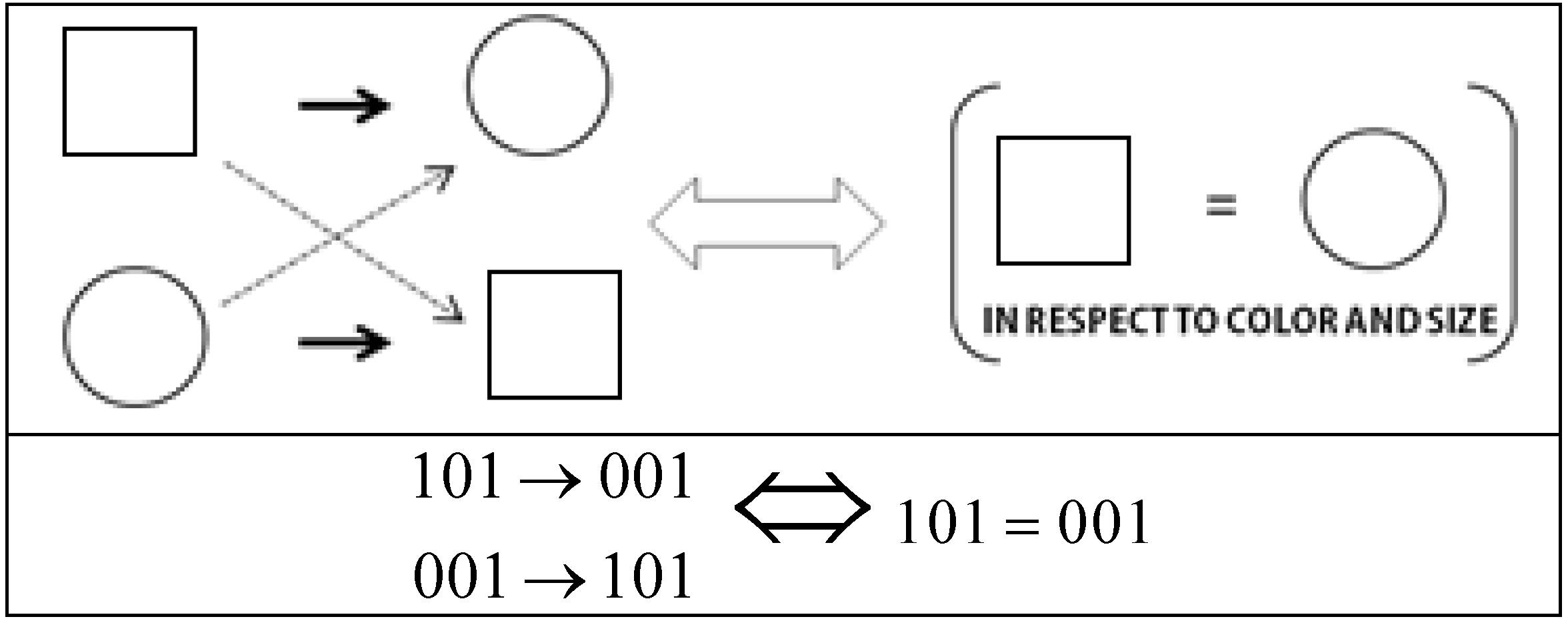

Figure 4. Equivalence of Invariance to partial similarity across two dimensions.

Figure 4. Equivalence of Invariance to partial similarity across two dimensions.

In the discussion below we shall employ the following notation:

• (1) Let be a stimulus set and stand for the cardinality (i.e., the number of elements) of X.
• (2) Let the object-stimuli in be represented by the vectors (where ).
• (3) Let the vector be the j-th D-dimensional object-stimulus in (where D is the number of dimensions of the stimulus set).
• (4) Let be the value of the i-th dimension of the j-th object-stimulus in X. We shall assume throughout our discussion that all dimensional values are real numbers greater than or equal to zero.
• (5) Let stand for the similarity of object-stimulus to object-stimulus as determined by the assumption made in multidimensional scaling theory that stimulus similarity is some monotonically decreasing function of the psychological distance between the stimuli.

We begin by describing formally the processes of dimensional binding and partial similarity assessment. To do so, we will introduce a new kind of distance operator. But first, let’s define the generalized Euclidean distance operator (aka Minkowski distance) between two object-stimuli with attention weights as:

(15)

As in the Generalized Context Model (GCM) [37], the inclusion of a parameter represents the selective attention allocated to dimension such that . We use this parameter family to represent individual differences in the process of assessing similarities between object-stimuli at this level of analysis. For the sake of simplifying our explanation and examples below, we shall disregard this parameter. Next we introduce a new kind of distance operator termed the partial psychological distance operator to model dimensional anchoring and partial similarity assessment.

(16)

Equation (16) computes the psychological distance between two stimuli ignoring their d-th dimension ( . In other words, it computes the partial psychological distance between the exemplars corresponding to the object-stimuli , by excluding dimension d in the computation of the Minkowski generalized metric. For example, if the stimulus set X consists of four object-stimuli, we represent the partial pairwise distances between the four corresponding exemplars with respect to dimension d with the following partial distances matrix:

(17)

And more generally, for any stimulus set containing p stimulus objects as:

(18)

Similarly, we can define the partial similarity between the two exemplars corresponding to the two object-stimuli—as is done in the GCM [37] and in multidimensional scaling [38,39]—as a monotonically decreasing function F of the partial distance between the two exemplars corresponding to the two object-stimuli.

(19)

In Equation (19) above, we have standardized the value in the interval using the following linear transformation where the and of a matrix are respectively its largest and smallest element, and the for any d and r.

(20)

This standardization will prove useful when we introduce the discrimination threshold parameter later in this section. As in [40], we define subjective similarity as the negative exponent of the partial distance measure and set r = 1 (i.e., we use the city block metric in our example) as shown in Equation (21) below.

(21)

In spite of using the above metric, we acknowledge the possibility that a different kind of function may be playing a similar role in the computation of partial similarities. Next we can construct the matrix of the pairwise partial psychological similarities between all four exemplars corresponding to the four object-stimuli in X as seen in Equation (22) below:

(22)

Again, as a process assumption, we have excluded reflexive or self-similarities in the diagonal of the partial distances matrix shown in Equation (22) above. However, we include symmetric comparisons since we assume that they are processed by humans when assessing the overall homogeneity of a stimulus; besides, they add to the homogeneity of the stimulus as characterized by the categorical invariance principle and the categorical invariance measure, and we wish to be consistent with both of these constructs.

Adding the values of the similarity matrix that correspond to differences within a chosen discrimination threshold for each dimension we can get the following expression which is functionally analogous to the local homogeneity operator given in Equation (6) (for any pair of objects where , , and ):

(23)

The Equation above defines the perceived degree of local homogeneity of a D-dimensional stimulus set X with respect to dimension d. is the ratio between the sum of the similarities corresponding to distances that are zero or close to zero (depending on the value of the discrimination resolution threshold) in the matrix (for a particular anchored dimension d) and the number of items in the stimulus set X. In other words, is the ratio between: (1) The sum of the similarities in the matrix (for a particular anchored dimension d) that correspond to distances in the discrimination resolution interval; and (2) the number of items in the dataset X. When the partial distances are close to zero, the points are for all intent and purpose treated as perfectly similar or identical.

For example, take a stimulus set consisting of four binary dimensions and four objects as seen in Table 4 below and represented by . Equation (24) below shows the matrix used to calculate the degree of partial homogeneity (with respect to dimension 1) of A when we let and r = 1.

Table 4. Matrix representing a stimulus set structure with four object-stimuli O1–O4 of four dimensions D1–D4.

	D1	D2	D3	D4
O1	1	1	1	0
O2	1	1	0	1
O3	1	1	0	0
O4	1	1	1	1

Table 4. Matrix representing a stimulus set structure with four object-stimuli O1–O4 of four dimensions D1–D4.

	D1	D2	D3	D4
O1	1	1	1	0
O2	1	1	0	1
O3	1	1	0	0
O4	1	1	1	1

(24)

Note that the computed matrix in Equation (24) contains 4 ones that represent four identical pairs of exemplars corresponding to four pairs of object-stimuli. Applying Equation (23) above, we get Equation (25).

(25)

Lastly, we define the generalized structural manifold by Equation (26). This construct is analogous to the global homogeneity construct defined under the binary theory, except that it applies to both binary and continuous dimensions and is equipped with a distance discrimination threshold. It measures the perceived degree of global homogeneity of any stimulus set.

(26)

We can also specify the particular degree of partial homogeneity of the structural manifold as seen in the Equation below.

(27)

We hypothesize that for every dimension the discrimination resolution threshold will be a relatively small number dependent on the discriminatory capacities of the observer. Also, the above Equation assumes that, for any d and any r, are the only partial deltas that partake in determining the partial similarity matrices. Finally, since we standardized the partial distance metric in Equation (21), then we can also say that . To simplify our discussion, in the remaining computations in this paper we shall let for all subjects and any dimension ; however, this value may also be treated as a free parameter that accounts for individual differences in classification performance. The assumption is that humans vary in their capacity to discriminate between stimuli and in their criterion for discriminating (in this paper we shall not investigate this latter option: That is, we shall not try to derive estimates for ). In either case, we assume that the primary goal of the human conceptual system is to optimize classification performance via the detection of invariants.

Table 5 below illustrates the distance and similarity matrices that represent the computation of the structural manifold of a stimulus set. The perceived degree of partial or local homogeneity is shown in the final column.

Table 5. The distance and similarity matrices associated with the computation of the local homogeneities of the stimulus set A: There are 4 structural kernels and these are listed in the last column under the perceived local homogeneity measure. Combined they form the manifold of the stimulus set A.

Dimension	Standardized						Standardized Similarity					Perceived
	Distance Matrix						Matrix					Local Homogeneity
1		1110	1101	1100	1111			1110	1101	1100	1111	0/4=0
	1110	0	1	0.5	0.5		1110	1	0.37	0.61	0.61
	1101	1	0	0.5	0.5		1101	0.37	1	0.61	0.61
	1100	0.5	0.5	0	1		1100	0.61	0.61	1	0.37
	1111	0.5	0.5	1	0		1111	0.61	0.61	0.37	1
2		1110	1101	1100	1111			1110	1101	1100	1111	0/4=0
	1110	0	1	0.5	0.5		1110	1	0.37	0.61	0.61
	1101	1	0	0.5	0.5		1101	0.37	1	0.61	0.61
	1100	0.5	0.5	0	1		1100	0.61	0.61	1	0.37
	1111	0.5	0.5	1	0		1111	0.61	0.61	0.37	1
3		1110	1101	1100	1111			1110	1101	1100	1111	4/4=1
	1110	0	1	0	1		1110	1	0.37	1	0.37
	1101	1	0	1	0		1101	0.37	1	0.37	1
	1100	0	1	0	1		1100	1	0.37	1	0.37
	1111	1	0	1	0		1111	0.37	1	0.37	1
4		1110	1101	1100	1111			1110	1101	1100	1111	4/4=1
	1110	0	1	1	0		1110	1	0.37	1	0.37
	1101	1	0	0	1		1101	0.37	1	0.37	1
	1100	1	0	0	1		1100	1	0.37	1	0.37
	1111	0	1	1	0		1111	0.37	1	0.37	1

Table 5. The distance and similarity matrices associated with the computation of the local homogeneities of the stimulus set A: There are 4 structural kernels and these are listed in the last column under the perceived local homogeneity measure. Combined they form the manifold of the stimulus set A.

Dimension	Standardized						Standardized Similarity					Perceived
	Distance Matrix						Matrix					Local Homogeneity
1		1110	1101	1100	1111			1110	1101	1100	1111	0/4=0
	1110	0	1	0.5	0.5		1110	1	0.37	0.61	0.61
	1101	1	0	0.5	0.5		1101	0.37	1	0.61	0.61
	1100	0.5	0.5	0	1		1100	0.61	0.61	1	0.37
	1111	0.5	0.5	1	0		1111	0.61	0.61	0.37	1
2		1110	1101	1100	1111			1110	1101	1100	1111	0/4=0
	1110	0	1	0.5	0.5		1110	1	0.37	0.61	0.61
	1101	1	0	0.5	0.5		1101	0.37	1	0.61	0.61
	1100	0.5	0.5	0	1		1100	0.61	0.61	1	0.37
	1111	0.5	0.5	1	0		1111	0.61	0.61	0.37	1
3		1110	1101	1100	1111			1110	1101	1100	1111	4/4=1
	1110	0	1	0	1		1110	1	0.37	1	0.37
	1101	1	0	1	0		1101	0.37	1	0.37	1
	1100	0	1	0	1		1100	1	0.37	1	0.37
	1111	1	0	1	0		1111	0.37	1	0.37	1
4		1110	1101	1100	1111			1110	1101	1100	1111	4/4=1
	1110	0	1	1	0		1110	1	0.37	1	0.37
	1101	1	0	0	1		1101	0.37	1	0.37	1
	1100	1	0	0	1		1100	1	0.37	1	0.37
	1111	0	1	1	0		1111	0.37	1	0.37	1

Combined as a vector, these four values represent all the structural information of a concept, or in other words, the ideotype of the stimulus set. The overall degree of perceived global homogeneity or invariance of a stimulus set X defined over dimensions and for any pair of objects (such that , , and ) is given by the Euclidean metric as follows:

(28)

Note the arc above the capital phi variable: It stands for the invariance measure when is able to handle objects defined over dichotomous and continuous dimensions. Equation (28) is all that is needed to generalize RIT to continuous domains (and, hence, to go convert RIT into GRIT). Thus, the final general measure is then given by the Equation below when we let be a well-defined category and let the well-defined category R be a representation of (i.e., or ). Then, if , the amount of representational information of R in respect to is determined by Equation (29) below where and stand for the number of elements in and in respectively and is the generalized perceived degree of structural complexity of a well-defined category (with normally set to 0).

(29)

References and Notes

- Devlin, K. Logic and Information; Cambridge University Press: Cambridge, UK, 1991. [Google Scholar]
- Luce, R.D. Whatever happened to information theory in psychology? Rev. Gen. Psychol. 2003, 7, 183–188. [Google Scholar] [CrossRef]
- Floridi, L. The Philosophy of Information; Oxford University Press: Oxford, UK, 2011. [Google Scholar]
- Devlin, K. Claude Shannon, 1916–2001. Focus News. Math. Assoc. Am. 2001, 21, 20–21. [Google Scholar]
- Hartley, R.V.L. Transmission of information. Bell Syst. Tech. J. 1928, 7, 535–563. [Google Scholar]
- Shannon, C.E. A mathematical theory of communication. Bell Syst. Tech. J. 1948, 27, 379–423. [Google Scholar]
- Shannon, C.E.; Weaver, W. The Mathematical Theory of Communication; University of Illinois Press: Urbana, IL, USA, 1949. [Google Scholar]
- Bishop, C.M. Pattern Recognition and Machine Learning; Springer: New York, NY, USA, 2006. [Google Scholar]
- Vigo, R. Representational information: A new general notion and measure of information. Inf. Sci. 2011, 181, 4847–4859. [Google Scholar] [CrossRef]
- Klir, G.J. Uncertainty and Information: Foundations of Generalized Information Theory; John Wiley & Sons, Inc.: Hoboken, NJ, USA, 2006. [Google Scholar]
- Miller, G.A. The magical number seven, plus or minus two: Some limits on our capacity for processing information. Psychol. Rev. 1956, 63, 81–97. [Google Scholar] [CrossRef]
- Laming, D.R.J. Information Theory of Choice-Reaction Times; Academic Press: New York, NY, USA, 1968. [Google Scholar]
- Deweese, M.R.; Meister, M. How to measure the information gained from one symbol. Network 1999, 10, 325–340. [Google Scholar] [CrossRef]
- Butts, D.A. How much information is associated with a particular stimulus? Network 2003, 14, 177–187. [Google Scholar] [CrossRef]
- Laming, D. Statistical information, uncertainty, and Bayes’ theorem: Some applications in experimental psychology. In Symbolic and Quantitative Approaches to Reasoning with Uncertainty; Benferhat, S., Besnard, P., Eds.; Springer-Verlag: Berlin, Germany, 2001; pp. 635–646. [Google Scholar]
- Dretske, F. Knowledge and the Flow of Information; MIT Press: Cambridge, MA, USA, 1981. [Google Scholar]
- Tversky, A.; Kahneman, D. Availability: A heuristic for judging frequency and probability. Cogn. Psychol. 1973, 5, 207–233. [Google Scholar] [CrossRef]
- Tversky, A.; Kahneman, D. Extension versus intuitive reasoning: The conjunction fallacy in probability judgment. Psychol. Rev. 1983, 90, 293–315. [Google Scholar] [CrossRef]
- Vigo, R. A dialogue on concepts. Think 2010, 9, 109–120. [Google Scholar] [CrossRef]
- Vigo, R. Categorical invariance and structural complexity in human concept learning. J. Math. Psychol. 2009, 53, 203–221. [Google Scholar] [CrossRef]
- Vigo, R. Towards a law of invariance in human conceptual behavior. In Proceedings of the 33rd Annual Conference of the Cognitive Science Society, Austin, TX, USA, 21 July 2011; Carlson, L., HÖlscher, C., Shipley, T., Eds.; Cognitive Science Society: Austin, TX, USA, 2011. [Google Scholar]
- Vigo, R. The gist of concepts. Cognition 2012. Submitted for publication. [Google Scholar]
- Feldman, D.; Crutchfield, J. A survey of “Complexity Measures”, Santa Fe Institute: Santa Fe, NM, USA, 11 June 1998; 1–15.
- Vigo, R. A note on the complexity of Boolean concepts. J. Math. Psychol. 2006, 50, 501–510. [Google Scholar] [CrossRef]
- Vigo, R. Modal similarity. J. Exp. Artif. Intell. 2009, 21, 181–196. [Google Scholar] [CrossRef]
- Vigo, R.; Basawaraj, B. Will the most informative object stand? Determining the impact of structural context on informativeness judgments. J. Cogn. Psychol. 2012, in press. [Google Scholar]
- Vigo, R.; Zeigler, D.; Halsey, A. Gaze and information processing during category learning: Evidence for an inverse law. Vis. Cogn. 2012. Submitted for publication. [Google Scholar]
- Bourne, L.E. Human Conceptual Behavior; Allyn and Bacon: Boston, MA, USA, 1966. [Google Scholar]
- Estes, W.K. Classification and Cognition; Oxford Psychology Series 22; Oxford University Press: Oxford, UK, 1994. [Google Scholar]
- Garner, W.R. The Processing of Information and Structure; Wiley: New York, NY, USA, 1974. [Google Scholar]
- Garner, W.R. Uncertainty and Structure as Psychological Concepts; Wiley: New York, NY, USA, 1962. [Google Scholar]
- Kruschke, J.K. ALCOVE: An exemplar-based connectionist model of category learning. Psychol. Rev. 1992, 99, 22–44. [Google Scholar] [CrossRef]
- Aiken, H.H. The staff of the Computation Laboratory at Harvard University. In Synthesis of Electronic Computing and Control Circuits; Harvard University Press: Cambridge, UK, 1951. [Google Scholar]
- Higonnet, R.A.; Grea, R.A. Logical Design of Electrical Circuits; McGraw-Hill: New York, NY, USA, 1958. [Google Scholar]
- For the readers’ convenience, the parameterized variants of Equations (10) and (11) (see main text) respectively as introduced by Vigo (2009, 2011) are as follows:
![Information 04 00001 i159]() and
and ![Information 04 00001 i160]() . The parameter
. The parameter ![Information 04 00001 i161]() in both expressions stands for a human observer’s degree of sensitivity to (i.e., extent of detection of) the invariance pattern associated with the i-th dimension (this is usually a number in the closed real interval
in both expressions stands for a human observer’s degree of sensitivity to (i.e., extent of detection of) the invariance pattern associated with the i-th dimension (this is usually a number in the closed real interval ![Information 04 00001 i009]() such that
such that ![Information 04 00001 i162]() ). k is a scaling parameter in the closed real interval
). k is a scaling parameter in the closed real interval ![Information 04 00001 i163]() (D is the number of dimensions associated with the category) that indicates the overall ability of the subject to discriminate between dimensions (a larger number indicates higher discrimination) and c is a constant parameter in the closed interval
(D is the number of dimensions associated with the category) that indicates the overall ability of the subject to discriminate between dimensions (a larger number indicates higher discrimination) and c is a constant parameter in the closed interval ![Information 04 00001 i009]() which captures possible biases displayed by observers toward invariant information (c is added to the numerator and the denominator of the ratios that make up the logical or structural manifold of the well-defined category). Finally, s is a parameter that indicates the most appropriate measure of distance as defined by the generalized Euclidean metric (i.e., the Minkowski distance measure). In our investigation, the best predictions are achieved when s = 2 (i.e., when using the Euclidean metric). Optimal estimates of these free parameters on the aggregate data provide a baseline to assess any individual differences encountered in the pattern perception stage of the concept learning process and may provide a basis for more accurate measurements of subjective representational information
which captures possible biases displayed by observers toward invariant information (c is added to the numerator and the denominator of the ratios that make up the logical or structural manifold of the well-defined category). Finally, s is a parameter that indicates the most appropriate measure of distance as defined by the generalized Euclidean metric (i.e., the Minkowski distance measure). In our investigation, the best predictions are achieved when s = 2 (i.e., when using the Euclidean metric). Optimal estimates of these free parameters on the aggregate data provide a baseline to assess any individual differences encountered in the pattern perception stage of the concept learning process and may provide a basis for more accurate measurements of subjective representational information - We could simply define the representational information of a well-defined category as the derivative of its structural complexity. We do not because our characterization of the degree of invariance of a concept function is based on a discrete counterpart to the notion of a derivative in the first place.
- Nosofsky, R.M. Choice, similarity, and the context theory of classification. J. Exp. Psychol. Learn. Mem. Cogn. 1984, 10, 104–114. [Google Scholar] [CrossRef]
- Shepard, R.N.; Romney, A.K. Multidimensional Scaling: Theory and Applications in the Behavioral Sciences; Seminar Press: New York, NY, USA, 1972; Volume I. [Google Scholar]
- Kruskal, J.B.; Wish, M. Multidimensional Scaling; Sage University Paper series on Quantitative Application in the Social Sciences 07-011; Beverly Hills and London: Beverly Hills, CA, USA, 1978. [Google Scholar]
- Shepard, R.N. Towards a universal law of generalization for psychological science. Science 1987, 237, 1317–1323. [Google Scholar]
© 2013 by the authors; licensee MDPI, Basel, Switzerland. This article is an open-access article distributed under the terms and conditions of the Creative Commons Attribution license (http://creativecommons.org/licenses/by/3.0/).
Share and Cite
Vigo, R. Complexity over Uncertainty in Generalized Representational Information Theory (GRIT): A Structure-Sensitive General Theory of Information. Information 2013, 4, 1-30. https://doi.org/10.3390/info4010001
Vigo R. Complexity over Uncertainty in Generalized Representational Information Theory (GRIT): A Structure-Sensitive General Theory of Information. Information. 2013; 4(1):1-30. https://doi.org/10.3390/info4010001
Chicago/Turabian StyleVigo, Ronaldo. 2013. "Complexity over Uncertainty in Generalized Representational Information Theory (GRIT): A Structure-Sensitive General Theory of Information" Information 4, no. 1: 1-30. https://doi.org/10.3390/info4010001
APA StyleVigo, R. (2013). Complexity over Uncertainty in Generalized Representational Information Theory (GRIT): A Structure-Sensitive General Theory of Information. Information, 4(1), 1-30. https://doi.org/10.3390/info4010001